Individual Loss Reserving Using a Gradient Boosting-Based Approach

Abstract

In this paper, we propose models for non-life loss reserving combining traditional approaches such as Mack’s or generalized linear models and gradient boosting algorithm in an individual framework. These claim-level models use information about each of the payments made for each of the claims in the portfolio, as well as characteristics of the insured. We provide an example based on a detailed dataset from a property and casualty insurance company. We contrast some traditional aggregate techniques, at the portfolio-level, with our individual-level approach and we discuss some points related to practical applications.

1. Introduction and Motivation

In its daily practice, a non-life insurance company is subject to a number of solvency constraints, e.g., ORSA guidelines in North America and Solvency II in Europe. More specifically, an actuary must predict, with the highest accuracy, future claims based on past observations. The difference between the total predicted amount and the total of all amounts already paid represents a reserve that the company must set aside. Much of the actuarial literature is devoted to the modeling, evaluation and management of this risk, see Wüthrich and Merz (2008) for an overview of existing methods.

Almost all existing models can be divided into two categories depending on the granularity of the underlying dataset: individual (or micro-level) approaches, when most information on contracts, claims, payments, etc. has been preserved, and collective (or macro-level) approaches involving some form of aggregation (often on an annual basis). The latter have been widely developed by researchers and successfully applied by practitioners for several decades. In contrast, individual approaches have been studied for decades but are currently used rarely despite the many advantages of these methods.

The idea of using an individual model for claims dates back to the early 1980s with, among others, Bühlmann et al. (1980), Hachemeister (1980) and Norberg (1986). The latter author has proposed an individual model describing the occurrence, the reporting delay and the severity of each claim separately. The idea was followed by the work of Arjas (1989), Norberg (1993, 1999), Hesselager (1994), Jewell (1989) and Haastrup and Arjas (1996). This period was characterized by very limited computing and memory resources as well as by the lack of usable data on individual claims. However, we can find some applications in Haastrup and Arjas (1996) and in some more technical documents.

Since the beginning of the 2000s, several studies have been done including, among others, the modeling of dependence using copulas Zhao and Zhou (2010), the use of generalized linear models Larsen (2007), the semi-parametric modeling of certain components Antonio and Plat (2014) and Zhao et al. (2009), the use of skew-symmetric distributions Pigeon et al. (2014), the inclusion of additional information Taylor et al. (2008), etc. Finally, some researchers have done comparisons between individual and collective approaches, often attempting to answer the question “what is the best approach?” (see Hiabu et al. (2016); Huang et al. (2015) or Charpentier and Pigeon (2016) for some examples).

Today, statistical learning techniques are widely used in the field of data analytics and may offer non-parametric solutions to claim reserving. These methods give the model more freedom and often outperform the accuracy of their parametric counterparts. However, only few approaches have been developed using micro-level information. One of them is presented in Wüthrich (2018), where the number of payments is modeled using regression trees in a discrete time framework. The occurrence of a claim payment is assumed to have a Bernoulli distribution, and the probability is then computed using a regression tree as well as all available characteristics. Other researchers, see Baudry and Robert (2017), have also developed a non-parametric approach using a machine learning algorithm known as extra-trees, an ensemble of many unpruned regression trees, for loss reserving. Finally, some researchers consider neural networks to improve classical loss reserving models (see Gabrielli et al. (2019)).

In this paper, we propose and analyze an individual model for loss reserving based on an application of a gradient boosting algorithm. Gradient boosting is a machine learning technique, that combines many “simple” models called weak learners to form a stronger predictor by optimizing some objective function. We apply an algorithm called XGBoost, see Chen and Guestrin (2016), but other machine learning techniques, such as an Extra-Trees algorithm, could also be considered.

Our strategy is to directly predict the ultimate claim amount of a file using all available information at a given time. Our approach is different from the one proposed in Wüthrich (2018) where regression trees (CART) are used to model the total number of payments per claim and/or the total amount paid per claim for each of the development periods. It is also different from the model proposed in Baudry and Robert (2017), which works recursively to build the full development of a claim, period after period.

We also present and analyze micro-level models belonging to the class of generalized linear models (GLM). Based on a detailed dataset from a property and casualty insurance company, we study some properties and we compare results obtained from various approaches. More specifically, we show that the approach combining the XGBoost algorithm and a classical collective model such as Mack’s model, has high predictive power and stability. We also propose a method for dealing with censored data and discuss the presence of dynamic covariates. We believe that the gradient boosting algorithm could be an interesting addition to the range of tools available for actuaries to evaluate the solvency of a portfolio. This case study also enriches the too short list of analyzes based on datasets from insurance companies.

In Section 2, we introduce the notation and we present the context of loss reserving from both collective and individual point of view. In Section 3, we define models based on both, generalized linear models and gradient boosting algorithm. A case study and some numerical analyses on a detailed dataset are performed in Section 4, and finally, we conclude and present some promising generalizations in Section 5.

2. Loss Reserving

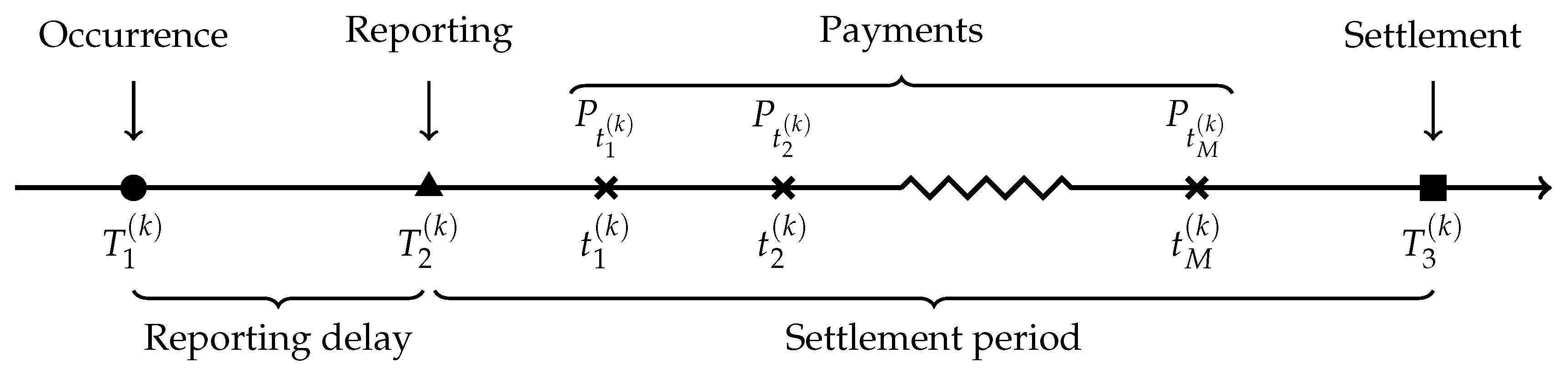
In non-life insurance, a claim always starts with an accident experienced by a policyholder that may lead to financial damages covered by an insurance contract. We call the date on which the accident happens the occurrence point ($T_1$). For some situations (bodily injury liability coverage, accident benefits, third-party responsibility liability, etc.), a reporting delay is observed between the occurrence point and the notification to the insurer at the reporting point ($T_2$). From $T_2$, the insurer could observe details about the accident, as well as some information about the insured, and record a first estimation of the final amount, called case estimate. Once the accident is reported to the insurance company, the claim is usually not settled immediately, e.g., the insurer has to investigate the case or to wait for bills or court judgments. At the reporting point $T_2$, a series of M random payments $P_{t_1},\dots ,P_{t_M}$ made respectively at times $t_1<\dots <t_M$ is therefore triggered, until the claim is closed at the settlement point ($T_3$). To simplify the presentation, all dates are expressed in number of years from an ad hoc starting point denoted by $\tau$. Finally, we need a unique index k, $k=1,\dots ,K$, to distinguish the accidents. For instance, $T_1^{(k)}$ is the occurrence date of the accident k, and $t_m^{(k)}$ is the date of the $m\mathrm{th}$ payment of this claim. Figure 1 illustrates the development of a claim.

The evaluation date $t^{*}$ is the moment on which the insurance company wants to evaluate its solvency and calculate its reserves. At this point, a claim can be classified in three categories:

• If $T_1^{(k)}<t^{*}<T_2^{(k)}$, the accident has happened but has not yet been reported to the insurer. It is therefore called an “incurred but not reported” (IBNR), claim. For one of those claims, the insurer does not have specific information about the accident, but can use policyholder and external information to estimate the reserve.
• If $T_2^{(k)}<t^{*}<T_3^{(k)}$, the accident has been reported to the insurer but is still not settled, which means the insurer expects to make additional payments to the insured. It is therefore called a “reported but not settled” (RBNS), claim. For one such claim, the historical information as well as policyholder and external information can be used to estimate the reserve.
• If $t^{*}>T_3^{(k)}$, the claim is classified as settled, or S, and the insurer does not expect to make more payments.

Finally, it is always possible for a claim to reopen after its settlement point $T_3$.

Let $C_t^{(k)}$ be a random variable representing the cumulative paid amount at date t for claim k:

$$\begin{array}{cc}\hfill C_t^{(k)}& =\left\{\begin{array}{cc}0,\hfill & t<T_2^{(k)}\hfill \\ \sum _{\{m:t_m^{(k)}\le t\}}{P}_{t_m^{(k)}},\hfill & t\ge T_2^{(k)}.\hfill \end{array}\right.\hfill \end{array}$$

At any evaluation date $T_1^{(k)}<t^{*}<T_3^{(k)}$ and for an accident k, an insurer wants to predict the cumulative paid amount at the settlement $C_{T_3}^{(k)}$, called total paid amount, by ${\widehat{C}}_{T_3}^{(k)}$ using all information available at $t^{*}$ and denoted by ${\mathcal{D}}_{t^{*}}^{(k)}$. The individual reserve for a claim evaluated at $t^{*}$ is then given by ${\widehat{R}}_{t^{*}}^{(k)}={\widehat{C}}_{T_3}^{(k)}-C_{t^{*}}^{(k)}$. For the whole portfolio, the total reserve is the aggregation of all individual reserves and is given by

$$\begin{array}{cc}\hfill {\widehat{R}}_{t^{*}}& =\sum _{k=1}^K{\widehat{R}}_{t^{*}}^{(k)}.\hfill \end{array}$$

Traditionally, insurance companies aggregate information by accident year and by development year. Claims with accident year i, $i=1,\dots ,I$, are all the claims that occurred in the $i\mathrm{th}$ year after $\tau$, which means all claims k for which $i-1<T_1^{(k)}<i$ is verified. For a claim k, a payment made in development year j, $j=1,\dots ,J=I$ is a payment made in the $j\mathrm{th}$ year after the occurrence $T_1^{(k)}$, namely a payment $P_{t_m^{(k)}}$ for which $j-1<t_m^{(k)}-T_1^{(k)}<j$. For development years $j=1,\dots ,I$, we define

$$\begin{array}{cc}\hfill Y_j^{(k)}& =\sum _{m\in {\mathcal{S}}_j^{(k)}}{P}_{t_m^{(k)}},\hfill \end{array}$$

where ${\mathcal{S}}_j^{(k)}=\{m:j-1<t_m^{(k)}-T_1^{(k)}<j\}$, as the total paid amount for claim k during year j and we define the corresponding cumulative paid amount as

$$\begin{array}{c}\hfill C_j^{(k)}=\sum _{s=1}^j{Y}_s^{(k)}.\end{array}$$

The collective group approaches every claim in the same accident year to form the aggregate incremental payment

$$\begin{array}{cc}\hfill Y_{ij}& =\sum _{k\in {\mathcal{K}}_i}{Y}_j^{(k)},i,j=1,\dots ,I,\hfill \end{array}$$

where ${\mathcal{K}}_i$ is the set of all claims with accident year i. For portfolio-level models, a prediction of the reserve at time $t^{*}$ is obtained by

$$\begin{array}{cc}\hfill {\widehat{R}}_{t^{*}}& =\sum _{i=2}^I\sum _{j=I+2-i}^I{\widehat{Y}}_{ij},\hfill \end{array}$$

(1)

where the ${\widehat{Y}}_{ij}$ are usually predicted using only the accident year and the development year.

Each cell contains a series of payments, information about the claims and some information about policyholders. These payments can also be modeled within an individual framework. Hence, a prediction of the total reserve amount is given by

$$\begin{array}{cc}\hfill {\widehat{R}}_{t^{*}}& =\underset{\mathrm{RBNS}\mathrm{reserve}}{\underbrace{\sum _{i=2}^I\sum _{j=I+2-i}^I\sum _{k\in {\mathcal{K}}_i}{\widehat{Y}}_j^{(k)}}}+\underset{\mathrm{IBNR}\mathrm{reserve}}{\underbrace{\sum _{i=2}^I\sum _{j=I+2-i}^I\sum _{k\in {\mathcal{K}}_i^{\mathrm{unobs}.}}{\widehat{Y}}_j^{(k)}}},\hfill \end{array}$$

(2)

where ${\mathcal{K}}_i^{\mathrm{unobs}.}$ is the set of IBNR claims with occurrence year i and the ${\widehat{Y}}_j^{(k)}$ can now be predicted using all available information. It should be noted that in Equations (1) and (2), we assume that all claims are paid for the earliest occurrence period ($i=1$). In this paper, we adopt this point of view and we mainly focus on estimating the RBNS reserve, which is the first part on the right-hand side of Equation (2).

3. Models for Loss Reserving

3.1. Bootstrap Mack’s Model and Generalized Linear Models for Loss Reserving

In Section 4, we compare our micro-level approach with three different types of models for loss reserving: a bootstrapped Mack’s model England and Verrall (2002), a collective GLM Wüthrich and Merz (2008) and an individual version of the latter. In order to enrich the discussion that will be done in the analysis, we briefly present in this subsection these three different approaches.

Mack’s model Mack (1993) is a distribution-free stochastic loss reserving method built for a cumulative run-off triangle. This collective model is among the most popular for loss reserving and as a result, the literature is more than substantial about it. One of the main drawbacks of this technique is that the predictive distribution of the total reserve cannot be computed directly due to the absence of a distribution assumption. In order to compare with our gradient boosting approach, we thus use a bootstrapped version of Mack’s model which allows to compute a predictive distribution. In the interest to be concise, we will not discuss more about this model, and we invite the reader to take a look at Mack (1993) and England and Verrall (2002) for more details.

In the collective GLM framework, we assume that the incremental aggregate payments $Y_{ij}$ are independent and follow a distribution falling into the exponential family with expected value given by $g\left(\mathrm{E}\left[Y_{ij}\right]\right)={\beta }_0+{\alpha }_i+{\beta }_j$, where $g()$ is the link function, ${\alpha }_i$, $i=2,3,\dots ,N$ is the accident year effect, ${\beta }_j$, $j=2,3,\dots ,N$ is the development year effect and ${\beta }_0$ is the intercept. Variance is given by $\mathrm{Var}\left[Y_{ij}\right]=\phi V\left(\mathrm{E}\left[Y_{ij}\right]\right)$, where $V()$ is the variance function and $\phi$ is the dispersion parameter (see De Jong and Heller (2008) for an introduction to GLM). The prediction for $Y_{ij}$ is then given by

$$\begin{array}{c}\hfill {\widehat{Y}}_{ij}=g^{-1}({\widehat{\beta }}_0+{\widehat{\alpha }}_i+{\widehat{\beta }}_j),\end{array}$$

where estimates of the parameters ${\widehat{\beta }}_0$, ${\{{\widehat{\alpha }}_i\}}_{i=2}^N$ and ${\{{\widehat{\beta }}_j\}}_{j=2}^N$ are usually found by maximizing likelihood. The reserve at time $t^{*}$ can thereafter be computed using Equation (1), and the predictive distribution of the total reserve can be calculated using simulations. A complete description of this model is done in Wüthrich and Merz (2008).

The individual GLM for loss reserving which we present here represents a micro-level version of the collective GLM described in the last paragraph. A major advantage of this model over the collective version comes from the use of covariates in addition to the accident and development year. Adaptations, minor or not, of our chosen approach could be studied as well, but this is not the main purpose of this paper. We assume that $Y_j^{(k)}$ follows a distribution falling into the exponential family with expected value given by $g\left(\mathrm{E}\left[Y_j^{(k)}\right]\right)={\mathit{x}}_j^{(k)}\mathit{\beta }$ and variance given by $\mathrm{Var}\left[Y_j^{(k)}\right]=\phi V\left(\mathrm{E}\left[Y_j^{(k)}\right]\right)$, where ${\mathit{x}}_j^{(k)}$ is the vector of covariates for claim k and development period j and $\mathit{\beta }$ is the usual vector of parameters. The prediction for $Y_j^{(k)}$ is obtained with

$$\begin{array}{c}\hfill {\widehat{Y}}_j^{(k)}=g^{-1}\left({\mathit{x}}_j^{(k)}\widehat{\mathit{\beta }}\right),\end{array}$$

where $\widehat{\mathit{\beta }}$ is the maximum likelihood estimator of $\mathit{\beta }$. For a claim from occurrence period i in the portfolio, the individual reserve, evaluated at $t^{*}$, is given by ${\widehat{R}}_{t^{*}}^{(k)}={\sum }_{j=I+2-i}^I{\widehat{Y}}_j^{(k)}$, and the total RBNS reserve is given by ${\widehat{R}}_{t^{*}}={\sum }_k{\widehat{R}}_{t^{*}}^{(k)}$. Some remarks should be made concerning the implementation of this model. First, the distribution of the random variable $Y_j^{(k)}$ has a mass at 0 because we did not separate occurrence and severity in our modeling. It may also be possible to consider a two-part GLM. Secondly, this model assumes that the covariates remain identical after the valuation date, which is not exactly accurate in the presence of dynamic variables such as the number of healthcare providers. We discuss this issue in more detail in the next subsection. Third, the status of a file (open or closed) is used as an explanatory variable in the model, which implicitly allows for reopening. Finally, obtaining the IBNR reserve also requires a model for the occurrence of a claim and the delay of its declaration to the insurer in addition to more assumptions about the composition of the portfolio.

3.2. Gradient Boosting for Loss Reserving

In order to train gradient boosting models, we use an algorithm called XGBoost developed by Chen and Guestrin (2016), and regression trees are chosen as weak learners. For more detail about XGBoost algorithm and regression trees, see Breiman et al. (1984); Chen and Guestrin (2016), respectively. The loss function used is the squared loss $L(y,f(\mathbf{x}))={(y-f(\mathbf{x}))}^2$ but other options such as residual deviance for gamma regression were considered without significantly altering the conclusions. A more detailed analysis of the impact of the choice of this function is deferred to a subsequent case study. Models were built using R programming language in conjunction with caret and xgboost libraries. caret is a powerful package used to train and to validate a wide range of statistical models including XGBoost algorithm.

Let us say we have a portfolio $\mathcal{S}$ on which we want to train an XGBoost model for loss reserving. This portfolio contains both, open and closed claims. At this stage, several options are available:

1.

The simplest solution is to train the model on data ${\mathcal{D}}_{\mathcal{T}}$ where only settled claims (or non-censored claims) are included. Hence, the response is known for all claims. However, this leads to a selection bias because claims that are already settled at $t^{*}$ tend to have shorter developments, and claims with shorter development tend to have lower total paid amounts. Consequently, the model is almost exclusively trained on simple claims with low training responses, which leads to underestimation of the total paid amounts for new claims. Furthermore, a significant proportion of the claims are removed from the analysis, which causes a loss of information. We will analyze this bias further in Section 4 (see model B).

2.

In Lopez et al. (2016), a different and interesting approach is proposed: in order to correct the selection bias induced by the presence of censored data, a strategy called “inverse probability of censoring weighting” (IPCW) is implemented, which involves assigning weights to observations to offset the lack of complete observations in the sample. The weights are determined using the Kaplan-Meier estimator of the censoring distribution, and a modified CART algorithm is used to make the predictions.

3.

A third approach is to develop claims that are still open at $t^{*}$ using parameters from a classical approach such as Mack’s or the GLM model. We discuss this idea in more detail in Section 4 (see model C and model D).

In order to predict total paid amount for a claim k, we use information we have about the case at evaluation date $t^{*}$, denoted by ${\mathit{x}}_{t^{*}}^{(k)}$.

Some of the covariates, such as the accident year, are static, which means their value do not change over time. These covariates are quite easy to handle because their final value is known since the reporting of the claims. However, some of the available information is expected to develop between $t^{*}$ and the closure date, for example, the claimant’s health status or the number of healthcare providers in the file. To handle those dynamic covariates, we have, at least, the following two options:

• we can assume that they are static, which can lead to a bias in the predictions obtained (see model E in Section 4); or
• we can, for each of these variables, (1) adjust a dynamic model, (2) obtain a prediction of the complete trajectory, and (3) use the algorithm conditionally to the realization of this trajectory. Moreover, there may be dependence between these variables, which would warrant a multivariate approach.

These two points will be discussed in Section 4 (see model E). The XGBoost algorithm therefore learns a prediction function ${\widehat{f}}_{XGB}$ on the adjusted dataset, depending on the selected option 1., 2. or 3. and how dynamic covariates are handled. Then, the predicted total paid amount for claim k is given by ${\widehat{C}}_{T_3}^{(k)}={\widehat{f}}_{XGB}\left({\mathit{x}}_{t^{*}}^{(k)}\right)$. Reserve for claim k is ${\widehat{R}}_{t^{*}}^{(k)}={\widehat{C}}_{T_3}^{(k)}-C_{t^{*}}^{(k)}$, and the RBNS reserve for the whole portfolio is computed with ${\widehat{R}}_{t^{*}}={\sum }_{k\in \mathcal{S}}{\widehat{R}}_{t^{*}}^{(k)}$. Gradient boosting is a non-parametric algorithm and no distribution is assumed for the response variable. Therefore, in order to compute the variance of the reserve and some risk measures, we use a non-parametric bootstrap procedure.

4. Analyses

In this section, we present an extended case study based on a detailed dataset from a property and casualty insurance company. In Section 4.1, we describe the dataset, in Section 4.2 we explain how we construct and train our models, and in Section 4.4 we present our numerical results and analyses.

4.1. Data

We analyzed a North American database consisting of $67,203$ claims occurred from 1 Januar 2004 to 31 December 2016. We therefore let $\tau$, the starting point, be 1 January 2004 meaning that all dates are expressed in number of years from this date. These claims are related to $60,075$ general liability insurance policies for private individuals. We focus only on the accident benefits coverage that provides compensation if the insured is injured or killed in an auto accident. It also includes coverage for passengers and pedestrians involved in the accident. Claims involve one ($83\%$), two ($13\%$) or $3+$ parties ($4\%$) resulting in a total of $82,520$ files in the database. Consequently, there is a possibility of dependence between some payments in the database. Nevertheless, we assume in this paper that all files are independent claims, and we postpone the analysis of this dependence. Thus, we analyze a portfolio of $82,520$ independent claims that we denote by $\mathcal{S}$. An example of the structure of the dataset is given in

Table A1. An example of the structure of the database.

Policy Number	Claim Number	Party	File Number	Date	…
P100000	C234534	1	F0000001	31 March 2004	…
P100000	C234534	1	F0000001	30 June 2004	…
P100000	C234534	1	F0000001	30 September 2004	…
…	…	…	…	…	…
P100000	C234534	2	F0000002	31 March 2004	…
P100000	C234534	2	F0000002	30 June 2004	…
P100000	C234534	2	F0000002	30 September 2004	…
…	…	…	…	…	…
P100034	C563454	1	F0000140	31 March 2004	…
P100034	C563454	1	F0000140	30 June 2004	…
P100034	C563454	1	F0000140	30 September 2004	…
…	…	…	…	…	…

Note: It can be seen that the contract P100000 generated a claim involving two people, i.e., the driver and a passenger, and generating two files. In our analysis, files F0000001 and F0000002 are considered to be independent claims. A snapshot of the available information is taken at the end of each quarter.

in Appendix A.

The data are longitudinal, and each row of the database corresponds to a snapshot of a file. For each element in $\mathcal{S}$, a snapshot is taken at the end of every quarter, and we have information from the reporting date until 31 December 2016. Therefore, a claim is represented by a maximum of 52 rows. A line is added in the database even if there is no new information, i.e., it could be possible that two consecutive lines provide precisely the same information. During the training of our models, we do not consider these replicate rows because they do not provide any relevant information for the model.

The information vector for claim k, $k=1,\dots ,82,520$ at time t is given by ${\mathcal{D}}_t^{(k)}=({\mathit{x}}_t^{(k)},C_t^{(k)})$. Therefore, the information matrix about the whole portfolio at time t is given by ${\mathcal{D}}_t^{(\mathcal{S})}={\{{\mathcal{D}}_t^{(k)}\}}_{k\in \mathcal{S}}$. Because of the discrete nature of our dataset, it contains information ${\{{\mathcal{D}}_t^{(\mathcal{S})}\}}_{\{0.25t:t\in \mathbb{N},t\le 52\}}$, where t is the number of years since $\tau$.

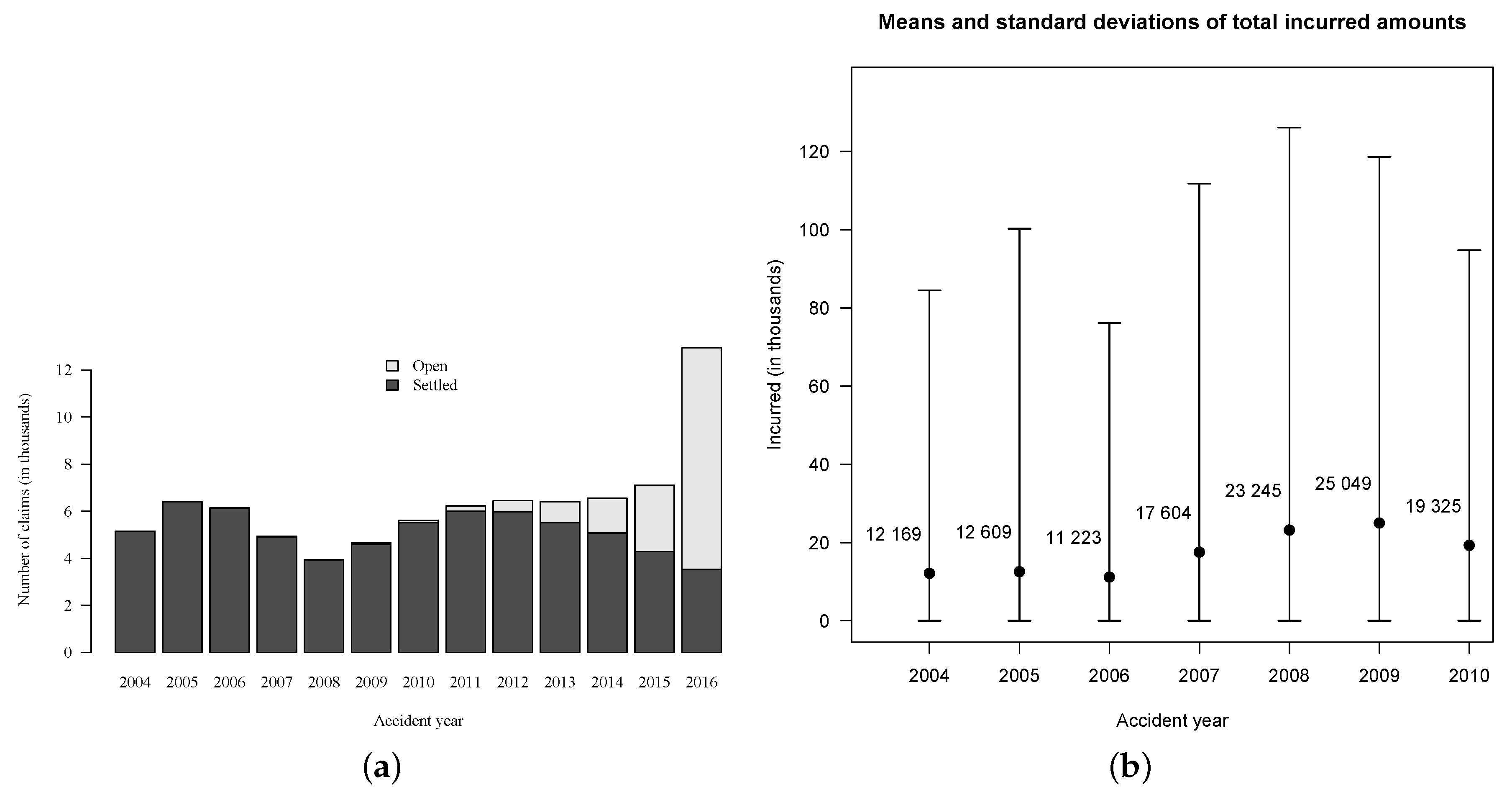
In order to validate models, we need to know how much has actually been paid for each claim. In portfolio $\mathcal{S}$, the total paid amount $C_{T_3}$ is still unknown for $19\%$ of the cases because they are related to claims that were open on 31 December 2016 (see Figure 2). To overcome this issue, we use a subset ${\mathcal{S}}_7=\{k\in \mathcal{S}:T_1^{(k)}<7\}$ of $\mathcal{S}$, i.e., we consider only accident years from 2004 to 2010 for both training and validation. This subset contains $36,286$ files related to $32,260$ claims of which $22\%$ are still open on 31 December 2010. Further, only $0.67\%$ of the files are associated with claims that are still open as of the end of 2016, so we know the exact total paid amount for $99.33\%$ of them, assuming no reopening after 2016. For the small proportion of open claims, we assume that the incurred amount set by experts is the true total paid amount. Hence, the evaluation date is set at 31 December 2010 and $t^{*}=7$. This is the date at which the reserve must be evaluated for files in ${\mathcal{S}}_7$. This implies that the models are not allowed to use information past this date for their training. Information past the evaluation date is used only for validation.

For simplicity and for computational purposes, the quarterly database is summarized to form a yearly database ${\{{\mathcal{D}}_t^{({\mathcal{S}}_7)}\}}_{t=1}^{13}$, where ${\mathcal{D}}_t^{({\mathcal{S}}_7)}={\{{\mathcal{D}}_t^{(k)}\}}_{k\in {\mathcal{S}}_7}$. We randomly sampled $70\%$ of the $36,843$ claims to form the training set of indices $\mathcal{T}\subset {\mathcal{S}}_7$, and the other $30\%$ forms the validation set of indices $\mathcal{V}\subset {\mathcal{S}}_7$, which gives the training and validation datasets ${\mathcal{D}}_{\mathcal{T}}={\{{\mathcal{D}}_t^{(\mathcal{T})}\}}_{t=1}^{13}$ and ${\mathcal{D}}_{\mathcal{V}}={\{{\mathcal{D}}_t^{(\mathcal{V})}\}}_{t=1}^{13}$.

In partnership with the insurance company, we selected 20 covariates in order to predict total paid amount for each of the claims. To make all models comparable, we use the same covariates for all claims. Some covariates are characteristics of the insured, such as age and gender, and some pertain to the claim such as the accident year, the development year, and the number of healthcare providers in the file. For privacy reasons, we cannot discuss the selected covariates further in this paper.

4.2. Training of XGBoost Models

In order to train XGBoost models, we analyze the training dataset ${\mathcal{D}}_{\mathcal{T}}={\{({\mathit{x}}_t,C_t)\}}_{t=1}^{13}$. Because some covariates are dynamic, the design matrix ${\mathit{x}}_t$ changes over time, that is to say ${\mathit{x}}_t\ne {\mathit{x}}_{t^{\prime }}$ for $t\ne t^{\prime }$. Unless otherwise stated, the models are all trained using ${\mathit{x}}_7$, which is the latest information we have about files, assuming information after $t^{*}=7$ is unknown.

Although a model using real responses is not usable in practice, it is possible to train it because we set the evaluation date to be in the past. Model A acts as a benchmark model in our case study because it is fit using $C_{T_3}$ as training responses and it is best model we can hope for. Therefore, in order to train model A, data ${\mathcal{D}}_{\mathcal{T}}^A={\{({\mathit{x}}_7^{(k)},C_{T_3}^{(k)})\}}_{k\in \mathcal{T}}$ is input into the XGBoost algorithm, which learns the prediction function ${\widehat{f}}_A$.

Model B, which is biased, is fit using $C_7$ as training responses, but only on the set of claims for which the claim is settled at time $t^{*}=7$. Hence, model B is trained using ${\mathcal{D}}_{\mathcal{T}}^B={\{({\mathit{x}}_7^{(k)},C_7^{(k)})\}}_{k\in {\mathcal{T}}_B}$, where ${\mathcal{T}}_B=\{k\in \mathcal{T}:T_3^{(k)}<7\}$, giving the prediction function ${\widehat{f}}_B$. This model allows us to measure the extent of the selection bias.

In the next models, we develop claims that are still open at $t^{*}$, i.e., we predict pseudo-responses ${\widehat{C}}_{T_3}$ using training set ${\mathcal{D}}_{\mathcal{T}}$, and these ${\widehat{C}}_{T_3}$ are subsequently used to fit the model.

In model C, claims are developed using the Mack’s model. We only develop open files at the evaluation date, i.e., we assume no reopening for settled claims. More specifically, information from data ${\{{\mathcal{D}}_t^{(\mathcal{T})}\}}_{t=1}^7$ is aggregated by accident year and by development year to form a cumulative run-off triangle. Based on this triangle, we use the bootstrap approach described in England and Verrall (2002) and involving Pearson’s residuals to generate $B=1000$ bootstrapped triangles ${\{{\mathit{C}}^{(b)}\}}_{b=1}^B$. On each of those triangles, the Mack’s model is applied to obtain vectors of development factors ${\widehat{\mathit{\lambda }}}_j={\{{\lambda }_j^{(b)}\}}_{b=1}^B$, $j=1,\dots ,6$, with

$$\begin{array}{cc}\hfill {\widehat{\lambda }}_j^{(b)}& =\frac{{\sum }_{i=1}^{7-j}{C}_{i(j+1)}^{(b)}}{{\sum }_{i=1}^{7-j}{C}_{ij}^{(b)}},b=1,\dots ,B,\hfill \end{array}$$

(3)

where $C_{i(j+1)}^{(b)}$ and $C_{ij}^{(b)}$ are from bootstrapped triangle ${\mathit{C}}^{(b)}$. From each vector ${\widehat{\mathit{\lambda }}}_j$, we compute empirical cumulative distribution function $F_j$ and we set ${\widehat{\lambda }}_j=F_j^{-1}\left({\kappa }_C\right)$, $j=1,\dots ,6$ and where ${\kappa }_C$ is a hyperparameter estimated using cross-validation. Finally, we calculate pseudo-responses ${\{{\widehat{C}}_{T_3}^{(k)}\}}_{k\in \mathcal{T}}$ using

$$\begin{array}{cc}\hfill {\widehat{C}}_{T_3}^{(k)}& ={\widehat{\lambda }}_j^c{C}_7^{(k)},\mathrm{where}{\widehat{\lambda }}_j^c=\prod _{l=j}^6{\widehat{\lambda }}_l.\hfill \end{array}$$

(4)

In model D, claims are projected using an individual quasi-Poisson GLM as described in Section 3.1 and including all 20 covariates. We discretize the amounts by rounding in order to be able to use a counting distribution even if the response variable is theoretically continuous. This approach is common in the literature associated with loss reserving and does not have a significant impact on the final results. Unlike in model C, we also develop settled claims at $t^{*}=7$. This is because in this model, the status (open or closed) of the file is used, which means the models will be able to make the difference between open and settled claims. More specifically, model D uses an individual quasi-Poisson GLM to estimate the training dependent variable. The GLM is fit on data ${\{({\mathit{x}}_t^{(\mathcal{T})},{\mathit{Y}}_t^{(\mathcal{T})})\}}_{t=1}^7$, where ${\mathit{x}}_t^{(\mathcal{T})}={\{{\mathit{x}}_t^{(k)}\}}_{k\in \mathcal{T}}$, ${\mathit{Y}}_t^{(\mathcal{T})}={\{Y_t^{(k)}\}}_{k\in \mathcal{T}}$ and $Y_t^{(k)}$ is the yearly aggregate payment at year t for claim k. A logarithm link function is used and coefficients are estimated by maximizing the Poisson log-likelihood function. Therefore, the estimation of the expected value for a new observation is given by

$$\begin{array}{c}\hfill {\widehat{\mu }}_t^{(k)}=exp\left({\mathit{x}}_t^{(k)}\widehat{\mathit{\beta }}\right),\end{array}$$

and a prediction is made according to ${\widehat{Y}}_t^{(k)}=F_{Y_t^{(k)}}^{-1}({\kappa }_D)$, which is the level ${\kappa }_D$ empirical quantile of the distribution of $Y_t^{(k)}$. This quantile can be obtained using simulation or bootstrap procedure. Finally, for the claim k, the pseudo-response is

$$\begin{array}{c}\hfill {\widehat{C}}_{T_3}^{(k)}=C_7^{(k)}+\sum _{t=8}^{13}{\widehat{Y}}_t^{(k)}.\end{array}$$

Model E is constructed in the same way as model C but it uses prospective information about the 4 dynamic stochastic covariates available in the dataset. It is analogous to model A in the sense that it is not usable in practice. However, fitting this model indicates whether an additional model that would project censored dynamic covariates would be useful. In

Table 1. Main specifications of XGBoost models.

Model	Response Variable (${\widehat{\mathit{C}}}_{{\mathit{T}}_3}$)	Covariates	Usable in Practice?
Model A	$\{C_{T_3}\}$	${\mathit{x}}_7$	No
Model B	${\{C_7^{(k)}\}}_{k\in {\mathcal{T}}_B}$, ${\mathcal{T}}_B=\{k\in \mathcal{T}:T_3^{(k)}<7\}$	${\mathit{x}}_7$	Yes
Model C	closed: $\{C_7\}$	${\mathit{x}}_7$	Yes
	open: $\{{\widehat{\lambda }}_j^c{C}_7\}$ ($\widehat{\lambda }$ from bootstrap)	${\mathit{x}}_7$
Model D	all: $\{C_7+{\sum }_{t=8}^{13}{\widehat{Y}}_t\}$ (with ${\widehat{Y}}_t=q_{{\mathit{Y}}_t}({\kappa }_D)$)	${\mathit{x}}_7$	Yes
Model E	closed: $\{C_7\}$	${\mathit{x}}_{13}$	No
	open: $\{{\widehat{\lambda }}_j^c{C}_7\}$ ($\widehat{\lambda }$ from bootstrap)	${\mathit{x}}_{13}$

Note: unless otherwise stated, we have $k\in \mathcal{T}$.

, we summarize the main specifications of the models.

4.3. Learning of Prediction Function

In Section 4.2, we showed how to train the XGBoost models having the dataset ${\mathcal{D}}_{\mathcal{T}}$. However, no details were given on how we obtain the prediction function for each model. In this section, we dive one abstraction level lower by explaining the general idea behind the algorithm. Our presentation is closely inspired by the TreeBoost algorithm developed by Friedman (2001), which is based on the same principles as XGBoost using regression trees as weak learners. The main difference between the two algorithms is the computation time: XGBoost is usually faster to train. In order to get through this, we take model A as an example. The explanation is nevertheless easily transferable to all other models since only the dataset given as input changes.

In the regression framework, a TreeBoost algorithm combines many regression trees together in order to optimize some objective function and thus learn a prediction function. The prediction function for model A takes the form of a weighted sum of regression tress

$$\begin{array}{c}\hfill {\widehat{f}}_A\left({\mathit{x}}_7^{(k)}\right)=\sum _{m=1}^M{\beta }_{m}T\left({\mathit{x}}_7^{(k)};{\mathit{\theta }}_{\mathit{m}}\right),\end{array}$$

(5)

where ${\{{\beta }_m\}}_{m=1}^M$ and ${\{{\mathit{\theta }}_m\}}_{m=1}^M$ are the weights and the vectors of parameters characterizing the regression trees, respectively. The vector of parameters associated with the $m^{\mathrm{th}}$ tree contains $J_m$ regions (or leaves) ${\{R_{jm}\}}_{j=1}^{J_m}$ as well as the corresponding prediction constants ${\{{\gamma }_{jm}\}}_{j=1}^{J_m}$, which means ${\mathit{\theta }}_m={\{R_{jm},{\gamma }_{jm}\}}_{j=1}^{J_m}$. Notice that a regression tree can be seen as a weighted sum of indicator functions:

$$\begin{array}{c}\hfill T(\mathit{x};\mathit{\theta })=\sum _{j=1}^J{\gamma }_j\mathbb{1}(\mathit{x}\in R_j).\end{array}$$

Ref. Friedman (2001) proposed to slightly modify Equation (5) in order to choose a different optimal value ${\beta }_{jm}$ for each of the tree’s regions. Consequently, each weight ${\beta }_{jm}$ can be absorbed into the prediction constant ${\gamma }_{jm}$. Assuming a constant number of regions J in each tree (which is almost always the case in practice), Equation (5) becomes

$$\begin{array}{c}\hfill {\widehat{f}}_A\left({\mathit{x}}_7^{(k)}\right)=\sum _{m=1}^M\sum _{j=1}^J{\gamma }_{jm}\mathbb{1}\left({\mathit{x}}_7^{(k)}\in R_{jm}\right).\end{array}$$

With a loss function $\mathcal{L}()$, we need to solve

$$\begin{array}{c}\hfill {\{{\beta }_m,{\mathit{\theta }}_m\}}_{m=1}^M=\underset{\{{\beta }_m^{\prime },{\mathit{\theta }}_m^{\prime }\}}{argmin}\sum _{k\in \mathcal{T}}\mathcal{L}\left(C_{T_3}^{(k)},\sum _{m=1}^M\sum _{j=1}^J{\gamma }_{jm}\mathbb{1}\left({\mathit{x}}_7^{(k)}\in R_{jm}\right)\right),\end{array}$$

which is, most of the time, too expensive computationally. The TreeBoost algorithm overcomes this issue by building the prediction function iteratively. In order to avoid overfitting, it also adds a learning rate $\nu$, $0<\nu \le 1$. The steps needed to obtain the prediction function for model A are detailed in Algorithm 1.    

algorithmAlgorithm

Algorithm 1: Obtaining ${\widehat{f}}_A$ with least square TreeBoost.

4.4. Results

From ${\{{\mathcal{D}}_t^{(\mathcal{T})}\}}_{t=1}^7$, which was the training dataset before the evaluation date, it is possible to obtain a training run-off triangle by aggregating payments by accident and by development year, presented in

Table 2. Training incremental run-off triangle (in $100,000).

Development Year	1	2	3	4	5	6	7
Accident year
2004	79	102	66	49	57	48	37
2005	83	128	84	55	52	41	·
2006	91	138	69	49	38	·	·
2007	111	155	98	61	·	·	·
2008	100	178	99	·	·	·	·
2009	137	251	·	·	·	·	·
2010	155	·	·	·	·	·	·

.

We can apply the same principle for validation dataset ${\mathcal{D}}_{\mathcal{V}}$, which yields the validation run-off triangle displayed in

Table 3. Validation incremental run-off triangle (in $100,000).

Development Year	1	2	3	4	5	6	7	$8+$
Accident year
2004	34	41	23	13	14	14	9	7
2005	37	60	36	29	45	21	20	24
2006	41	64	34	23	21	14	4	21
2007	46	67	40	37	15	18	3	13
2008	46	82	39	42	16	11	15	33
2009	54	109	62	51	31	36	11	2
2010	66	93	47	45	16	16	9	?

Note: Data used to score models are displayed in black as aggregated payments used for validation are in gray.

.

Based on the training run-off triangle, it is possible to fit many collective models, see Wüthrich and Merz (2008) for an extensive overview. Once fitted, we scored them on the validation triangle. In the validation triangle (Table 3), data used to score models are displayed in black and aggregated payments observed after the evaluation date are displayed in gray. Payments have been observed for six years after 2010, but this was not long enough for all claims to be settled. In fact, on 31 December 2016, $0.67\%$ of files were associated with claims that are still open, mostly from accident years 2009 and 2010. Therefore, amounts in column “$8+$” for accident years 2009 and 2010 in Table 3 are in fact too low. Based on available information, the observed RBNS amount was $67,619,905 (summing all gray entries), but we can reasonably think that this amount would be closer to $70,000,000 if we could observe more years. The observed IBNR amount was $3,625,983 for a total amount of $71,245,888.

Results for collective models are presented according to two approaches:

• Mack’s model, for which we present results obtained with the bootstrap approach developed by England and Verrall (2002), based on both quasi-Poisson and gamma distributions; and
• generalized linear models for which we present results obtained using a logarithmic link function and a variance function $\mathcal{V}(\mu )=\varphi {\mu }^p$ with $p=1$ (quasi-Poisson), $p=2$ (gamma), and $1<p<2$ (Tweedie).

For each model,

Table 4. Prediction results (incurred but not reported (IBNR) + reported but not settled (RBNS)) for collective approaches.

Model	Assessment	$\mathbf{E}\left[\mathbf{Res}.\right]$	$\sqrt{\mathbf{Var}\left[\mathbf{Res}.\right]}$	${\mathit{q}}_{0.95}$	${\mathit{q}}_{0.99}$
Bootstrap Mack	out-of-sample	76,795,136	7,080,826	89,086,213	95,063,184
(quasi-Poisson)	in-sample	75,019,768	8,830,631	90,242,398	97,954,554
Bootstrap Mack	out-of-sample	76,803,753	7,170,529	89,133,141	95,269,308
(Gamma)	in-sample	75,004,053	8,842,412	90,500,323	98,371,607
GLM	out-of-sample	75,706,046	2,969,877	80,655,890	82,696,002
(Quasi-Poisson)	in-sample	74,778,091	3,084,216	79,922,183	81,996,425
GLM	out-of-sample	73,518,411	2,263,714	77,276,416	78,907,812
(Gamma)	in-sample	71,277,218	3,595,958	77,343,035	80,204,504
GLM	out-of-sample	75,688,916	2,205,003	79,317,520	80,871,729
(Tweedie)	in-sample	74,706,050	2,197,659	78,260,722	79,790,056

Note: because $70\%$ of the data was used for training and $30\%$ is used for testing, we used a factor of $7/3$ to correct in-sample predictions and make them comparable with out-of-sample predictions. The observed total amount was $71,245,888.

presents the expected value of the reserve, its standard error, and the $95\%$ and the $99\%$ quantiles of the predictive distribution of the total reserve amount. As is generally the case, the choice of the distribution used to simulate the process error in the bootstrap procedure for Mack’s model has no significant impact on the results. Reasonable practices, at least in North America, generally require a reserve amount given by a high quantile ($95\%$, $99\%$ or even $99.5\%$) of the reserve’s predictive distribution. As a result, the reserve amount obtained by bootstrapping Mack’s model is too high (between $90,000,000 and $100,000,000) compared to the observed value (approximately $70,000,000). Reserve amounts obtained with generalized linear models were more reasonable (between $77,000,000 and $83,000,000), regardless of the choice of the underlying distribution. The predictive distribution for all collective models is shown in Figure 3.

In Table 4, we also present in-sample results, i.e., we used the same dataset to perform both estimation and validation. The results were very similar, which tends to indicate stability of the results obtained using these collective approaches.

Individual models were trained on the training set ${\{{\mathcal{D}}_t^{(\mathcal{T})}\}}_{t=1}^7$ and scored on the validation set ${\{{\mathcal{D}}^{(\mathcal{V})}\}}_{t=8}^{13}$. In contrast to collective approaches, individual methods used micro-covariates and, more specifically, the reporting date. This allows us to distinguish between IBNR claims and RBNS claims and, as previously mentioned, in this project we mainly focus on the modeling of the RBNS reserve. Nevertheless, in our dataset, we observe very few IBNR claims ($3,625,983) and therefore, we can reasonably compare the results obtained using both micro- and macro-level models with the observed amount ($67,619,905).

We considered the following approaches:

• individual generalized linear models (see Section 3.1), for which we present results obtained using a logarithmic link function and three variance functions: $\mathcal{V}(\mu )=\mu$ (Poisson) and $\mathcal{V}(\mu )=\varphi {\mu }^p$ with $p=1$ (quasi-Poisson) and $\mathcal{V}(\mu )=\varphi {\mu }^p$ with $1<p<2$ (Tweedie); and
• XGBoost models (models A, B, C, D and E) described in Section 4.2.

Both approaches used the same covariates described in Section 4.1, which makes them comparable. For many files in both training and validation sets, some covariates are missing. Because generalized linear models cannot handle missing values, median/mode imputation has been performed for both training and validation sets. No imputation has been done for XGBoost models because missing values are processed automatically by the algorithm.

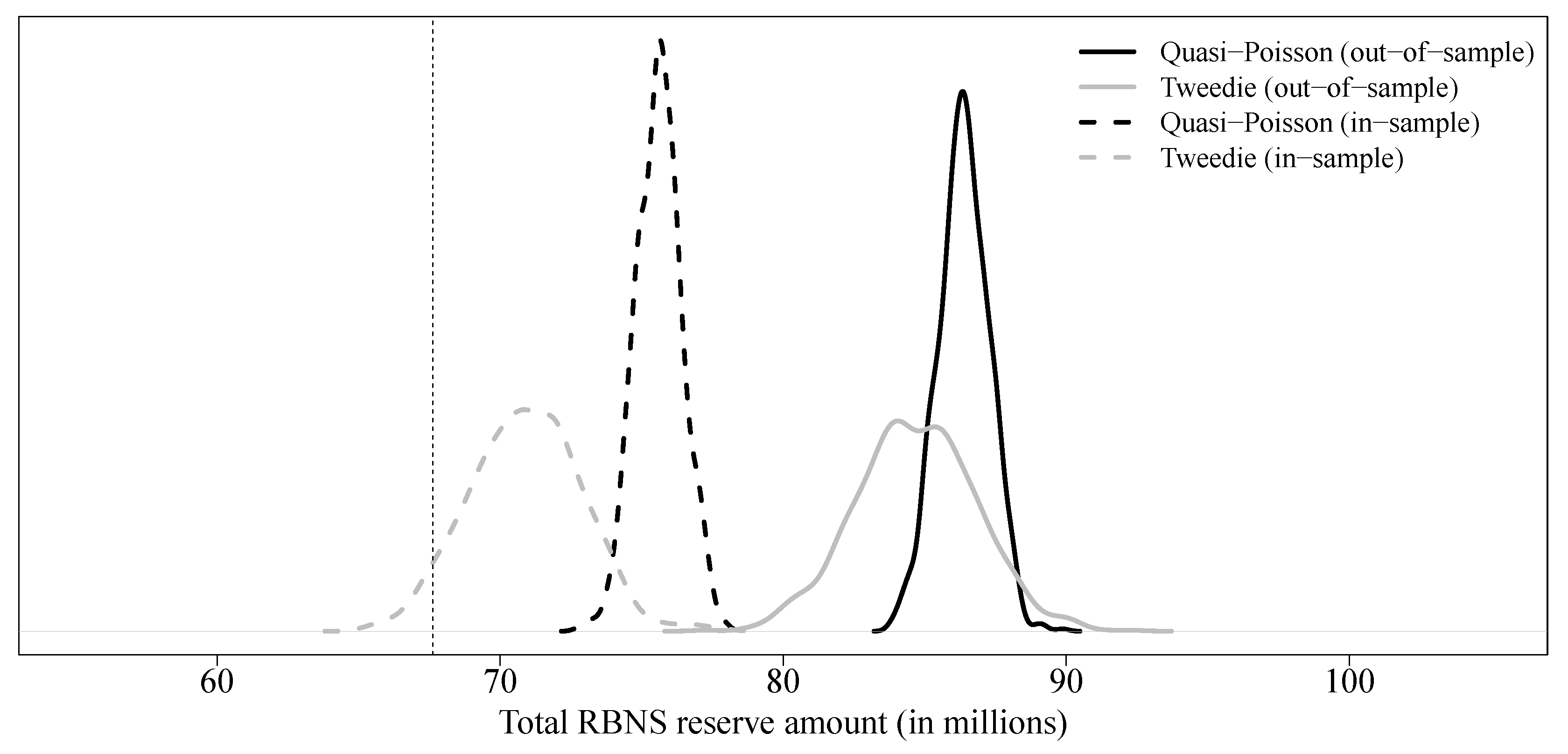
Results for individual GLM are displayed in

Table 5. Prediction results (RBNS) for individual generalized linear models using covariates.

Model		Assessment	$\mathbf{E}\left[\mathbf{Res}.\right]$	$\sqrt{\mathbf{Var}\left[\mathbf{Res}.\right]}$	${\mathit{q}}_{0.95}$	${\mathit{q}}_{0.99}$
Poisson		out-of-sample	86,411,734	9007	86,426,520	86,431,211
		in-sample	75,611,203	8655	75,625,348	75,631,190
Quasi-Poisson		out-of-sample	86,379,296	894,853	87,815,685	88,309,697
		in-sample	75,606,230	814,608	76,984,768	77,433,248
Tweedie		out-of-sample	84,693,529	2,119,280	88,135,187	90,011,542
		in-sample	70,906,225	1,994,004	74,098,686	75,851,991

Note: Because $70\%$ of the data is used for training and $30\%$ is used for testing, we use a factor of $7/3$ to correct in-sample predictions and make them comparable with out-of-sample predictions. The observed RBNS amount is $67,619,905.

, and predictive distributions for both quasi-Poisson and Tweedie GLM are shown in Figure 4. Predictive distribution for the Poisson GLM is omitted because it is the same as the quasi-Poisson model, but with a much smaller variance. Based on our dataset, we observe that the estimated value of the parameter associated to some covariates is particularly dependent on the database used to train the model, e.g., in the worst case, for the quasi-Poisson model, we observe $\widehat{\beta }=0.169$ ($0.091$) with the out-of-sample approach and $\widehat{\beta }=-1.009$ ($0.154$) with the in-sample approach. This can also be observed for many parameters of the model, as shown in Figure 5 for the quasi-Poisson model. These results were obtained by resampling from the training database and the quasi-Poisson model. Crosses and circles represent the estimated values of the parameters if the original training database is used, and the estimated values of the parameters if the validation database is used, respectively. On this graph, we observe that, for most of the parameters, the values estimated on the validation set are inaccessible when the model is adjusted on the training set. In Table 5, we display results for both in-sample and out-of-sample approaches. As the results shown in Figure 4 suggest, there are significant differences between the two approaches. Particularly, the reserves obtained from the out-of-sample approach are too high compared with the observed value. Although it is true that in practice, the training/validation set division is less relevant for an individual generalized linear model because the risk of overfitting is lower, this suggests that some caution is required in a context of loss reserving.

Out-of-sample results for XGBoost models are displayed in

Table 6. Prediction results (RBNS) for individual approaches (XGBoost) using covariates.

Model	$\mathbf{E}\left[\mathbf{Res}.\right]$	$\sqrt{\mathbf{Var}\left[\mathbf{Res}.\right]}$	${\mathit{q}}_{0.95}$	${\mathit{q}}_{0.99}$
Model A	73,204,299	3,742,971	79,329,916	82,453,032
Model B	14,339,470	6,723,608	25,757,061	30,643,369
Model C	67,655,960	2,411,739	71,708,313	73,762,242
Model D	68,313,731	4,176,418	75,408,868	78,517,966
Model E	67,772,822	2,387,476	71,722,744	73,540,516

Note: The observed RBNS amount is $67,619,905.

. For all models, the learning rate is around $10\%$, which means our models are quite robust to overfitting. We use a maximum depth of 3 for each tree. A higher value would make our model more complex but also less robust to overfitting. All those hyperparameters are obtained by cross-validation. Parameters ${\kappa }_C=0.8$ and ${\kappa }_D=0.8$ are obtained using cross-validation over a grid given by $\{0.6,0.7,0.8,0.9\}$.

Not surprisingly, we observe that model B is completely off the mark, underestimating the total reserve by a large amount. This confirms that the selection bias, at least in this example, is real and substantial.

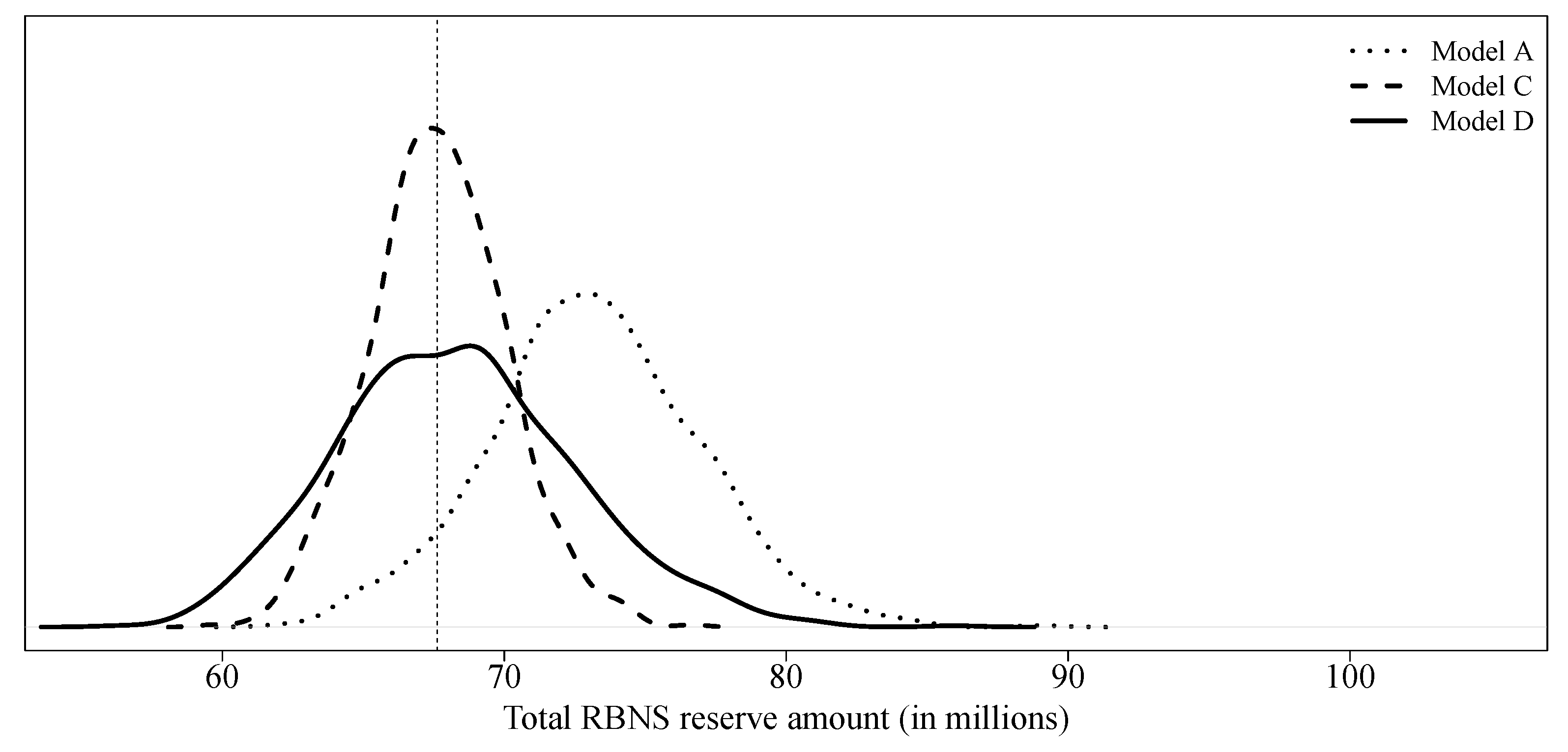
model C considers a collective model, i.e., without micro-covariates, to create pseudo-responses and uses all covariates available in order to predict final paid amounts. With a slightly lower expectation and variance, model C is quite similar to model A. Because the latter model uses real responses for its training, the method used for claim development appears to be reasonable. Model D uses an individual model, a quasi-Poisson GLM, using all covariates available to obtain both, pseudo-responses and final predictions. Again, results are similar to those of model A. In Figure 6 we compare the predictive distributions of model A, model C and model D.

Model E is identical to model C with the exception of dynamic variables whose value at the evaluation date was artificially replaced by the ultimate value. At least in this case study, the impact is negligible (see Figure 7). There would be no real interest in building a hierarchical model that allows, first, to develop the dynamic variables and, second, to use one XGBoost models to predict final paid amounts.

5. Conclusions

This paper studies the modeling of loss reserves for a property and casualty insurance company using micro-level approaches. More specifically, we apply generalized linear models and gradient boosting models designed to take into account the characteristics of each individual policyholder, as well as individual claims. We compare those models to classical approaches and show their performance on a detailed dataset from a Canadian insurance company. The choice of a gradient boosted decision-tree model is motivated by its strong performance for prediction on structured data. In addition, this type of algorithm requires very little data preprocessing, which is a notable benefit. The XGBoost algorithm was chosen for this analysis, mainly for its relatively short calculation time.

Through a case study, we mainly showed that

(1)

the censored nature of the data could strongly bias the loss reserving process; and

(2)

the use of a micro-level model based solely on generalized linear models could be unstable for loss reserving but an approach combining a macro-level (or a micro-level) model for the artificial completion of open claims and a micro-level gradient-boosting model represents an interesting approach for an insurance company.

The gradient boosting models presented in this paper allow insurers to compute a prediction for the total paid amount of each claim. Insurers might also be interested in modeling the payment schedule, namely to predict the date and the amount of each individual payment. Moreover, we know that payments for parties belonging to the same claim are not independent and are positively correlated. Therefore, one could extend the model by adding a dependence structure between parties. The same principle could be applied with the different types of coverage (medical and rehabilitation, income replacement, etc.). Dynamic covariates can change over time, which makes their future value random. In this work, we assumed that their value will not change after the evaluation date and we checked that the impact was not very high. However, for a different database, this could have a significant impact on the results. A possible refinement would be to build a hierarchical model that first predicts the ultimate values of dynamic covariates before inputting them in the gradient boosting algorithm.

In recent years, several new individual approaches have been proposed. It will be interesting, in a future case study, to compare the results obtained, on the same database, using these different methods. Finally, in this case study, we always consider predictive distributions to compare models. One might wonder why we do not use criteria often used in machine learning such as the root mean squared error (RMSE) or the mean absolute error (MAE). The reason lies, at least in part, in the fact that the database used in this work contains numerous small (or zero) claims and very few large claims. Therefore, because RMSE and MAE are symmetric error functions, they favor models that predict low reserves. Expectile regression is an avenue that is being explored to overcome this weakness.

References

- Antonio, Katrien, and Richard Plat. 2014. Micro-level stochastic loss reserving for general insurance. Scandinavian Actuarial Journal 7: 649–69. [Google Scholar] [CrossRef]
- Arjas, Elja. 1989. The claims reserving problem in non-life insurance: Some structural ideas. ASTIN Bulletin 19: 140–52. [Google Scholar] [CrossRef]
- Baudry, Maximilien, and Christian Y. Robert. 2017. Non Parametric Individual Claim Reserving in Insurance. Working paper. [Google Scholar]
- Breiman, Leo, Friedman Jerome, Olshen Richard, and Stone Charles. 1984. Classification and Regression Trees. Wadsworth Statistics/Probability Series; New York: Routledge. [Google Scholar]
- Buhlmann, Hans, Rene Schnieper, and Erwin Straub. 1980. Claims reserves in casualty insurance based on a probabilistic model. Bulletin of the Association of Swiss Actuaries 80: 21–45. [Google Scholar]
- Charpentier, Arthur, and Mathieu Pigeon. 2016. Macro vs. micro methods in non-life claims reserving (an econometric perspective). Risks 4: 12. [Google Scholar] [CrossRef]
- Chen, Tianqi, and Carlos Guestrin. 2016. Xgboost: A scalable tree boosting system. Paper presented at 22nd ACM SIGKDD International Conference on Knowledge Discovery and Data Mining, San Francisco, CA, USA, August 13–17; pp. 785–94. [Google Scholar]
- De Jong, Piet, and Gillian Z. Heller. 2008. Generalized Linear Models for Insurance Data. Cambridge: Cambridge University Press. [Google Scholar]
- England, Peter D., and Richard J. Verrall. 2002. Stochastic claims reserving in general insurance. British Actuarial Journal 8: 443–544. [Google Scholar] [CrossRef]
- Friedman, Jerome H. 2001. Greedy function approximation: A gradient boosting machine. Annals of Statistics 29: 1189–232. [Google Scholar] [CrossRef]
- Gabrielli, Andrea, Ronald Richman, and Mario V. Wüthrich. 2019. Neural Network Embedding of the Over-Dispersed Poisson Reserving Model. Scandinavian Actuarial Journal 2019: 1–29. [Google Scholar] [CrossRef]
- Haastrup, Svend, and Elja Arjas. 1996. Claims reserving in continuous time; a nonparametric bayesian approach. ASTIN Bulletin 26: 139–64. [Google Scholar] [CrossRef]
- Hachemeister, Charles. 1980. A stochastic model for loss reserving. Transactions of the 21st International Congress of Actuaries 1: 185–94. [Google Scholar]
- Hesselager, Ole. 1994. A Markov model for loss reserving. ASTIN Bulletin 24: 183–93. [Google Scholar] [CrossRef]
- Hiabu, Munir, Margraf Carolin, Martínez-Miranda Maria, and Nielsen Jens Perch. 2016. The link between classical reserving and granular reserving through double chain ladder and its extensions. British Actuarial Journal 21: 97–116. [Google Scholar] [CrossRef]
- Huang, Jinlong, Chunjuan Qiu, and Xianyi Wu. 2015. Stochastic loss reserving in discrete time: Individual vs. aggregate data models. Communications in Statistics—Theory and Methods 44: 2180–206. [Google Scholar] [CrossRef]
- Jewell, William S. 1989. Predicting IBNYR events and delays. ASTIN Bulletin 19: 25–55. [Google Scholar] [CrossRef]
- Larsen, Christian Roholte. 2007. An individual claims reserving model. ASTIN Bulletin 37: 113–32. [Google Scholar] [CrossRef]
- Lopez, Olivier, Xavier Milhaud, and Pierre-E. Thérond. 2016. Tree-based censored regression with applications in insurance. Electronic Journal of Statistics 10: 2685–716. [Google Scholar] [CrossRef]
- Mack, Thomas. 1993. Distribution-free calculation of the standard error of chain ladder reserve estimates. ASTIN Bulletin: The Journal of the IAA 23: 213–25. [Google Scholar] [CrossRef]
- Norberg, Ragnar. 1986. A contribution to modeling of IBNR claims. Scandinavian Actuarial Journal 1986: 155–203. [Google Scholar] [CrossRef]
- Norberg, Ragnar. 1993. Prediction of outstanding liabilities in non-life insurance. ASTIN Bulletin 23: 95–115. [Google Scholar] [CrossRef]
- Norberg, Ragnar. 1999. Prediction of outstanding liabilities. II Model variations and extensions. ASTIN Bulletin 29: 5–25. [Google Scholar] [CrossRef]
- Pigeon, Mathieu, Katrien Antonio, and Michel Denuit. 2013. Individual loss reserving with the multivariate skew normal framework. ASTIN Bulletin 43: 399–428. [Google Scholar] [CrossRef]
- Taylor, Greg, Gráinne McGuire, and James Sullivan. 2008. Individual claim loss reserving conditioned by case estimates. Annals of Actuarial Science 3: 215–56. [Google Scholar] [CrossRef]
- Wüthrich, Mario V. 2018. Machine learning in individual claims reserving. Scandinavian Actuarial Journal. in press. [Google Scholar] [CrossRef]
- Wüthrich, Mario V., and Michael Merz. 2008. Stochastic Claims Reserving Methods in Insurance. Zürich and Tübigen: Wiley. [Google Scholar]
- Zhao, Xiaobing, and Xian Zhou. 2010. Applying copula models to individual claim loss reserving methods. Insurance: Mathematics and Economics 46: 290–99. [Google Scholar] [CrossRef]
- Zhao, Xiaobing, Xian Zhou, and Jing Long Wang. 2009. Semiparametric model for prediction of individual claim loss reserving. Insurance: Mathematics and Economics 45: 1–8. [Google Scholar] [CrossRef]
Figure 1.
Development of claim k.
Figure 2.
(a) Status of claims of incurred amounts on 31 December 2016; (b) Means and standard deviations of incurred amounts on 31 December 2016.
Figure 3.
Comparison of predictive distributions (incurred but not reported (IBNR) + reported but not settled (RBNS)) for collective models.
Figure 4.
Predictive distributions (RBNS) for individual GLM with covariates.
Figure 5.
Means and confidence intervals for all parameters of the model.
Figure 6.
Predictive distributions (RBNS) for XGBoost models A, C and D.
Figure 7.
Comparison of predictive distributions for models E and C.