Quantile Regression with Telematics Information to Assess the Risk of Driving above the Posted Speed Limit


Abstract
:1. Objective
2. Background
3. Methods
3.1. Quantile Regression
3.2. The Data
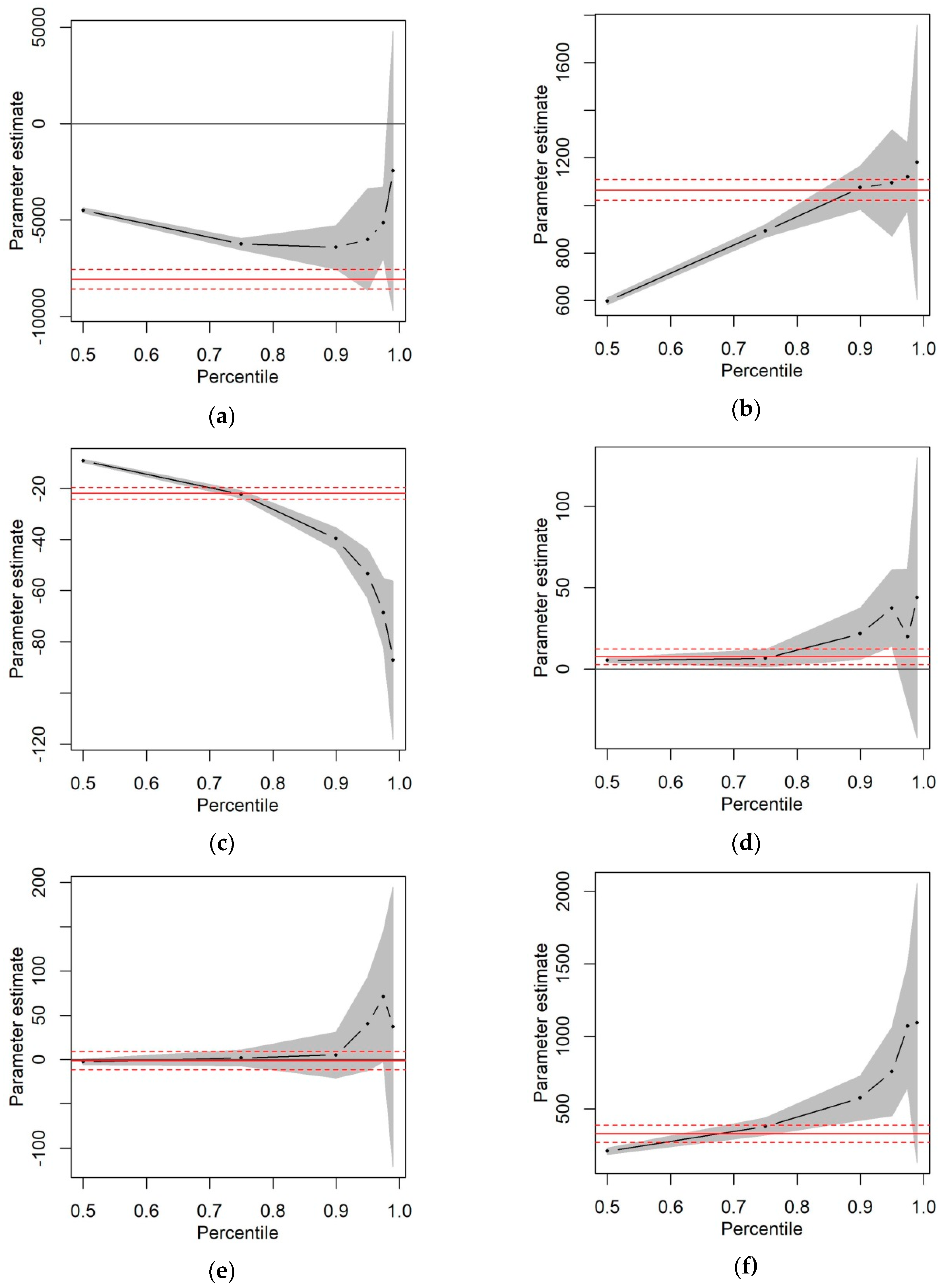
4. Results
5. Conclusions
Author Contributions
Funding
Conflicts of Interest
Appendix A

| Parameter Estimate (p-Value) | |
|---|---|
| Intercept | 0.6397 (<0.0001) |
| Km_1000 | 0.0292 (<0.0001) |
| Km_10002 | 0.0035 (<0.0001) |
| Pkdr_vurba | −0.0137 (<0.0001) |
| Pkdr_nocturn | 0.0018 (0.485) |
| Age | −0.0079 (0.149) |
| Gender | 0.2295 (<0.0001) |
| R2 | 43.20% |
| 50th Percentile (p-Value) | 75th Percentile (p-Value) | 90th Percentile (p-Value) | 95th Percentile (p-Value) | 97.5th Percentile (p-Value) | 99th Percentile (p-Value) | |
|---|---|---|---|---|---|---|
| Intercept | 0.1812 (0.0003) | 0.3845 (<0.0001) | 0.3681 (0.0805) | 0.4940 (0.0643) | 0.1147 (0.7889) | 0.8439 (0.1271) |
| Km_1000 | 0.0113 (0.0399) | 0.0257 (0.0010) | 0.0595 (0.0001) | 0.0839 (<0.0001) | 0.0887 (0.0084) | 0.0632 (0.0243) |
| Km_10002 | 0.0035 (<0.0001) | 0.0056 (<0.0001) | 0.0079 (<0.0001) | 0.0087 (<0.0001) | 0.0107 (<0.0001) | 0.0138 (<0.0001) |
| Pkdr_vurba | −0.0031 (<0.0001) | −0.0082 (<0.0001) | −0.0136 (<0.0001) | −0.0177 (<0.0001) | −0.0200 (<0.0001) | −0.0248 (<0.0001) |
| Pkdr_nocturn | 0.0023 (0.0164) | 0.0010 (0.4777) | −0.0022 (0.6037) | 0.0028 (0.6140) | 0.0055 (0.5539) | 0.0095 (0.4052) |
| Age | −0.0027 (0.1316) | −0.0001 (0.9749) | 0.0143 (0.0623) | 0.0216 (0.0266) | 0.0480 (0.0019) | 0.0416 (0.0725) |
| Gender | 0.1132 (<0.0001) | 0.1734 (<0.0001) | 0.1975 (<0.0001) | 0.1510 (0.0082) | 0.1428 (0.1198) | 0.2360 (0.1646) |
| Goodness-of-fit criterion | 23.62% | 33.45% | 43.70% | 49.62% | 54.10% | 59.67% |
| Driver 1 | Driver 2 | Driver 3 | |
|---|---|---|---|
| Km | 12,000 | 8000 | 5500 |
| Pkdr_vurba | 80 | 75 | 80 |
| Pkdr_noctur | 14 | 11 | 10.5 |
| Age | 25 | 25 | 25 |
| Gender | 1 | 1 | 1 |
| Estimated conditional percentile 1 | 45th | 78th | 96th |
References
- Ayuso, Mercedes, Montserrat Guillen, and Ana Maria Pérez-Marín. 2014. Time and distance to first accident and driving patterns of young drivers with pay-as-you-drive insurance. Accident Analysis and Prevention 73: 125–31. [Google Scholar] [CrossRef] [PubMed]
- Ayuso, Mercedes, Montserrat Guillen, and Ana Maria Pérez-Marín. 2016a. Telematics and gender discrimination: Some usage-based evidence on whether men’s risk of accident differs from women’s. Risks 4: 10. [Google Scholar] [CrossRef]
- Ayuso, Mercedes, Montserrat Guillen, and Ana Maria Pérez-Marín. 2016b. Using GPS data to analyse the distance travelled to the first accident at fault in pay-as-you-drive insurance. Transportation Research Part C Emerging Technologies 68: 160–67. [Google Scholar] [CrossRef]
- Boucher, Jean-Philippe, Ana Maria Pérez-Marín, and Miguel Santolino. 2013. Pay-as-you-drive insurance: The effect of the kilometers on the risk of accident. Anales del Instituto de Actuarios Españoles 19: 135–54. [Google Scholar]
- Dissanayake, Susanda, and Jian John Lu. 2002. Factors influential in making an injury severity difference to older drivers involved in fixed object-passenger car crashes. Accident Analysis and Prevention 34: 609–18. [Google Scholar] [CrossRef]
- Gao, Guangyuan, and Mario V. Wüthrich. 2019. Convolutional neural network classification of telematics car driving data. Risks 7: 6. [Google Scholar] [CrossRef]
- Gao, Guangyuan, Shengwang Meng, and Mario V. Wüthrich. 2019a. Claims frequency modeling using telematics car driving data. Scandinavian Actuarial Journal 2: 143–62. [Google Scholar] [CrossRef]
- Gao, Guangyuan, Mario V. Wüthrich, and Hanfang Yang. 2019b. Evaluation of driving risk at different speeds. Insurance: Mathematics and Economics 88: 108–19. [Google Scholar] [CrossRef]
- Guillen, Montserrat, Jens Perch Nielsen, Mercedes Ayuso, and Ana Maria Pérez-Marín. 2019. The use of telematics devices to improve automobile insurance rates. Risk Analysis 39: 662–72. [Google Scholar] [CrossRef]
- Hewson, Paul James. 2008. Quantile regression provides a fuller analysis of speed data. Accident Analysis and Prevention 40: 502–10. [Google Scholar] [CrossRef]
- Jun, Jungwook, Jennifer Ogle, and Randall Guensler. 2007. Relationships between crash involvement and temporal-spatial driving behavior activity patterns: Use of data for vehicles with global positioning systems. Transportation Research Record 2019: 246–55. [Google Scholar] [CrossRef]
- Jun, Jungwook, Randall Guensler, and Jennifer Ogle. 2011. Differences in observed speed patterns between crash-involved and crash-not-involved drivers: Application of in-vehicle monitoring technology. Transportation Research Part C Emerging Technologies 19: 569–78. [Google Scholar] [CrossRef]
- Koenker, Roger, and Kevin Hallock. 2001. Quantile regression. Journal of Economic Perspectives 15: 143–56. [Google Scholar] [CrossRef]
- Koenker, Roger, and José A. F. Machado. 1999. Goodness of fit and related inference processes for quantile regression. Journal of the American Statistical Association 94: 1296–310. [Google Scholar] [CrossRef]
- Koenker, Roger, Stephen Portnoy, Pin Tian Ng, Achim Zeisleis, Philip Grosjean, and Brian D. Ripley. 2018. Package ‘Quantreg’. R Package Version 5.38. Available online: https://cran.r-project.org/web/packages/quantreg/quantreg.pdf (accessed on 28 June 2019).
- Ossiander, Eric M., and Peter Cummings. 2002. Freeway speed limits and traffic fatalities in Washington State. Accident Analysis and Prevention 34: 13–18. [Google Scholar] [CrossRef]
- Paefgen, Johannes, Thorsten Staake, and Elgar Fleisch. 2014. Multivariate exposure modeling of accident risk: Insights from pay-as-you-drive insurance data. Transportation Research Part A Policy and Practice 61: 27–40. [Google Scholar] [CrossRef]
- Pérez-Marín, Ana Maria, and Montserrat Guillen. 2019. Semi-autonomous vehicles: Usage-based data evidences of what could be expected from eliminating speed limit violations. Accident Analysis and Prevention 123: 99–106. [Google Scholar] [CrossRef] [PubMed]
- Pérez-Marín, Ana Maria, Mercedes Ayuso, and Montserrat Guillen. 2019. Do young insured drivers slow down after suffering an accident? Transportation Research Part F: Traffic Psychology and Behaviour 62: 690–99. [Google Scholar] [CrossRef]
- Pilkington, Paul, and Sanjay Kinra. 2005. Effectiveness of speed cameras in preventing road traffic collisions and related casualties: Systematic review. BMJ 330: 331–34. [Google Scholar] [CrossRef]
- Taylor, M., A. Baruya, and J. Kennedy. 2002. The Relationship between Speed and Accidents on Rural Single-Carriageway Roads. TRL Report TRL511. Crowthorne: Transport Research Laboratory. [Google Scholar]
- Vernon, Donald, Lawrence J. Cook, Katherine J. Peterson, and J. Michael Dean. 2004. Effect of the repeal of the national maximum speed limit law on occurrence of crashes, injury crashes, and fatal crashes on Utah highways. Accident Analysis and Prevention 36: 223–29. [Google Scholar] [CrossRef]
- Wilson, Cecilia, Charlene Willis, Joan K. Hendrikz, and Nicholas Bellamy. 2006. Speed enforcement detection devices for preventing road traffic injuries. Cochrane Database of Systematic Reviews Issue 2: CD004607. [Google Scholar] [CrossRef]
- Yu, Rongjie, and Mohamed Abdel-Aty. 2014. Using hierarchical Bayesian binary probit models to analyze crash injury severity on high speed facilities with real-time traffic data. Accident Analysis and Prevention 62: 161–67. [Google Scholar] [CrossRef] [PubMed]
- Yu, Keming, Zudi Lu, and Julian Stander. 2003. Quantile regression: Applications and current research areas. Journal of the Royal Statistical Society D 52: 331–50. [Google Scholar] [CrossRef]


| Variable | Description |
|---|---|
| Tolerkm | Number of kilometers driven at speeds above the posted limit during 2010. |
| Km | Total number of kilometers driven during 2010. |
| Lnkm | Logarithm of the total number of kilometers driven during 2010. |
| Pkdr_vurba | % of kilometers driven on urban roads during 2010. |
| Pkdr_nocturn | % of kilometers driven at night (between midnight and 6 am.) during 2010. |
| Age | Age of the driver at the beginning of 2010. |
| Gender | 1 = Male, 0 = Female |
| Variable | Min | 1st Qu | Median | Mean | 3rd Qu | Max | St. Dev. | Skewness |
|---|---|---|---|---|---|---|---|---|
| Tolerkm | 0.00 | 282.40 | 689.20 | 1398.20 | 1701.60 | 23,500.20 | 1995.37 | 3.64 |
| Km | 0.69 | 7530.56 | 11,697.82 | 13,063.71 | 17,337.00 | 57,756.98 | 7715.80 | 1.08 |
| Lnkm | −0.37 | 8.93 | 9.37 | 9.27 | 9.76 | 10.96 | 0.75 | −1.87 |
| Pkdr_vurba | 0.00 | 15.60 | 23.39 | 26.29 | 34.32 | 100.00 | 14.18 | 1.03 |
| Pkdr_nocturn | 0.00 | 2.48 | 5.31 | 7.02 | 9.84 | 78.56 | 6.13 | 1.67 |
| Age | 18.11 | 22.66 | 24.63 | 24.78 | 26.88 | 35.00 | 2.82 | 0.11 |
| Parameter Estimate (p-Value) | |
|---|---|
| Intercept | −8082.506 (<0.0001) |
| Lnkm | 1064.506 (<0.0001) |
| Pkdr_vurba | −21.868 (<0.0001) |
| Pkdr_nocturn | 7.536 (0.0101) |
| Age | −1.131 (0.8565) |
| Gender | 328.009 (<0.0001) |
| R2 | 25.96% |
| 50th Percentile (p-Value) | 75th Percentile (p-Value) | 90th Percentile (p-Value) | 95th Percentile (p-Value) | 97.5th Percentile (p-Value) | 99th Percentile (p-Value) | |
|---|---|---|---|---|---|---|
| Intercept | −4496.53 (<0.0001) | −6250.34 (<0.0001) | −6418.11 (<0.0001) | −6009.63 (<0.001) | −5137.24 (<0.0001) | −2451.17 0.5780 |
| Lnkm | 597.60 (<0.0001) | 892.80 (<0.0001) | 1074.66 (<0.0001) | 1094.57 (<0.0001) | 1119.94 (<0.0001) | 1180.21 (<0.001) |
| Pkdr_vurba | −9.19 (<0.0001) | −22.26 (<0.0001) | −39.59 (<0.0001) | −53.44 (<0.0001) | −68.58 (<0.0001) | −87.12 (<0.0001) |
| Pkdr_nocturn | 5.41 (<0.0001) | 6.71 (0.0363) | 21.76 (0.0226) | 37.49 (0.0086) | 20.01 (0.4266) | 43.86 (0.4014) |
| Age | −2.56 (0.1632) | 1.84 (0.7298) | 5.16 (0.7419) | 40.29 (0.2086) | 71.28 (0.1094) | 36.87 (0.7009) |
| Gender | 206.76 (<0.0001) | 377.94 (<0.0001) | 574.08 (<0.0001) | 755.87 (<0.0001) | 1070.06 (<0.0001) | 1091.38 (0.0624) |
| Goodness-of-fit criterion | 14.19% | 18.26% | 20.23% | 20.27% | 20.56% | 20.06% |
| Driver 1 | Driver 2 | Driver 3 | |
|---|---|---|---|
| Km | 12,000 | 8000 | 5500 |
| Pkdr_vurba | 80 | 75 | 80 |
| Pkdr_noctur | 14 | 11 | 10.5 |
| Age | 25 | 25 | 25 |
| Gender | 1 | 1 | 1 |
| Estimated conditional percentile 1 | 50th | 75th | 90th |
© 2019 by the authors. Licensee MDPI, Basel, Switzerland. This article is an open access article distributed under the terms and conditions of the Creative Commons Attribution (CC BY) license (http://creativecommons.org/licenses/by/4.0/).
Share and Cite
Pérez-Marín, A.M.; Guillen, M.; Alcañiz, M.; Bermúdez, L. Quantile Regression with Telematics Information to Assess the Risk of Driving above the Posted Speed Limit. Risks 2019, 7, 80. https://doi.org/10.3390/risks7030080
Pérez-Marín AM, Guillen M, Alcañiz M, Bermúdez L. Quantile Regression with Telematics Information to Assess the Risk of Driving above the Posted Speed Limit. Risks. 2019; 7(3):80. https://doi.org/10.3390/risks7030080
Chicago/Turabian StylePérez-Marín, Ana M., Montserrat Guillen, Manuela Alcañiz, and Lluís Bermúdez. 2019. "Quantile Regression with Telematics Information to Assess the Risk of Driving above the Posted Speed Limit" Risks 7, no. 3: 80. https://doi.org/10.3390/risks7030080
APA StylePérez-Marín, A. M., Guillen, M., Alcañiz, M., & Bermúdez, L. (2019). Quantile Regression with Telematics Information to Assess the Risk of Driving above the Posted Speed Limit. Risks, 7(3), 80. https://doi.org/10.3390/risks7030080