1. Introduction
Social media communication is crucial in all sectors of the population’s life. Companies use social media to massively promote products and services, while people use them to transmit experiences and opinions. Natural Language Processing (NLP) and Text Mining have been of great interest in exploring this source of textual communication to generate information about mass behavior, thoughts, and emotions on a wide variety of topics, such as product reviews [
1], political trends [
2], and stock market sentiment [
3]. During the Coronavirus pandemic, people expressed how they experienced the consequences of quarantine, the way it altered the daily rhythm of life, and how they changed their day-to-day activities.
Among the most used social media during the pandemic was Twitter, which at the time functioned as a freely accessible universal microexpression tool. This made it an ideal platform to capture the population’s feelings during this historic moment. Many studies have been presented that analyze various aspects of the epidemic, some of them on Twitter and mainly in English.
This article presents the work carried out to study the emotional impact of COVID-19 on the Mexican population. The MIOPERS platform responded to UNAM’s initiative to develop models for the analysis and visualization of information that support strategic decision-making, especially during lockdown. During the pandemic, there were two main motivations for starting such work: (a) to evaluate people’s behavior, moods, and popularity of the measures given by the government and (b) to monitor users with possible symptoms.
This initiative, which covers two years (2020–2022), the duration of the pandemic, allowed a compilation of many tweets related to COVID-19. This facilitated the study of topic-related lexicon, mentions, and hashtags, which in turn served as a basis for studying other important NLP topics, such as sentiment analysis.
This article focuses on developing a specific corpus for polarity analysis of COVID-19, the SENT-COVID corpus, taking a subset of the tweets collected by the Miopers system during the pandemic. Furthermore, polarity classification experiments are performed, applying both traditional ML and DL methods. To do this, the article follows the structure explained below. Related work is discussed in
Section 2, especially on sentiment analysis in social networks or specifically oriented to the topic of COVID-19.
Section 3 explains the compilation of the corpus, the annotation protocol, and the agreement results. The methodology that has been followed to carry out the analysis is described in
Section 4, including pre-processing, forms of text representation, and algorithms used. The results are presented and discussed in
Section 5. The article concludes with the conclusions in
Section 6.
2. Related Work
Numerous toolkits are available to process textual data, which makes complex NLP tasks more accessible with user-friendly interfaces. In the context of sentiment analysis, several researchers have used libraries such as TextBlob, VADER, and Pysentimiento, among others. TextBlob and VADER have the advantage of not requiring training data, as it is a lexicon-based approach. Therefore, they have been popular tools for analyzing comments on social networks, such as tweets [
4,
5,
6,
7,
8], youtube [
9,
10,
11,
12,
13] or Reddit [
14,
15,
16,
17] comments. Although the lexicon-based approach is suitable for general use, its main limitation lies in its difficulty adapting to changing contexts and linguistic uses [
18]. Examples are texts such as tweets that have a lively and casual tone [
19]. In addition, if we look at those related to COVID-19, we find new terms associated with the phenomenon. Additionally, since TextBlob and VADER were designed mainly for English-language texts, they may not be as effective when used in texts in other languages. Therefore, a toolkit for analyzing text sentiments and emotions in a wide range of languages is the Pysentimiento library, which offers support for multiple languages [
20,
21,
22], including Spanish [
23,
24]. Furthermore, Pysentimiento uses state-of-the-art machine learning models, such as BERT (Bidirectional Encoder Representations from Transformers) models, for sentiment analysis. However, this requires more computing resources than TextBlob or VADER.
From the beginning of the quarantine period, several researchers studied social media information to measure people’s feelings about their situation during the COVID-19 pandemic [
25]. This has been done considering the language and domain of the comments posted on the different social platforms [
26]. Many studies have used TextBlob, VADER, and Pysentimiento tools for sentiment analysis on social networks [
6,
23,
27,
28,
29,
30,
31]. Moreover, machine learning approaches have been widely adopted to categorize sentiments into two (negative and positive) or three classes (positive, negative, and neutral). For example, Long Short Term Memory (LSTM) recurrent neural network has been used in Reddit comments, which allows for 81.15% accuracy [
32].
Chunduri and Perera [
33] have used advanced deep learning models, such as Spiking Neural Networks (SNN), for polarity-based classification. SNNs encompass what is known as brain-based computing, and attempt to mimic the distinctive functionalities of the human brain in terms of energy efficiency, computational power, and robust learning. Although they report 100% accuracy with their model, their main claim is that SNNs have lower energy consumption than ANNs.
For public tweets related to COVID-19, the TClustVID model [
34] was developed, achieving a high accuracy of 98.3%.
Researchers have also analyzed the performance of language models for sentiment analysis in Spanish. Specifically, for the COVID-19 tweet polarity, Contreras et al. [
35] found that pre-trained BERT models in Spanish (BETO), with domain-adjusted, have achieved a high accuracy of 97% in training and 81% in testing. Such performance was the best compared to multilingual BERT models and other classification methods such as Decision Trees, Support Vector Machines, Naive Bayes, and Logistic Regression.
Research has focused not only on creating computational models for text classification but also on annotated datasets, which help to train and evaluate models in supervised learning approaches. An example is COVIDSENTI [
36], which consists of 90,000 COVID-19-related English-language tweets collected in the early stage of the pandemic from February to March 2020. Each tweet has been labeled as positive, negative, or neutral. Furthermore, state-of-the-art BERT models have been applied to the data to obtain a high precision of 98.3%.
For sentiment analysis, several corpora of annotated tweets related to COVID-19, mainly in English, have been released [
36,
37,
38,
39,
40]. However, since the behavior of social media users also varies with language [
41], having datasets in various languages besides English is crucial. Therefore, efforts have been made to compile multilingual corpora [
42,
43] as well as language-specific datasets such as Portuguese [
44,
45], Arabic [
46,
47], French [
48], among others [
49,
50,
51]. For the Spanish language, there are annotated tweet datasets for tasks such as hate speech detection [
52], aggression detection [
53], LGBT-phobia detection [
54], and automatic stance detection [
55], among others. However, to our knowledge, there is no manually annotated public corpus for the sentiment polarity of COVID-19-related tweets in Spanish. Given that research tends to use an automatic labeling process. Like the work by Contreras mentioned above [
35]. Therefore, we present a corpus with a manual labeling process and an annotation guideline. Furthermore, we provided an extensive analysis of the agreement between the annotators.
6. Conclusions
This paper presents SENT-COVID, a Twitter corpus of COVID-19 in Mexican Spanish manually annotated with polarity. We have designed several classification experiments with this resource using ready-to-use libraries, classical machine learning methods, and deep learning approaches based on transformers.
In light of the temporal context surrounding the compilation and presentation of our corpus, it is crucial to emphasize the importance of its value in hindsight. While we acknowledge that the corpus’s arrival may seem overdue, We firmly assert that it remains relevant to our understanding of linguistic patterns and public discourse. As a historical archive of Mexican Spanish tweets during the pandemic, our corpus offers unique insights into the evolution of societal responses, linguistic shifts, and sentiment fluctuations over time. Despite the availability of other resources, the retrospective nature of our corpus provides researchers with an invaluable opportunity to conduct comparative analyses, trace the trajectory of linguistic trends, and evaluate the enduring impact of COVID-19 discourse on societal norms and behaviors. Furthermore, we emphasize the corpus’s potential to complement existing datasets and tools, enriching interdisciplinary research endeavors in fields such as linguistics, public health communication, and computational social science.
Given the experiments, we observe that, among the black-box libraries, neither TextBlob nor Vader demonstrated satisfactory performance, probably due to the difficulty of obtaining a suitable lexicon in Spanish. In contrast, Pysentimiento exhibits better performance because it employs machine learning models trained on large Spanish corpora to classify text into sentiment categories such as positive, negative, or neutral, and to detect emotions such as joy, anger, sadness, and fear with higher accuracy and contextual understanding. By leveraging machine learning techniques, PySentimiento can capture the nuances of sentiment expressed in Spanish text more effectively, overcoming the limitations faced by lexicon-based approaches like TextBlob and Vader.
The supervised models have revealed that contrary to our initial expectations, removing common words is not as effective as we had thought. However, the models showed that including a broader range of features and observations improved performance without requiring too much computing power. The dimension reduction models managed to improve the prediction results with fewer features, so we can conclude that it is a viable alternative to tackle this problem. However, there is still much to explore. Furthermore, the penalty parameter selection did not make a major difference as expected, neither Ridge nor Lasso regularization, and it performed almost the same as with the default parameters.
The results of the Doc2Vec models did not meet the expectations, as they could not outperform basic BoW models. Additionally, training these models is associated with a higher computational cost.
Finally, pre-trained BERT models yielded the best results. However, they are the most expensive in terms of computational cost. Additionally, it is difficult to perform different tests since cross-validation is difficult. Therefore, the parameters and configuration settings must be chosen based on another criterion. Despite these challenges, for datasets that are not too large, pre-trained BERT models are the most suitable choice.
Author Contributions
Conceptualization, H.G.-A., G.B.-E. and G.S.; methodology, H.G.-A., G.B.-E. and G.S.; software, H.G.-A. and J.-C.B.; validation, G.B.-E., G.S. and W.Á.; formal analysis, H.G.-A. and J.-C.B.; investigation, H.G.-A. and J.-C.B.; resources, H.G.-A., G.B.-E. and G.S.; data curation, H.G.-A., J.-C.B. and W.Á.; writing—original draft preparation, H.G.-A. and J.-C.B.; writing—review and editing, G.B.-E., G.S. and W.Á.; visualization, J.-C.B. and W.Á.; supervision, H.G.-A.; project administration, H.G.-A.; funding acquisition, H.G.-A., G.B.-E. and G.S. All authors have read and agreed to the published version of the manuscript.
Funding
This research was funded by CONAHCYT project number CF-2023-G-64, and by PAPIIT projects TA101722 and IN104424.
Institutional Review Board Statement
Not applicable.
Informed Consent Statement
Not applicable.
Data Availability Statement
SENT-COVID corpus can be found here:
https://github.com/GIL-UNAM/SENT-COVID (accessed on 20 February 2024). The dataset is licensed under CC0, so it is open data. If the data are used, we would appreciate citing this article as the corpus descriptor.
Acknowledgments
Authors thank CONAHCYT for the computing resources provided through the Deep Learning Platform for Language Technologies of the INAOE Supercomputing Laboratory, as well as Gabriel Castillo for the computing services.
Conflicts of Interest
The authors declare no conflict of interest.
Abbreviations
The following abbreviations are used in this manuscript:
| NLP | Natural Language Processing |
| ML | Machine Learning |
| DL | Deep Learning |
| LSTM | Long Short Term Memory |
| BERT | Bidirectional Encoder Representations from Transformers |
| IAA | Inter-Annotator Agreement |
| BoW | Bag of Words |
| Tf-Idf | Term Frequency-Inverse Document Frequency |
| MLP | Multilayer Perceptron |
| CBOW | Continuous Bag of Words |
| DBOW | Distributed Bag of Words |
| DM | Distributed Memory |
| NB | Naïve Bayes |
| SVM | Support Vector Machines |
References
- Shivaprasad, T.; Shetty, J. Sentiment analysis of product reviews: A review. In Proceedings of the 2017 International Conference on Inventive Communication and Computational Technologies (ICICCT), Coimbatore, India, 10–11 March 2017; pp. 298–301. [Google Scholar]
- Das, A.; Gunturi, K.S.; Chandrasekhar, A.; Padhi, A.; Liu, Q. Automated pipeline for sentiment analysis of political tweets. In Proceedings of the 2021 International Conference on Data Mining Workshops (ICDMW), Auckland, New Zealand, 7–10 December 2021; pp. 128–135. [Google Scholar]
- Man, X.; Luo, T.; Lin, J. Financial sentiment analysis (fsa): A survey. In Proceedings of the 2019 IEEE International Conference on Industrial Cyber Physical Systems (ICPS), Taipei, Taiwan, 6–9 May 2019; pp. 617–622. [Google Scholar]
- Shelar, A.; Huang, C.Y. Sentiment Analysis of Twitter Data. In Proceedings of the 2018 International Conference on Computational Science and Computational Intelligence (CSCI), Las Vegas, NV, USA, 12–14 December 2018; pp. 1301–1302. [Google Scholar] [CrossRef]
- Zahoor, S.; Rohilla, R. Twitter Sentiment Analysis Using Lexical or Rule Based Approach: A Case Study. In Proceedings of the 2020 8th International Conference on Reliability, Infocom Technologies and Optimization (Trends and Future Directions) (ICRITO), Noida, India, 4–5 June 2020; pp. 537–542. [Google Scholar] [CrossRef]
- Nair, A.J.; G, V.; Vinayak, A. Comparative study of Twitter Sentiment On COVID-19 Tweets. In Proceedings of the 2021 5th International Conference on Computing Methodologies and Communication (ICCMC), Erode, India, 8–10 April 2021; pp. 1773–1778. [Google Scholar] [CrossRef]
- Diyasa, I.G.S.M.; Mandenni, N.M.I.M.; Fachrurrozi, M.I.; Pradika, S.I.; Manab, K.R.N.; Sasmita, N.R. Twitter Sentiment Analysis as an Evaluation and Service Base On Python Textblob. IOP Conf. Ser. Mater. Sci. Eng. 2021, 1125, 012034. [Google Scholar] [CrossRef]
- Aljedaani, W.; Rustam, F.; Mkaouer, M.W.; Ghallab, A.; Rupapara, V.; Washington, P.B.; Lee, E.; Ashraf, I. Sentiment analysis on Twitter data integrating TextBlob and deep learning models: The case of US airline industry. Knowl.-Based Syst. 2022, 255, 109780. [Google Scholar] [CrossRef]
- Pradhan, R. Extracting Sentiments from YouTube Comments. In Proceedings of the 2021 Sixth International Conference on Image Information Processing (ICIIP), Shimla, India, 26–28 November 2021; Volume 6, pp. 1–4. [Google Scholar] [CrossRef]
- Sahu, S.; Kumar, R.; MohdShafi, P.; Shafi, J.; Kim, S.; Ijaz, M.F. A Hybrid Recommendation System of Upcoming Movies Using Sentiment Analysis of YouTube Trailer Reviews. Mathematics 2022, 10, 1568. [Google Scholar] [CrossRef]
- Alawadh, H.M.; Alabrah, A.; Meraj, T.; Rauf, H.T. English Language Learning via YouTube: An NLP-Based Analysis of Users’ Comments. Computers 2023, 12, 24. [Google Scholar] [CrossRef]
- Anastasiou, P.; Tzafilkou, K.; Karapiperis, D.; Tjortjis, C. YouTube Sentiment Analysis on Healthcare Product Campaigns: Combining Lexicons and Machine Learning Models. In Proceedings of the 2023 14th International Conference on Information, Intelligence, Systems & Applications (IISA), Volos, Greece, 10–12 July 2023; pp. 1–8. [Google Scholar] [CrossRef]
- Gupta, S.; Kirthica, S. Sentiment Analysis of Youtube Comment Section in Indian News Channels. In Proceedings of the ICT for Intelligent Systems, Ahmedabad, India, 27–28 April 2023; Springer Nature: Singapore, 2023; pp. 191–200. [Google Scholar]
- Melton, C.A.; Olusanya, O.A.; Ammar, N.; Shaban-Nejad, A. Public sentiment analysis and topic modeling regarding COVID-19 vaccines on the Reddit social media platform: A call to action for strengthening vaccine confidence. J. Infect. Public Health 2021, 14, 1505–1512. [Google Scholar] [CrossRef]
- Botzer, N.; Gu, S.; Weninger, T. Analysis of Moral Judgment on Reddit. IEEE Trans. Comput. Soc. Syst. 2023, 10, 947–957. [Google Scholar] [CrossRef]
- Ruan, T.; Lv, Q. Public perception of electric vehicles on Reddit and Twitter: A cross-platform analysis. Transp. Res. Interdiscip. Perspect. 2023, 21, 100872. [Google Scholar] [CrossRef]
- Sekar, V.R.; Kannan, T.K.R.; N, S.; Vijay, P. Hybrid Perception Analysis of World Leaders in Reddit using Sentiment Analysis. In Proceedings of the 2023 International Conference on Advances in Intelligent Computing and Applications (AICAPS), Kochi, India, 1–3 February 2023; pp. 1–5. [Google Scholar] [CrossRef]
- Ligthart, A.; Catal, C.; Tekinerdogan, B. Systematic reviews in sentiment analysis: A tertiary study. Artif. Intell. Rev. 2021, 54, 4997–5053. [Google Scholar] [CrossRef]
- Shayaa, S.; Jaafar, N.I.; Bahri, S.; Sulaiman, A.; Seuk Wai, P.; Wai Chung, Y.; Piprani, A.Z.; Al-Garadi, M.A. Sentiment Analysis of Big Data: Methods, Applications, and Open Challenges. IEEE Access 2018, 6, 37807–37827. [Google Scholar] [CrossRef]
- Nia, Z.M.; Bragazzi, N.L.; Ahamadi, A.; Asgary, A.; Mellado, B.; Orbinski, J.; Seyyed-Kalantari, L.; Woldegerima, W.A.; Wu, J.; Kong, J.D. Off-label drug use during the COVID-19 pandemic in Africa: Topic modelling and sentiment analysis of ivermectin in South Africa and Nigeria as a case study. J. R. Soc. Interface 2023, 20, 20230200. [Google Scholar] [CrossRef]
- Movahedi Nia, Z.; Bragazzi, N.; Asgary, A.; Orbinski, J.; Wu, J.; Kong, J. Mpox Panic, Infodemic, and Stigmatization of the Two-Spirit, Lesbian, Gay, Bisexual, Transgender, Queer or Questioning, Intersex, Asexual Community: Geospatial Analysis, Topic Modeling, and Sentiment Analysis of a Large, Multilingual Social Media Database. J. Med. Internet Res. 2023, 25, e45108. [Google Scholar] [CrossRef] [PubMed]
- Kappaun, A.; Oliveira, J. Análise sobre Viés de Gênero no Youtube: Um Estudo sobre as Eleições Presidenciais de 2018 e 2022. In Proceedings of the Anais do XII Brazilian Workshop on Social Network Analysis and Mining, João Pessoa, PB, Brazil, 6–11 August 2023; SBC: Porto Alegre, RS, Brazil, 2023; pp. 127–138. [Google Scholar]
- Aleksandric, A.; Anderson, H.I.; Melcher, S.; Nilizadeh, S.; Wilson, G.M. Spanish Facebook Posts as an Indicator of COVID-19 Vaccine Hesitancy in Texas. Vaccines 2022, 10, 1713. [Google Scholar] [CrossRef]
- Balbontín, C.; Contreras, S.; Browne, R. Using Sentiment Analysis in Understanding the Information and Political Pluralism under the Chilean New Constitution Discussion. Soc. Sci. 2023, 12, 140. [Google Scholar] [CrossRef]
- Agustiningsih, K.K.; Utami, E.; Al Fatta, H. Sentiment Analysis of COVID-19 Vaccine on Twitter Social Media: Systematic Literature Review. In Proceedings of the 2021 IEEE 5th International Conference on Information Technology, Information Systems and Electrical Engineering (ICITISEE), Purwokerto, Indonesia, 24–25 November 2021; pp. 121–126. [Google Scholar] [CrossRef]
- Alamoodi, A.; Zaidan, B.; Zaidan, A.; Albahri, O.; Mohammed, K.; Malik, R.; Almahdi, E.; Chyad, M.; Tareq, Z.; Albahri, A.; et al. Sentiment analysis and its applications in fighting COVID-19 and infectious diseases: A systematic review. Expert Syst. Appl. 2021, 167, 114155. [Google Scholar] [CrossRef]
- Hussain, A.; Tahir, A.; Hussain, Z.; Sheikh, Z.; Gogate, M.; Dashtipour, K.; Ali, A.; Sheikh, A. Artificial Intelligence–Enabled Analysis of Public Attitudes on Facebook and Twitter Toward COVID-19 Vaccines in the United Kingdom and the United States: Observational Study. J. Med. Internet Res. 2021, 23, e26627. [Google Scholar] [CrossRef] [PubMed]
- Khan, R.; Rustam, F.; Kanwal, K.; Mehmood, A.; Choi, G.S. US Based COVID-19 Tweets Sentiment Analysis Using TextBlob and Supervised Machine Learning Algorithms. In Proceedings of the 2021 International Conference on Artificial Intelligence (ICAI), Islamabad, Pakistan, 5–7 April 2021; pp. 1–8. [Google Scholar] [CrossRef]
- Mudassir, M.A.; Mor, Y.; Munot, R.; Shankarmani, R. Sentiment Analysis of COVID-19 Vaccine Perception Using NLP. In Proceedings of the 2021 Third International Conference on Inventive Research in Computing Applications (ICIRCA), Coimbatore, India, 2–4 September 2021; pp. 516–521. [Google Scholar] [CrossRef]
- Rahul, K.; Jindal, B.R.; Singh, K.; Meel, P. Analysing Public Sentiments Regarding COVID-19 Vaccine on Twitter. In Proceedings of the 2021 7th International Conference on Advanced Computing and Communication Systems (ICACCS), Coimbatore, India, 19–20 March 2021; Volume 1, pp. 488–493. [Google Scholar] [CrossRef]
- Abiola, O.; Abayomi-Alli, A.; Tale, O.A.; Misra, S.; Abayomi-Alli, O. Sentiment analysis of COVID-19 tweets from selected hashtags in Nigeria using VADER and Text Blob analyser. J. Electr. Syst. Inf. Technol. 2023, 10, 5. [Google Scholar] [CrossRef]
- Jelodar, H.; Wang, Y.; Orji, R.; Huang, H. Deep Sentiment Classification and Topic Discovery on Novel Coronavirus or COVID-19 Online Discussions: NLP Using LSTM Recurrent Neural Network Approach. IEEE J. Biomed. Health Inform. 2020, 24, 2733–2742. [Google Scholar] [CrossRef]
- Chunduri, R.K.; Perera, D.G. Neuromorphic Sentiment Analysis Using Spiking Neural Networks. Sensors 2023, 23, 7701. [Google Scholar] [CrossRef]
- Satu, M.S.; Khan, M.I.; Mahmud, M.; Uddin, S.; Summers, M.A.; Quinn, J.M.; Moni, M.A. TClustVID: A novel machine learning classification model to investigate topics and sentiment in COVID-19 tweets. Knowl.-Based Syst. 2021, 226, 107126. [Google Scholar] [CrossRef]
- Contreras Hernández, S.; Tzili Cruz, M.P.; Espínola Sánchez, J.M.; Pérez Tzili, A. Deep Learning Model for COVID-19 Sentiment Analysis on Twitter. New Gener. Comput. 2023, 41, 189–212. [Google Scholar] [CrossRef]
- Naseem, U.; Razzak, I.; Khushi, M.; Eklund, P.W.; Kim, J. COVIDSenti: A Large-Scale Benchmark Twitter Data Set for COVID-19 Sentiment Analysis. IEEE Trans. Comput. Soc. Syst. 2021, 8, 1003–1015. [Google Scholar] [CrossRef] [PubMed]
- Dimitrov, D.; Baran, E.; Fafalios, P.; Yu, R.; Zhu, X.; Zloch, M.; Dietze, S. TweetsCOV19—A Knowledge Base of Semantically Annotated Tweets about the COVID-19 Pandemic. In Proceedings of the 29th ACM International Conference on Information & Knowledge Management, Virtual Event, 19–23 October 2020; Association for Computing Machinery: New York, NY, USA; pp. 2991–2998. [Google Scholar]
- Kabir, M.Y.; Madria, S. EMOCOV: Machine learning for emotion detection, analysis and visualization using COVID-19 tweets. Online Soc. Netw. Media 2021, 23, 100135. [Google Scholar] [CrossRef] [PubMed]
- Lamsal, R. Design and analysis of a large-scale COVID-19 tweets dataset. Appl. Intell. 2021, 51, 2790–2804. [Google Scholar] [CrossRef] [PubMed]
- Guo, R.; Xu, K. A Large-Scale Analysis of COVID-19 Twitter Dataset in a New Phase of the Pandemic. In Proceedings of the 2022 IEEE 12th International Conference on Electronics Information and Emergency Communication (ICEIEC), Beijing, China, 15–17 July 2022; pp. 276–281. [Google Scholar] [CrossRef]
- Hong, L.; Convertino, G.; Chi, E. Language Matters In Twitter: A Large Scale Study. In Proceedings of the International AAAI Conference on Web and Social Media, Virtually, 7–10 June 2021; Volume 5, pp. 518–521. [Google Scholar]
- Lopez, C.E.; Gallemore, C. An augmented multilingual Twitter dataset for studying the COVID-19 infodemic. Soc. Netw. Anal. Min. 2021, 11, 102. [Google Scholar] [CrossRef] [PubMed]
- Imran, M.; Qazi, U.; Ofli, F. TBCOV: Two Billion Multilingual COVID-19 Tweets with Sentiment, Entity, Geo, and Gender Labels. Data 2022, 7, 8. [Google Scholar] [CrossRef]
- Garcia, K.; Berton, L. Topic detection and sentiment analysis in Twitter content related to COVID-19 from Brazil and the USA. Appl. Soft Comput. 2021, 101, 107057. [Google Scholar] [CrossRef] [PubMed]
- Jonker, R.A.A.; Poudel, R.; Fajarda, O.; Matos, S.; Oliveira, J.L.; Lopes, R.P. Portuguese Twitter Dataset on COVID-19. In Proceedings of the 2022 IEEE/ACM International Conference on Advances in Social Networks Analysis and Mining (ASONAM), Istanbul, Turkey, 10–13 November 2022; pp. 332–338. [Google Scholar] [CrossRef]
- Yang, Q.; Alamro, H.; Albaradei, S.; Salhi, A.; Lv, X.; Ma, C.; Alshehri, M.; Jaber, I.; Tifratene, F.; Wang, W.; et al. SenWave: Monitoring the Global Sentiments under the COVID-19 Pandemic. arXiv 2020, arXiv:2006.10842. [Google Scholar]
- Al-Laith, A.; Alenezi, M. Monitoring People’s Emotions and Symptoms from Arabic Tweets during the COVID-19 Pandemic. Information 2021, 12, 86. [Google Scholar] [CrossRef]
- Balech, S.; Benavent, C.; Calciu, M. The First French COVID19 Lockdown Twitter Dataset. arXiv 2020, arXiv:2005.05075. [Google Scholar]
- Babić, K.; Petrović, M.; Beliga, S.; Martinčić-Ipšić, S.; Matešić, M.; Meštrović, A. Characterisation of COVID-19-Related Tweets in the Croatian Language: Framework Based on the Cro-CoV-cseBERT Model. Appl. Sci. 2021, 11, 442. [Google Scholar] [CrossRef]
- Nurdeni, D.A.; Budi, I.; Santoso, A.B. Sentiment Analysis on Covid19 Vaccines in Indonesia: From The Perspective of Sinovac and Pfizer. In Proceedings of the 2021 3rd East Indonesia Conference on Computer and Information Technology (EIConCIT), Surabaya, Indonesia, 9–11 April 2021; pp. 122–127. [Google Scholar] [CrossRef]
- Samaras, L.; García-Barriocanal, E.; Sicilia, M.A. Sentiment analysis of COVID-19 cases in Greece using Twitter data. Expert Syst. Appl. 2023, 230, 120577. [Google Scholar] [CrossRef]
- Cotik, V.; Debandi, N.; Luque, F.M.; Miguel, P.; Moro, A.; Pérez, J.M.; Serrati, P.; Zajac, J.; Zayat, D. A Study of Hate Speech in Social Media during the COVID-19 Outbreak. 2020. Available online: https://openreview.net/forum?id=01eOESDhbSW (accessed on 15 April 2024).
- Aragón, M.E.; Jarquín-Vásquez, H.J.; Montes-y Gómez, M.; Escalante, H.J.; Pineda, L.V.; Gómez-Adorno, H.; Posadas-Durán, J.P.; Bel-Enguix, G. Overview of MEX-A3T at IberLEF 2020: Fake News and Aggressiveness Analysis in Mexican Spanish. In Proceedings of the IberLEF@ SEPLN, Virtually, 22 September 2020; pp. 222–235. [Google Scholar]
- Vásquez, J.; Andersen, S.; Bel-Enguix, G.; Gómez-Adorno, H.; Ojeda-Trueba, S.L. Homo-mex: A mexican spanish annotated corpus for lgbt+ phobia detection on twitter. In Proceedings of the 7th Workshop on Online Abuse and Harms (WOAH), Toronto, ON, Canada, 13 July 2023; pp. 202–214. [Google Scholar]
- Martínez, R.Y.; Blanco, G.; Lourenço, A. Spanish Corpora of tweets about COVID-19 vaccination for automatic stance detection. Inf. Process. Manag. 2023, 60, 103294. [Google Scholar] [CrossRef]
- Plutchik, R. The Emotions; University Press of America: Lanham, MD, USA, 1991. [Google Scholar]
- Bender, E.M.; Friedman, B. Data Statements for Natural Language Processing: Toward Mitigating System Bias and Enabling Better Science. Trans. Assoc. Comput. Linguist. 2018, 6, 587–604. [Google Scholar] [CrossRef]
- McHugh, M.L. Interrater reliability: The kappa statistic. Biochem. Medica 2012, 22, 276–282. [Google Scholar] [CrossRef]
- Mikolov, T.; Chen, K.; Corrado, G.; Dean, J. Efficient estimation of word representations in vector space. arXiv 2013, arXiv:1301.3781. [Google Scholar]
- Le, Q.; Mikolov, T. Distributed representations of sentences and documents. In Proceedings of the International Conference on Machine Learning (PMLR), Beijing, China, 22–24 June 2014; pp. 1188–1196. [Google Scholar]
- la Rosa y Eduardo, G. Ponferrada y Manu Romero y Paulo Villegas y Pablo González de Prado Salas y María Grandury, J.D. BERTIN: Efficient Pre-Training of a Spanish Language Model using Perplexity Sampling. Proces. Leng. Nat. 2022, 68, 13–23. [Google Scholar]
- Pérez, J.M.; Furman, D.A.; Alemany, L.A.; Luque, F. RoBERTuito: A pre-trained language model for social media text in Spanish. arXiv 2021, arXiv:2111.09453. [Google Scholar]
- Cañete, J.; Chaperon, G.; Fuentes, R.; Ho, J.H.; Kang, H.; Pérez, J. BETO, Spanish Pre-Trained BERT Model and Evaluation Data. In Proceedings of the PML4DC at ICLR 2020, Virtually, 26 April 2020. [Google Scholar]
- Tenney, I.; Das, D.; Pavlick, E. BERT rediscovers the classical NLP pipeline. arXiv 2019, arXiv:1905.05950. [Google Scholar]
- Hutto, C.; Gilbert, E. Vader: A parsimonious rule-based model for sentiment analysis of social media text. In Proceedings of the International AAAI Conference on Web and Social Media, Ann Arbor, MI, USA, 1–4 June 2014; Volume 8, pp. 216–225. [Google Scholar]
- Pano, T.; Kashef, R. A Complete VADER-Based Sentiment Analysis of Bitcoin (BTC) Tweets during the Era of COVID-19. Big Data Cogn. Comput. 2020, 4, 33. [Google Scholar] [CrossRef]
- de Albornoz, J.C.; Plaza, L.; Gervás, P. SentiSense: An easily scalable concept-based affective lexicon for sentiment analysis. In Proceedings of the Eighth International Conference on Language Resources and Evaluation (LREC’12), Istanbul, Turkey, 21–27 May 2012; Calzolari, N., Choukri, K., Declerck, T., Doğan, M.U., Maegaard, B., Mariani, J., Moreno, A., Odijk, J., Piperidis, S., Eds.; European Language Resources Association (ELRA): Luxemburg, 2012; pp. 3562–3567. [Google Scholar]
- Pérez, J.M.; Giudici, J.C.; Luque, F. pysentimiento: A Python Toolkit for Sentiment Analysis and SocialNLP tasks. arXiv 2021, arXiv:2106.09462. [Google Scholar]
- Prabhat, A.; Khullar, V. Sentiment classification on big data using Naive Bayes and logistic regression. In Proceedings of the 2017 International Conference on Computer Communication and Informatics (ICCCI), Coimbatore, India, 5–7 January 2017; pp. 1–5. [Google Scholar]
- Lewis, D.D. Naive (Bayes) at forty: The independence assumption in information retrieval. In Proceedings of the European Conference on Machine Learning, Chemnitz, Germany, 21–23 April 1998; Springer: Berlin/Heidelberg, Germany, 1998; pp. 4–15. [Google Scholar]
- Domingos, P.; Pazzani, M. On the Optimality of the Simple Bayesian Classifier under Zero-One Loss. Mach. Learn. 1997, 29, 103–130. [Google Scholar] [CrossRef]
- Colas, F.; Brazdil, P. Comparison of SVM and some older classification algorithms in text classification tasks. In Proceedings of the Artificial Intelligence in Theory and Practice: IFIP 19th World Computer Congress, TC 12: IFIP AI 2006 Stream, Santiago, Chile, 21–24 August 2006; Springer: Berlin/Heidelberg, Germany, 2006; pp. 169–178. [Google Scholar]
- Abiodun, O.I.; Jantan, A.; Omolara, A.E.; Dada, K.V.; Mohamed, N.A.; Arshad, H. State-of-the-art in artificial neural network applications: A survey. Heliyon 2018, 4, e00938. [Google Scholar] [CrossRef] [PubMed]
- Guo, M.H.; Xu, T.X.; Liu, J.J.; Liu, Z.N.; Jiang, P.T.; Mu, T.J.; Zhang, S.H.; Martin, R.R.; Cheng, M.M.; Hu, S.M. Attention mechanisms in computer vision: A survey. Comput. Vis. Media 2022, 8, 331–368. [Google Scholar] [CrossRef]
- Vaswani, A.; Shazeer, N.; Parmar, N.; Uszkoreit, J.; Jones, L.; Gomez, A.N.; Kaiser, Ł.; Polosukhin, I. Attention is all you need. In Proceedings of the Advances in Neural Information Processing Systems, Long Beach, CA, USA, 4–9 December 2017; pp. 5998–6008. [Google Scholar]
- Stewart, G.W. On the early history of the singular value decomposition. SIAM Rev. 1993, 35, 551–566. [Google Scholar] [CrossRef]
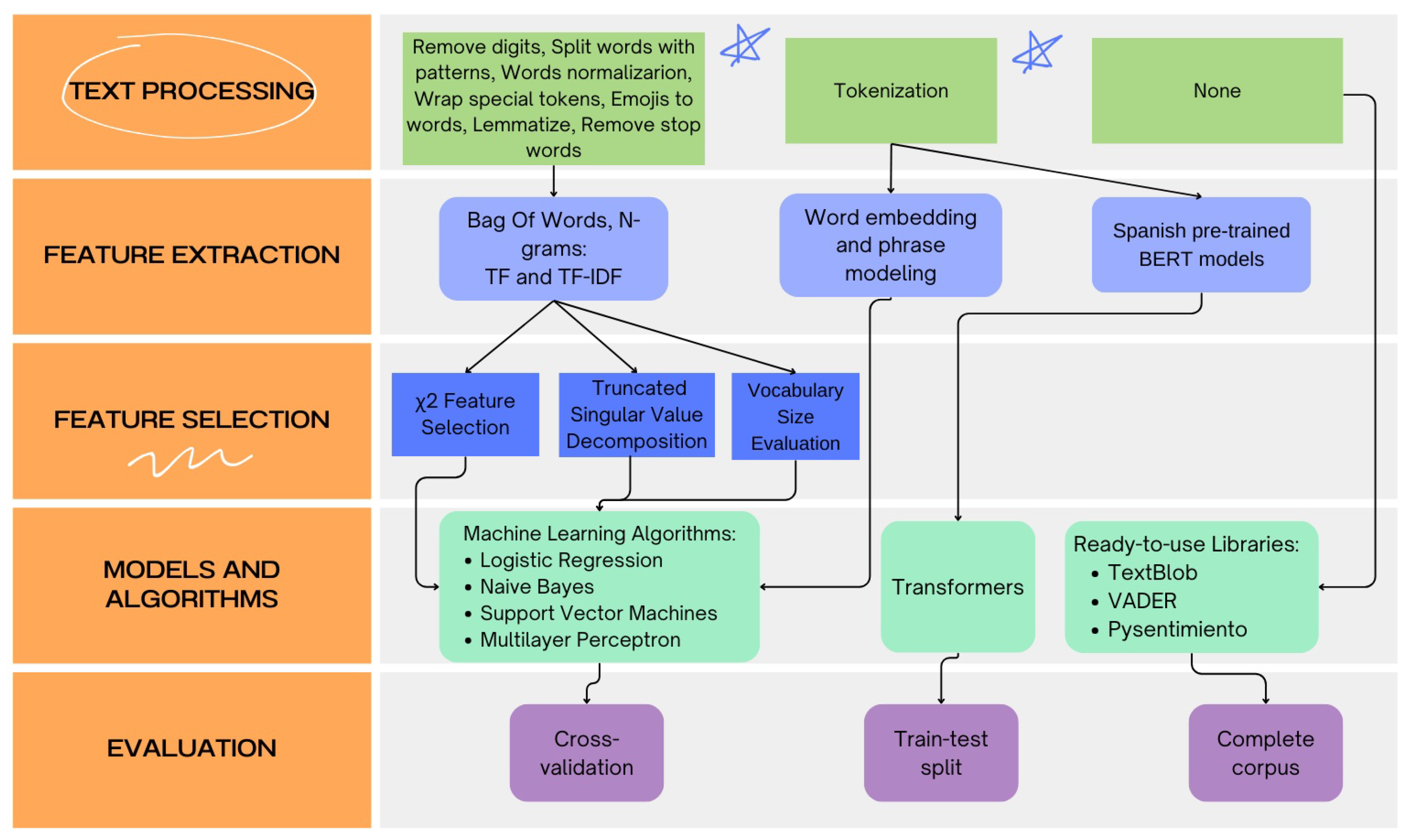
Figure 1.
Sentiment analysis experimentation workflow.
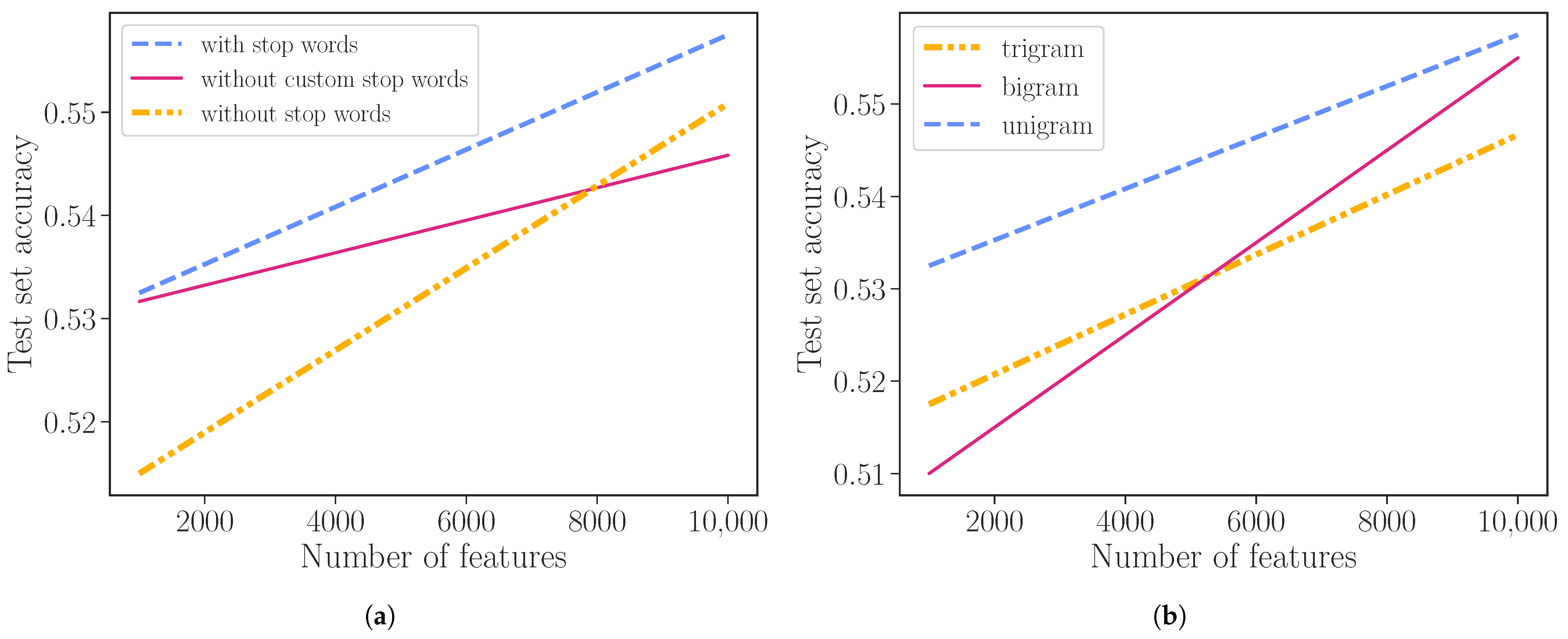
Figure 2.
Test Accuracy for different number of features. (a) Without vs with stopwords using unigrams. (b) n-gram test results. We tested .
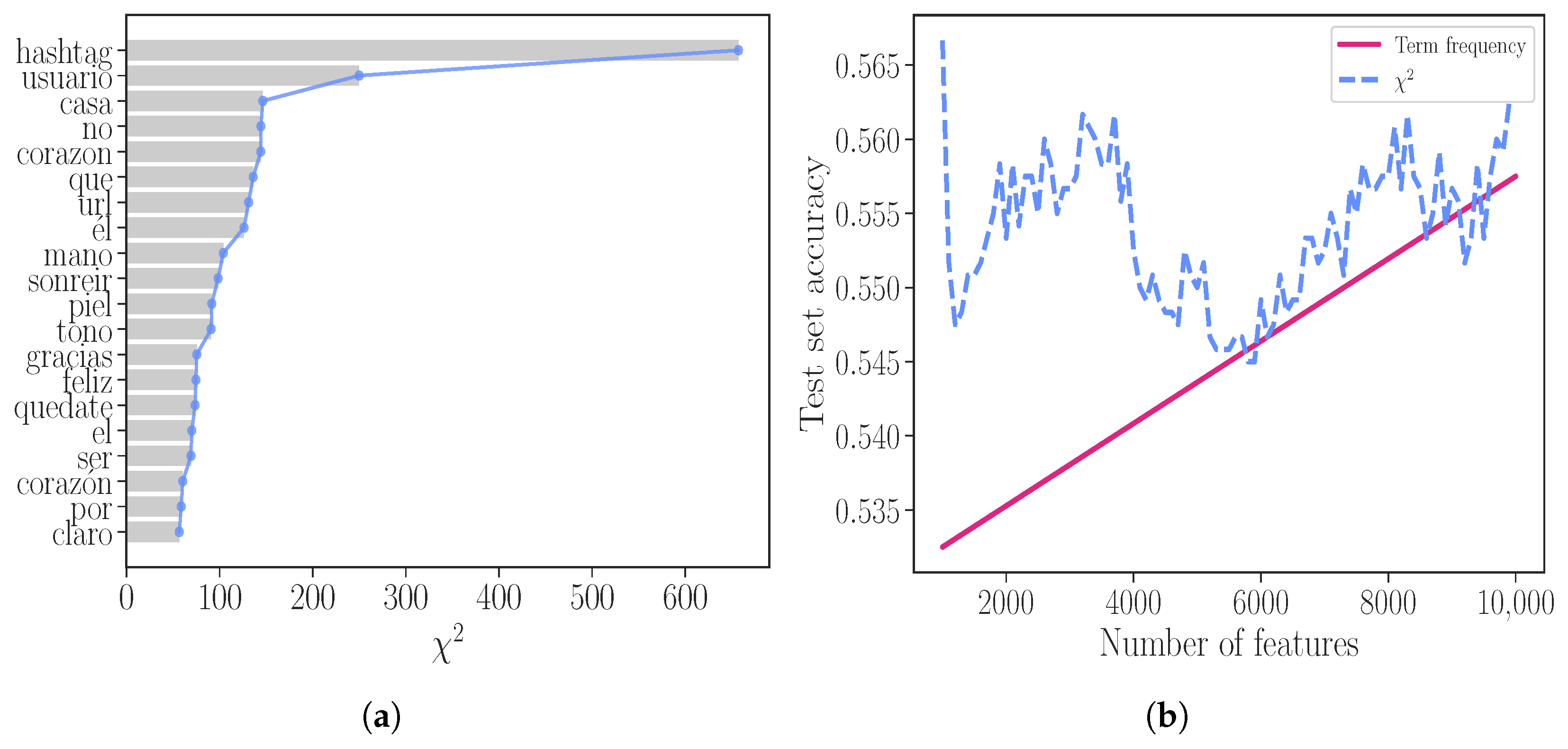
Figure 3.
(a) Most significant words given by and (b) accuracy on the test set for the different number of features. We show results for the term frequency vector reduced by the term frequency (solid line) and the (dashed line).
Figure 4.
Explained variance for n components.
Table 1.
Lexicon used to filter the COVID-19 related tweets for the corpus creation.
| VARIANTS COVID | SYMPTOMS |
|---|
| COVID-19 | me dio diarrea |
| coronavirus | dolor de cabeza agudo |
| Covid-19 | cuerpo cortado |
| Coronavirus | fiebre (leve) |
| Covid19 | tos (seca) |
| Covid | dolor de garganta |
| lo del contagio | altas tamperaturas |
| esta pandemia | |
| Corona Virus | |
| el virus | |
| HASHTAGS | HASHTAGS |
| #AbrahamSealaverga | #Covid19 |
| #AburridoEnCasa | #covidmexico |
| #AislamientoSocial | #CuarentenaCoronavirus |
| #BastaDeFakeNews | #CuidaALosTuyos |
| #carroñavirus | #CuidemosALosMayoresYPequeños |
| #CODVID19 | #EnCuarentena |
| #ConferenciaCovid19 | #MeQuedoEnHome |
| #ConLaFuerzaDeLosProtocolosSI | #NoSonVacaciones |
| #Coronavirus | #QuedateEnCasa |
| #CoronavirusMx | #QuédateEnTuCasa |
| #coronaviruspeleishon | #COVID19mexico |
| #COVID19mx | #CuandoEstoSeAcabe |
| #Cuarentena | #cuarentenamexico |
| #CuidaALosDemas | #CuidarnosEsTareaDeTodos |
| #Cuidate | #CulturaEnCasa |
| #encasa | #Enfermera |
| #MeQuedoEnCasa | #México |
| #NeumoniaAtipica | #QuedarseEnCasa |
| #quédate | #QuédateEnCasaUnMesMas |
| #QuedateEnLaCasa | #QuedateEnTuCasaCarajo |
| #quedateentuputacasaalaverga | #QuedenseEnCasa |
| #QuePorMiNoQuede | #sabadodecuarentena |
| #SaltilloQuédateEnCasa | #SeFuerteMexico |
| #SiTeSalesTeMueres | #StayAtHome |
| #StayAtHomeAndStaySafe | #Super |
| #SusanaDistancia | #teamwork |
| #TecuidasTúNosCuidamosTodos | #TipsDeCuarentena |
| #ÚltimaHora | #UltimaOportunidad |
| #YaBastaDeFakeNews | #yolecreoagattel |
| #YoMeQuedoEnCASA | |
Table 2.
Agreement score by the annotators of the classification of sentiments without a guide.
| Annotator Pair | A&B |
|---|
| Percent of agreement | 41% |
| Cohen’s score | 0.1785 |
Table 3.
Agreement scores by each pair of annotators of the classification with the guide.
| Annotator Pair | 1&2 | 2&3 | 1&3 |
|---|
| Percent of agreement | 61% | 70% | 62% |
| Cohen’s score | 0.3945 | 0.5547 | 0.3716 |
Table 4.
General statistics computed from word counts on each tweet.
| | Positive Tag | Negative Tag | Neutral Tag |
|---|
| Average number of words per tweet | 22.85 | 26.39 | 20.97 |
| Standard Deviation | 12.69 | 15.46 | 13.59 |
| Variance | 161.14 | 239.02 | 184.65 |
| Minimum number of words in a tweet | 3 | 3 | 3 |
| Maximum number of words in a tweet | 59 | 339 | 88 |
| Total number of words | 25,729 | 48,398 | 38,580 |
| Tweets count | 1126 | 1834 | 1840 |
Table 7.
Sorted features with smallest and largest Tf-Idf values.
| Tf-Idf Values | Features |
|---|
| Smallest | ‘buen lunes’, ‘app’, ‘inicio semana’, ‘inmediato’, ‘oms’, ‘periodico hoy’ |
| ‘alto contagio’, ‘ganar seguidor’, ‘calidad’, ‘amlolujo’ |
| Largest | ‘financiero’, ‘muerte covid’, ‘lugar’, ‘movil’, ‘movilidad’, ‘dar positivo’ |
| ‘lopez’, ‘muerte’, ‘cuidarte profesional’, ‘gracia’ |
Table 8.
Phrase detection tokens yield by each model.
| | Phrase Detection |
|---|
| Unigram | [‘@usuario’, ‘por’, ‘su’, ‘trabajo’, ‘no’, ‘es’, ‘justo’, |
| | ‘para’, ‘los’, ‘demas’, ‘quedate’, ‘en’, ‘casa’] |
| Bigram | [’@usuario’, ‘por’, ‘su trabajo’, ‘no es’, |
| | ‘justo’, ‘para’, ‘los’, ‘demas’, ‘quedate’, ‘en casa’] |
| Trigram | [’@usuario’, ‘por’, ‘su’, ‘trabajo’, ‘no es |
| | justo’, ‘para’, ‘los’, ‘demas’, ‘quedate en casa’] |
Table 9.
TextBlob outputs for different statements in Spanish.
| Input | ‘polarity’ | ‘subjectivity’ |
|---|
| Este teléfono tiene una pantalla de excelente resolución, además es muy rápido | 0.63 | 0.89 |
| Este teléfono tiene una pantalla de alta resolución, además es rápido | 0.18 | 0.57 |
| Este telefono es lo máximo, lo adoro <3 :D | 1.0 | 1.0 |
| Este telefono no me gusta :( | −0.75 | 1.0 |
Table 10.
Vader outputs for different statements (in Spanish).
| Input | ‘neg’ | ‘neu’ | ‘pos’ | ‘compound’ |
|---|
| hoy es un pésimo día | 0.779 | 0.221 | 0.0 | −0.5461 |
| hoy es un mal día | 0.646 | 0.354 | 0.0 | −0.7424 |
| hoy es un día cualquiera | 0.123 | 0.637 | 0.24 | 0.231 |
| hoy es un gran día | 0.0 | 0.408 | 0.592 | 0.5404 |
| hoy es un excelente día | 0.0 | 0.294 | 0.706 | 0.8633 |
Table 11.
Distribution of labels in the train and test partitions.
| (Seed = 37) | Negative | Neutral | Positive |
|---|
| Train | 33.642% | 44.934% | 21.422% |
| Test | 34.899% | 44.380% | 20.713% |
Table 12.
Accuracy for n components.
| n_components | Accuracy |
|---|
| 1000 | 63.12% |
| 1500 | 64.79% |
| 2000 | 65.76% |
| 2500 | 65.51% |
| 3000 | 64.83% |
Table 13.
Test accuracy for Doc2Vec models. The best result is highlighted in bold.
| | 1-Gram | 2-Gram | 3-Gram | Best |
|---|
| DBOW | 60.642% | 59.934% | 60.422% | 60.642% |
| DMC | 56.893% | 54.387% | 55.713% | 56.893% |
| DMM | 59.641% | 58.935% | 57.253% | 59.641% |
|
DBOW+DMC
| 61.927% | 61.234% | 62.422% | 62.422% |
|
DBOW+DMM
| 63.185% | 62.617% | 63.373% | 63.373% |
Table 14.
Optimal hyperparameters settings selected for each model based on th optimization of accuracy through grid-search and cross-validation.
| GridSearchCV (CV = 10) |
|---|
| Model | Hyperparameters Tested | Optimal Value |
Logistic
Regression | | |
Multinomial
Naive
Bayes | | |
| SVM | | |
Multilayer
Perceptron | | |
Table 15.
Results of the obtained by training the classification algorithms on the three feature sets. The best result is highlighted in bold.
| Unconstrained BoW |
|---|
| | KNN | SVM | MNB | Logistic | MLP |
| Accuracy | 59.75% | 62.31% | 62.03% | 64.26% | 63.51% |
| Precision | 60.08% | 62.25% | 63.24% | 64.39% | 63.92% |
| Recall | 59.76% | 62.31% | 62.03% | 64.25% | 63.51% |
| F1-score | 58.78% | 61.96% | 60.78% | 63.61% | 62.59% |
| BoW reduced with SVD |
| | KNN | SVM | MNB | Logistic | MLP |
| Accuracy | 60.88% | 64.98% | 64.19% | 67.12% | 68.84% |
| Precision | 61.40% | 64.91% | 62.27% | 66.91% | 67.25% |
| Recall | 60.88% | 64.98% | 64.19% | 67.12% | 68.84% |
| F1-score | 59.92% | 64.02% | 62.98% | 66.24% | 67.90% |
| Doc2Vec with DBOW+DMM |
| | KNN | SVM | MNB | Logistic | MLP |
| Accuracy | 56.47% | 62.56% | 62.96% | 63.68% | 64.31% |
| Precision | 54.76% | 63.81% | 63.54% | 61.94% | 60.81% |
| Recall | 56.47% | 62.56% | 62.96% | 63.68% | 62.31% |
| F1-score | 42.93% | 57.59% | 63.88% | 61.55% | 62.11% |
Table 16.
Results obtained by the sentiment analysis libraries. The best result is highlighted in bold.
| | TextBlob | Nltk Vader | Pysentimiento |
|---|
| accuracy | 51.23% | 58.07% | 68.89% |
| precision | 55.45% | 58.60% | 72.20% |
| recall | 51.23% | 57.19% | 52.81% |
| F1-score | 52.92% | 56.42% | 60.38% |
Table 17.
Classification results of the Spanish BERT models. The best result is highlighted in bold.
| | BETO-Uncased | roBERTa-Sentiment | BerTin-Base |
|---|
| training set accuracy | 96.20% | 97.54% | 96.91% |
| validation set accuracy | 73.26% | 71.88% | 72.14% |
| validation loss | 0.3945 | 0.2847 | 0.2141 |
Table 18.
Results of an increasing number of epochs using BETO. The best result is highlighted in bold.
| Epoch | Train Set Accuracy | Test Set Accuracy | Validation Loss |
|---|
| 3 | 92.89% | 70.33% | 0.4554 |
| 5 | 96.20% | 73.26% | 0.3945 |
| 10 | 97.12% | 72.76% | 0.3161 |
Table 19.
Summary of the performance evaluated based on the accuracy of different sentiment analysis models on the SENT-COVID corpus. The best result is highlighted in bold.
| Model | Accuracy |
|---|
| TextBlob | 51.23% |
| Nltk Vader | 58.07% |
| Pysentimiento | 68.89% |
| SVM | 64.89% |
| Naive Bayes | 62.22% |
| Logistic Regression | 67.12% |
| MLP | 68.84% |
| BETO-uncased | 73.26% |
| roBERTa-sentiment | 71.88% |
| BerTin-base | 72.14 % |
| Disclaimer/Publisher’s Note: The statements, opinions and data contained in all publications are solely those of the individual author(s) and contributor(s) and not of MDPI and/or the editor(s). MDPI and/or the editor(s) disclaim responsibility for any injury to people or property resulting from any ideas, methods, instructions or products referred to in the content. |
© 2024 by the authors. Licensee MDPI, Basel, Switzerland. This article is an open access article distributed under the terms and conditions of the Creative Commons Attribution (CC BY) license (https://creativecommons.org/licenses/by/4.0/).


 ,
, 


 #Coahuila #Mexico 😥
 ALERTA alto contagio en los mochis