Article

Detecting Transitions in Manual Tasks from Wearables: An Unsupervised Labeling Approach †

by
Sebastian Böttcher
1,*,
Philipp M. Scholl
2 and
Kristof Van Laerhoven
3
1
Epilepsy Center, Department of Neurosurgery, Medical Center—University of Freiburg, 79106 Freiburg, Germany
2
Embedded Systems Group, Computer Science Institute, University of Freiburg, 79110 Freiburg, Germany
3
Ubiquitous Computing Group, Faculty of Science and Technology, University of Siegen, 57076 Siegen, Germany
*
Author to whom correspondence should be addressed.
This article is an expanded version of the original conference paper [1] and includes a new, in-depth review of related work, as well as additional classification results for some supervised methods on the same datasets and a performance comparison of all methods.
Informatics 2018, 5(2), 16; https://doi.org/10.3390/informatics5020016
Submission received: 28 February 2018 / Revised: 23 March 2018 / Accepted: 26 March 2018 / Published: 29 March 2018
(This article belongs to the Special Issue Sensor-Based Activity Recognition and Interaction)

Abstract

:
Authoring protocols for manual tasks such as following recipes, manufacturing processes or laboratory experiments requires significant effort. This paper presents a system that estimates individual procedure transitions from the user’s physical movement and gestures recorded with inertial motion sensors. Combined with egocentric or external video recordings, this facilitates efficient review and annotation of video databases. We investigate different clustering algorithms on wearable inertial sensor data recorded on par with video data, to automatically create transition marks between task steps. The goal is to match these marks to the transitions given in a description of the workflow, thus creating navigation cues to browse video repositories of manual work. To evaluate the performance of unsupervised algorithms, the automatically-generated marks are compared to human expert-created labels on two publicly-available datasets. Additionally, we tested the approach on a novel dataset in a manufacturing lab environment, describing an existing sequential manufacturing process. The results from selected clustering methods are also compared to some supervised methods.

Graphical Abstract

1. Introduction

Identifying steps of manual work, either in real-time or off-line recordings, can support or guide the worker with just-in-time information in the context of the current work step. A possible approach to this problem of step identification, followed in this paper, is to detect transitions between steps instead of distinguishing what is actually executed. While this does limit possible applications, since it will not allow one to query for particular activities, it does provide marks in concurrently recorded video material to provide a first set of navigation cues for later refinement. Possible application areas include laboratory experiments, preparing food, manual labor or any kind of repetitive activities that follow a (semi-)fixed procedure. The order and/or number of steps in the process may be known beforehand, such that a classifier must only detect transitions from one state to another. However, instead of using classifiers to exactly identify steps executed at a particular point in time, as is usually done, we argue that it is beneficial to only target the detection of the duration of each step, thereby significantly simplifying the problem. This approach obviates the need for labeled data.
We aim at an automatic detection of such transitions based on inertial data recorded on the human body, with simultaneous and synchronized video recordings for visual inspection afterwards. Point-of-view video recordings of manual processes have become easier to record with recent commercial devices, but tend to be hard to browse, both due to their length and because interesting marks in those videos are hard to find. A clustering of the body motion provides here a first index into such repositories, e.g., being able to skip sequences where there is little or no movement, or quickly jumping from one point of interest to another. Furthermore, the paper presents an extended survey of literature in the field of Activity Recognition (AR) and its various sub-domains with focus on wearable motion classification, aiming to give an overview of the field in general and established work therein by compiling popular methods used in both unsupervised and supervised AR, as well as showing past work in process recognition.
Figure 1 shows an example of the clustering approach applied to a recording of wrist motion and documentation video data of a DNA extraction experiment. Blue vertical bars indicate transitions between clusters in the data, found via k-means clustering. The graph also shows the ground truth transitions, extracted by visual inspection, in different background colors. Video stills from the recording show the process at various points in time. The whole video can thus efficiently be traversed by jumping from one transition mark to another. In an extended consideration of the problem, the recognition of step transitions should be possible regardless of the scenario or data provided, motivating the use of unsupervised methods beyond their obvious advantage of not having to manually label training data.
The remainder of this paper is structured as follows: First, a survey of related work is compiled to situate the paper amongst the current state of the art. Following this, we present the system design, which is capable of efficiently solving the problem of separating possible process steps. The system is then applied to three real-world datasets that include video and inertial data, including one new and thus far unpublished one. An evaluation is then performed on these to gather recall performance for different approaches, unsupervised and supervised as a comparison. In the last sections, the experiments’ results are discussed in-depth, and a summary of contributions, conclusions and a short outlook are given.

2. Activity Recognition and Related Work

2.1. AR with Inertial Sensors

Inertial sensors as used in this work comprise a commonly-used and widely-accepted method of sensing human motion for AR. Inertial Measurement Units (IMUs) provide acceleration, angular velocity and magnetic field strength measurements via an integrated accelerometer, gyroscope and magnetometer, respectively. They can for example be applied to ambulatory [2,3] or daily life [4,5] gesture recognition among other scenarios. Often, accelerometer data are sufficient to recognize basic human motions, and additionally using gyroscope and magnetometer data can introduce higher computational cost [6]. However, full IMU data are preferred in more complicated scenarios or when dealing with possible sensor displacement [3]. It is also absolutely essential in contexts where rotation in addition to linear movement are of interest [7], e.g., when tracking hand or wrist movements [8]. IMUs are easily available as standalone sensors and nowadays built into most consumer wearables like smartphones or smartwatches. In [9,10], for example, a smartphone is used to record IMU data for use in daily life activity recognition, and [11] investigate the feasibility of smartwatches for hand and finger gesture recognition. The works in [4,12,13], on the other hand, use a custom-made sensor platform for AR, which additionally gives the opportunity to use multiple sensor platforms in a small network to gather data from various body positions at the same time, as in [14,15]. Data collected from IMUs furthermore lend themselves to the extraction of a multitude of different features, most prominently in the time or frequency domain [16]. Raw data are also often used [14], particularly in real-time applications. With respect to classification of motion gestures with inertial data, both supervised and unsupervised (e.g., [17,18]) methods have been used, with unsupervised methods gaining popularity in recent years. Inertial sensors in wrist-worn devices like smartwatches are used in a plethora of other scenarios, including, but by far not limited to smoking detection and tracking [19,20], posture tracking [21] and workspace interaction support [22].

2.2. AR via Image Processing

In addition to inertial sensor data, the datasets used in this paper all include the additional component of video recordings of the subjects during their actions. Some of these video recordings are from stationary cameras overlooking the relevant experimentation area, and some are from body-cameras showing an ego-centric perspective from the participants’ view. There are several works proposing recognizing human activities from images or video. A popular approach is using depth-enhanced (RGB-D) video data to construct a skeleton representation of the human body and estimate activities based on the calculated poses of the participant [23,24,25]. While this is a valid approach in general, we do not use the video data in our recognition system, not only because no depth data are provided in the datasets, but because it would add significant complexity to our otherwise deliberately simple approach to recognizing steps in a process.

2.3. Unsupervised AR: Clustering

In unsupervised learning, the raw data are completely unlabeled. Rather than using labeled data to build models that match data to certain categories, unsupervised “classifiers” are discriminative and aim to detect distinct structure in the data, often taking advantage of the fact that the feature space is clustered with respect to different activities. The immediate disadvantage of this approach is however that data are matched not to meaningful categories, but oftentimes to an identifying cluster index or similar key. Different clustering methods and metrics exist, but most can be reduced to the concept of “if two data points are close to each other, according to some metric, they belong to the same cluster”. While most clustering methods are considered unsupervised learning methods, some supervised and semi-supervised methods have been presented, as well [26,27]. Algorithms thus produce for each given sample a cluster index, usually an integer, where samples with the same index belong to the same detected cluster and thus are classified as related. In activity recognition, while most raw data may not be easily clustered, samples in feature space often show distinct structure. The choice of features can thus be the most important aspect of a successful clustering, resulting in an informative and cluster-able feature space with respect to the sought property, or useless data. Some clustering algorithms also give an opportunity to specify the expected number of clusters, therein limiting the produced number of cluster indices to a maximum.
Partition clustering is arguably the most basic of the clustering variants [28,29,30]. It poses a common baseline in unsupervised learning and is usually the first place to go for researchers to test their data for clusters. Even though many other clustering algorithms have been developed since the development of k-means in the 1950s, it is still a widely-used method for finding structure in data [17,31,32,33,34].
Whereas partition clustering (k-means) assigns data points by iteratively minimizing the sum-of-squares error for each cluster, hierarchical clustering algorithms impose a hierarchical structure on the data based on some relation between data points. This can be done in either a bottom-up manner where each data point starts in its own cluster and the most similar clusters are merged (agglomerative clustering), or in a top-down manner where all data points start in the same cluster, which is then recursively divided (divisive clustering) [31,35]. In activity recognition, hierarchical clustering seems to be somewhat unpopular and used only as an extension to other more powerful methods [36,37].
Density-based clustering considers areas with a high density of data points as clusters, while low density areas represent the partitioning, i.e., the margin between clusters. As such, density-based algorithms are robust against outliers, which are regarded as part of the sparse areas between clusters and thus ignored. Another important property of density-based algorithms is that clusters can be of arbitrary shape, while most other methods have some underlying requirement on the shape of the data. A popular example of density-based clustering is the DBSCAN algorithm [38,39,40].
Mixture models in general are a way of representing subgroups in a set of observations without the need for each observation to specify their respective group. Gaussian Mixture Models (GMM) assume the data to be distributed from a certain number of Gaussian distributions. It can therefore be seen as a generalization of the k-means algorithm, with the cluster covariance as an additional variable. Expectation maximization is employed to fit the mixture of Gaussians on the data [41]. Furthermore, variants that assume an infinite number of Gaussian components have been proposed [42]. GMMs have been used for example to classify multiple-limb motion using myoelectric (EMG) signals [43] or recognizing human motion from RGB-D camera data [25].

2.4. Unsupervised AR: Motif Discovery

Motif discovery is a different approach to unsupervised learning, which is not directly related to clustering, and can alternatively also be applied as a supervised method. In motif discovery, which has its origins in DNA sequencing research [44,45], time series data are broken down into a set of reoccurring instances, i.e., motifs, by symbolizing the series and then searching for sets of connected symbols. These motifs, sometimes also called frequent patterns or sequences [46,47], can then be applied in several kinds of classification methods. Minnen et al. [48] uses motif discovery in a three-step system that first searches for a set of seed motifs, refines these and then trains an HMM for each of the motifs. The system is evaluated on an accelerometer and gyroscope dataset, using the raw data as input for the algorithm. Vahdatpour et al. [49] extends the probabilistic motif discovery [45] by the ability to process multidimensional time series. They propose a two-step algorithm that first discovers motifs on single dimensions and then applies graph clustering to determine correlations between motifs from different dimensions. Peng et al. [18] proposes a system that uses language-based grammar induction to detect low-level movements and intelligently group them into high-level activities. The works in [12,50] propose a supervised dense motif discovery approach that classifies actions through abstraction of sensor data into symbol strings. Raw accelerometer data are first linearized into segments, which are then pairwise discretized into symbols. A suffix tree algorithm then searches for reoccurring symbol substrings in a fixed window for each activity. To avoid misclassification, the set of substrings for a target activity is then trimmed by those substrings that also occur in the remaining data. From the new subset, a bag-of-words classifier is modeled per activity.

2.5. Supervised AR

The origins of activity recognition are largely based in supervised learning, being more accessible for research purposes at the time and yielding good results in most scenarios. Thus, there have been many different algorithms and variations thereof proposed over the years, and most are not specific to activity recognition, but have their source in other fields of machine learning and data analysis. As opposed to unsupervised learning, supervised methods make use of some kind of ground truth labeling that is applied to the data to generate models that can classify new unlabeled data. In general, models are thus trained with a certain set of data points that were labeled beforehand, often by hand by some expert on the subject matter of the application. As such, supervised methods are usually preceded by a significant human overhead. As with unsupervised learning, the choice of features can be significant for supervised methods, as well. Especially for motion data in activity recognition, there is an abundance of features to choose from, such that an additional step of feature selection is often necessary to reduce the dimensionality of the training input data. This section will present the most widely-used supervised methods and some example applications in AR-related literature.
Decision tree classifiers are used in several works with favorable results. They are a graph-based method using a tree to model decisions in a classification problem, i.e., branches represent different attribute values and leaves represent classes. In its simplest form, attributes are tested, and depending on their values, a different path in the tree is chosen, until a class is reached. The C4.5 decision tree algorithm was originally proposed in 1993 as an extension of the ID3 algorithm from 1986 [51,52]. In the top 10 data mining algorithms, C4.5 decision trees placed at rank one [53], and they have been used in some AR works with favorable results [54,55]. An extension to the decision tree method are “random forests”, first proposed in 1995 and later revised in 2001 [56,57]. It is an ‘ensemble’ method, combining many randomly-generated single decision trees into a ‘forest’, classifying via majority vote of the trees. It rectifies a common problem single decision trees have, that is overfitting the data used for training. While a decision tree may perform very well on the training data, it might perform poorly on new data it has not seen before since it has also modeled noise in the training data. Training multiple trees on random subsets of the data smooths out this high variance in a way.
Another popular classification method in supervised learning is the k-nearest neighbors algorithm [58]. It is a supervised clustering method that takes advantage of the fact that data samples, or features thereof, are often clustered with respect to their activity class. K-NN classifies instances via the majority vote of the k-nearest training data samples, measured by some specified distance measure. Since the method does not require a complex model to be trained, k-NN classifiers only save the raw training data for classification purposes. Methods like this are also called ‘lazy learners’.
Support Vector Machine (SVM) [59] is a popular non-probabilistic classification method for binary problems. It is based on the principle of dividing data with a hyperplane into two classes while keeping the margin between the two classes and the hyperplane as large as possible. As such, it is a linear classifier; however, by moving the samples into a much higher dimension and using the kernel trick on the hyperplane, the method can also produce a non-linear classifier. SVMs can be applied to multiclass problems, as well by reducing the problem to multiple binary classifications, for example via the common one-versus-one or one-versus-all methods. Due to their versatility, SVMs have been used in many activity recognition works, for example in [60,61].
Linear Discriminant Analysis (LDA) and Quadratic Discriminant Analysis (QDA) [62] are classical methods to find a separation surface in a given feature space, either linear or quadratic in nature, respectively. While they are often used as linear and quadratic classifiers, LDA specifically can also be used as a tool for supervised dimensionality reduction in multiclass problems. Neither method has any hyperparameters to choose and can be used on binary, as well as multiclass problems, and they have been used successfully in AR-related work [2,63].
Artificial neural networks [64] are becoming a more popular method for modeling an activity classifier in recent years [65]. They process usually a very large amount of training data to approximate decision functions for a recognition model. Neural networks are large networks of neuron-like nodes, typically distributed over multiple layers, which are interconnected. Each node may have an algorithm or simple function that processes the inputs coming from previous nodes into outputs sent to following nodes, e.g., the sum of all inputs must reach a certain threshold to trigger an output. An example of this is the Multilayer Perceptron (MLP), which is such a network of artificial neurons with arbitrary non-linear activation functions. The work in [2] uses perceptron-based ANNs in a two-step recognition system The work in [9] uses an MLP as one of six different classifiers they test using accelerometer and gyroscope data recorded from a mobile phone.

2.6. Process Recognition
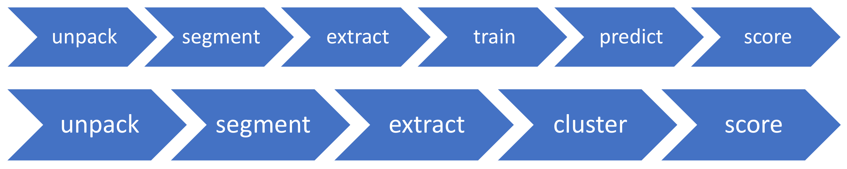
Detecting process steps to guide users through a workflow or for providing structured post hoc recordings was attempted several times already. RFID tags for example have been successfully used to track the movement of manufacturing parts throughout a process workflow [66,67]. Another popular approach is to use cameras and motion-tracking algorithms [68,69], for example in factory or surveillance applications, to track activities. Recent work is even using projectors to augment a user’s workflow in a process [70] to guide the users. A different environment is the kitchen where meal preparation could be of interest to health monitoring [71]. However, most aligned with the idea of this paper is the GlaciAR system [72], an authoring system for point-of-view videos based on object detection. We however employ wrist motion to detect significant steps. Another example is the wet lab support system proposed in [73], which is able to automatically document an experiment in a laboratory with a known protocol and wrist motion.

3. System Design

Since the activity recognition pipeline provides a multitude of tunable parameters that can greatly influence the outcome of the clustering and respectively the quality of automated indexing of video recordings, we propose a hyper-parameter evaluation approach in which test recordings are used to find a best parameter combination for unsupervised transition detection. In order to easily and efficiently process large numbers of parameter combinations, a lightweight tool geared towards parallel processing is needed [74]. It is implemented as a Unix command line utility, which provides several largely independent modules that can be employed by themselves, or subsequently linked in an efficient manner to form an activity recognition pipeline. This pipeline, shown in Figure 2, is thus the basis of our system: It processes the data source (unpack, segment), extracts features from each data segment (extract) and applies the chosen learning (train + predict) or clustering (cluster) methods. The output of these methods is then prepared for evaluation (score), which finally produces the pipeline results.
For the unsupervised methods, the experiments presented in the next section use the k-means clustering, agglomerative clustering and Gaussian Mixture Model (GMM) algorithms, all of which are implemented in scikit-learn. As we would like to compare the clustering performance to traditional supervised methods, we also employ the SVM, random forest, LDA and QDA methods, all implemented in scikit-learn. Refer to Section 2, which compiles a comprehensive list of algorithms including these and further provides in-depth descriptions of each method.
Classification with real-world data is not perfect, and noise in the classification output is a common occurrence in activity recognition. In most AR applications, this does not largely hinder the recognition of actions. However, in our scenario of unsupervised process step recognition, the clustering output has to be filtered to robustly detect transitions between states. We use a hysteresis filter to smooth the output and thus prevent false state transitions when multiple immediately concurrent samples are classified into different clusters. The filter works in that it only changes its output when a certain number of input samples in the future is the same as the one it is currently regarding.

4. Experimental Setup and Evaluation

To evaluate and compare the performance of the different clustering methods, we carried out an evaluation of three different datasets from independent sources. All three datasets include labeled human motion data, along with some form of video evidence as extra documentation.
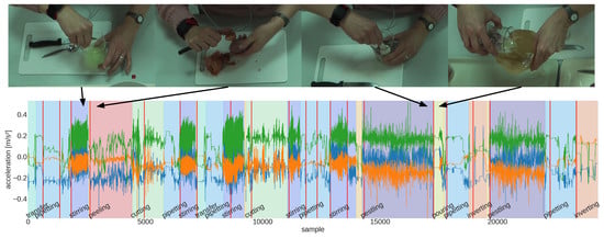
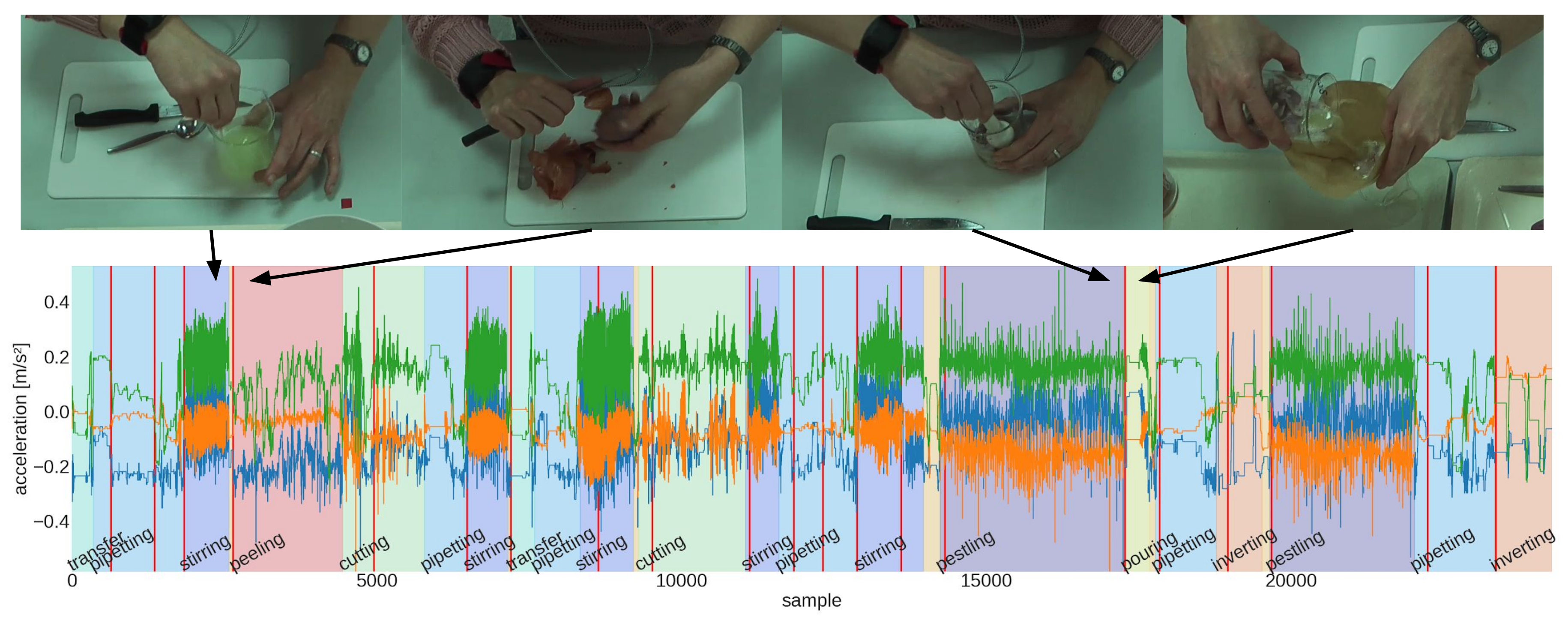
  • The DNA Extraction [73] dataset has 13 recordings of a DNA extraction experiments performed in a biological laboratory setting. Motion data from a single wrist accelerometer at 50 Hz are combined with videos from a fixed camera above the experimentation area. Experiments include 9 process steps, which may occur multiple times in one recording and in a semi-variable order.
  • CMU’s Kitchen-Brownies [75] dataset contains 9 recordings of participants preparing a simple cookie baking recipe. Motion data from two-arm and two-leg IMUs were recorded at 62 Hz . Video recordings from multiple angles, including a head-mounted camera, are included, as well. In total, the recipes consist of 29 variable actions.
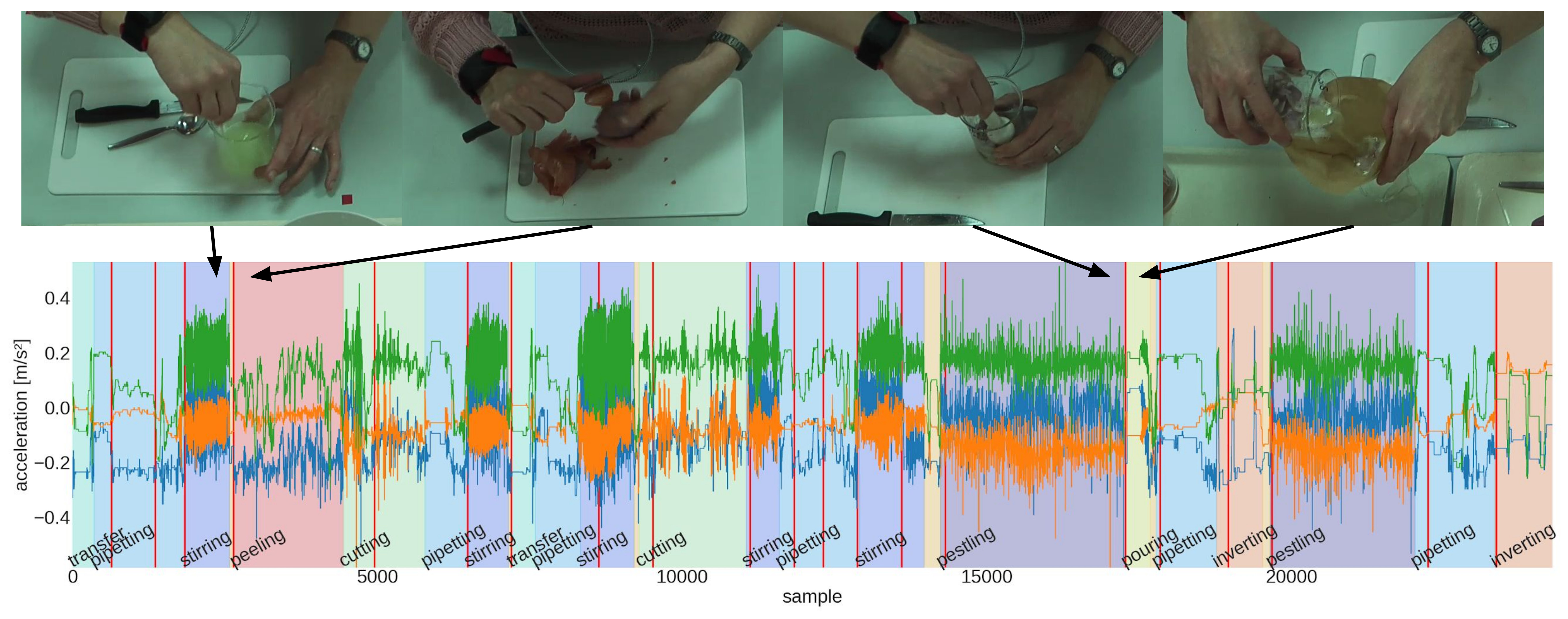
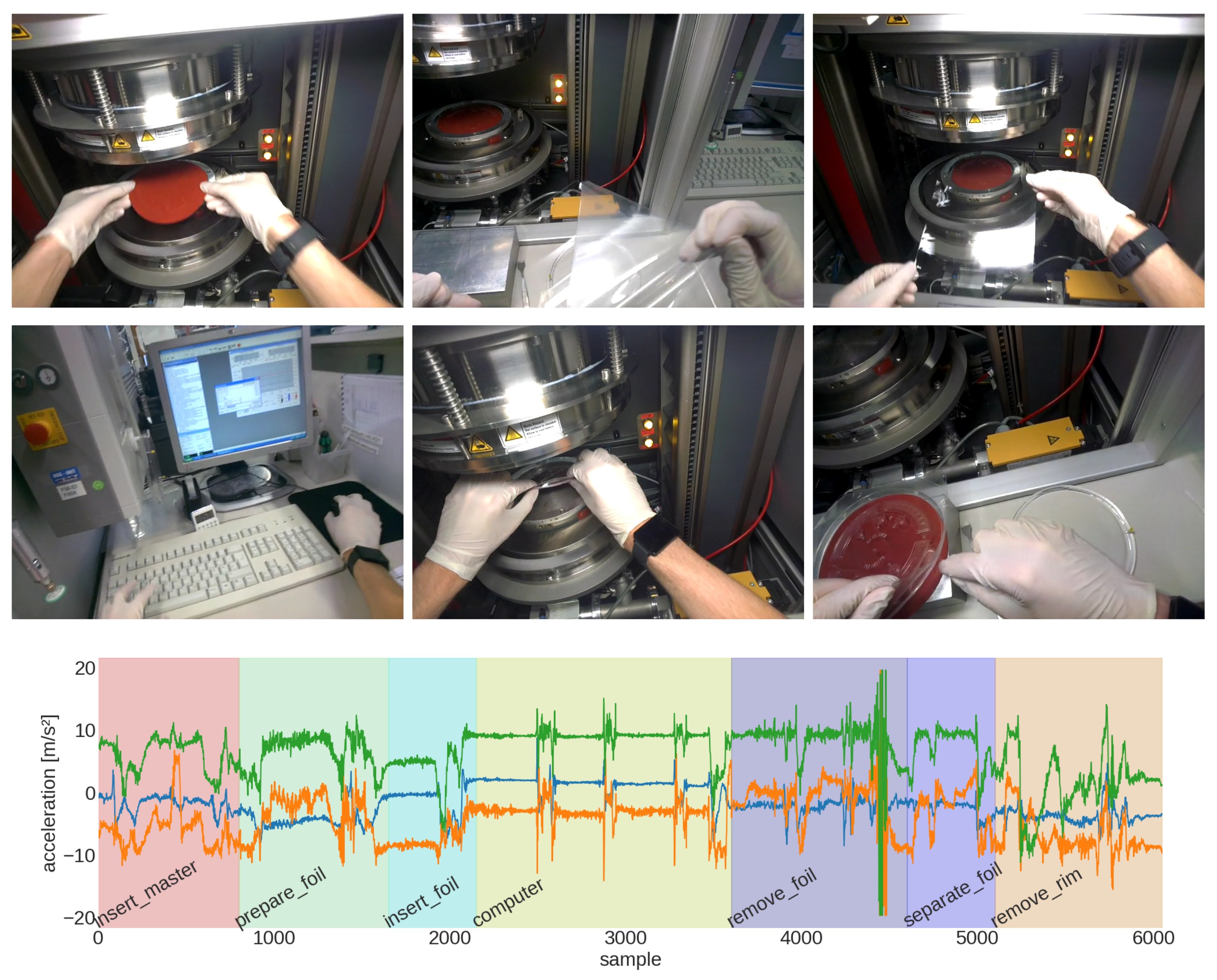
  • The Prototype Thermoforming dataset was recorded by ourselves and consists of two recordings of a thermoforming process of a microfluidic ‘lab-on-a-chip’ disk [76]. It combines IMU data at 50 Hz from a smartwatch and Google Glass and video recordings from the Google Glass. The datasets’ process contains 7 fixed process steps in a known order (see Figure 3).
While the sensor setups across all three datasets are somewhat heterogeneous, each dataset provides data from a unique scenario where linear processes are sequentially executed by the subjects. These heterogeneous sensor setups also provide a challenging setting for any evaluation across all datasets, which is described in more detail later.
The raw data from each dataset is preprocessed before they are forwarded to the clustering algorithms. First, the data are stripped of samples that are not or negatively labeled (e.g., labeled NULL), which may considerably clean noise from the input, depending on the dataset and individual recording. The data are then segmented by applying a sliding window of variable length, without overlaps between consecutive windows. For each segment, a number of features is extracted, specifically the mean and variance of the segment, in addition to the min-max range and the median.
After preprocessing and feature extraction, the clustering algorithms are applied to the feature data: k-means and agglomerative clustering along with Gaussian Mixture Models (GMM) are regarded for the experiments and furthermore compared to the supervised methods Random Forest (RF), Support Vector Machine (SVM) and Linear and Quadratic Discriminant Analysis (LDA/QDA). For k-means and agglomerative clustering, the results are evaluated per participant, since no actual training is necessary, and for the GMM clustering and the supervised methods, leave-one-participant-out cross-validation is performed.
To score the performance of clustering, the time-series data are clustered, and the resulting cluster edges are compared to the labeled ground truth. Cluster edges are regarded as process step transitions and, within a certain margin, are considered to be True Positives (TP) if they coincide with the transition of a ground truth label. If, however, a ground truth transition is not met by the clustering, a False Negative (FN) event is registered, and vice versa, a False Positive (FP) event is registered if a cluster edge happens with no corresponding ground truth transition (see Figure 4). In terms of event-wise evaluation, as proposed in [77], a true positive as described above can be considered an event match, i.e., a transition in the ground truth is matched by one in the cluster output. Likewise, a false negative can be regarded as an event deletion, and a false positive corresponds to an event insertion. However, the transition scoring approach results in a reduced scoring input set of only one sample per transition and also leads to no fragmented or merged events as described in [77], rendering that evaluation approach inapplicable. Event analysis diagrams are best applied to a full data series of ground truth and prediction labels, which is not the case here.
For supervised methods, the experiments are scored once by this transition scoring approach, which transforms the original multiclass problem into a binary one regarding only transition hits and misses, and once by the traditional multiclass scoring employing the full class label predictions given by the methods and compared to the ground truth. These two scoring approaches are indicated as “trans” and “multi” in Table 4 and Table 5.
Furthermore, we argue that false positives might in a real-world application not be as harmful as false negatives, since generating additional indices in an archived video file is not necessarily bad; missing a transitions however is. Hence, when scoring the experiments presented here, special attention is given to the recall measure, which provides a performance measure of how many of the ground truth transitions have a corresponding cluster edge, i.e., the amount of correctly-identified transitions.
To find the best parameter combination for unsupervised transition detection, a hyper-parameter approach is applied, in which each data recording is processed multiple times with different parameter combinations. The parameters that are varied per experiment run are the segmentation window length between 10 and 100 samples, the extracted feature with choices of mean, variance or an aggregated time feature, which combines mean, variance, range and median features, and the transition scoring margin mentioned above, between 1 and 5 samples. Each unique combination of these parameters is then applied to each combination of dataset recording, modality and algorithm as already described. Furthermore, the clustering methods provide a “number of clusters” parameter, which was also varied during the experiments, but is not included in the results and discussion, as we want to put specific focus on the pipeline parameters. The impact of this parameter on the scores proved to be negligible; the parameter was varied between 2 and 10, but there were high-scoring experiments with cluster number values on both ends of this range and between. This is unsurprising, since the transition scoring described above does not regard the cluster index, only the existence of a transition. For both the unsupervised and supervised methods, method parameters are not further varied than described here, and only the default scikit-learn settings are used.
Since there is high variation in the experiment parameters, each of the three datasets produces a large amount of scoring information. Different combinations of recording, sensor modalities, segmentation parameter, extracted feature and scoring parameter can yield tens of thousands of separate scores. To bring structure to the results, only the highest scoring parameter combinations are regarded for analysis. Table 1 shows results from the unsupervised experiments, specifically the top scoring parameters per dataset with their respective accuracy, recall, precision and F 1 -scores.
Furthermore, Table 2 and Table 3 show the supervised experiment results, again with the top scoring parameters per dataset with their respective accuracy, recall, precision and F 1 -scores. Table 2 lists the results of the transition scoring approach already described applied to the predictions made by the trained models on the test recordings. These scores thus present a direct comparison to the scores in Table 1 since the same scoring method was used. Table 3 on the other hand shows the results of only traditional scoring measures without the additional transition scoring approach. Thus, these scores represent a traditional multiclass classification on the datasets, with the respective pipeline parameters. Leave-one-participant-out cross-validation was used, i.e., the same experiment was run on each combination of one recording as the test set and the others as the training set. The mean of all cross-validation runs is then reported in the tables.
To get more information on a possible best parameter set for detecting process step transitions, the overall analysis of the scores is done in a three-step approach:
  • The results of each method across the three datasets with a recall score of ≥0.75 are intersected across the window, feature and margin parameters, since these are the pipeline parameters applicable to all methods and datasets. The intersection removes duplicates.
  • The experiment runs where the three parameters are the same as each parameter combination from the intersection are extracted, per method and dataset and again with recall ≥0.75, which gives three new tables per parameter combination (for each dataset).
  • The results are sorted and aggregated according to the recall scores of the DNA extraction dataset, since it provides a large number of individual recordings, simple modality and a relevant set of actions, which makes it the most useful dataset for measuring performance.
Table 4 compiles the highest scoring combinations of the resulting table and thus shows the performance of each listed method on all three datasets combined, and not just the individual scenarios, as in Table 1, Table 2 and Table 3.
As already mentioned in the beginning of this section, in all experiments scored so far, the input was significantly reduced by disregarding all samples labeled as NULL before preprocessing, thus removing possibly large sections of the input data where a subject was not performing actions belonging to the respective process. This reduction removes a large portion of the noise one would encounter when regarding real-life applications. To test the presented approach on data that are more representative of real-life scenarios, some of the already shown experiments were repeated on the DNA extraction dataset, this time without filtering NULL-labeled samples. The results of these additional experiments can be found in Table 5.
Figure 5 shows benchmarking data for the CMU Kitchen dataset. The processing time of the clustering, or training in the case of GMM, was logged for each run of the experiment with different parameters (top). Additionally, the runtime of each parallel job is logged, as well, showing the overhead that preprocessing and feature extraction create in the pipeline. Note that both graphs have a logarithmic y-axis scale. The recurring pattern of higher and lower processing times stems from the way the hyper-parameter approach iterates through possible combinations of parameters. Some combinations result in higher processing overhead, e.g., for GMM, the higher dimensionality when using all modalities at the same time results in very costly operations. Summarizing the benchmark results also for the other datasets, it can be seen that GMM performs on average much worse than k-means and agglomerative clustering only slightly better than k-means.

5. Discussion

Looking at the individual top scoring experiment runs (Table 1, Table 2 and Table 3), there is a parameter combination for each dataset and each detection method that can yield good recall scores for a robust detection of process steps. Comparing the best runs for the three datasets, there is however no clear winner for the method used. Furthermore, segmentation window lengths of around two seconds are set in all top scoring runs and thus seem to be the best choice for this parameter, as is the mean feature, which is sufficient in most cases to yield good results. Further considering results per individual dataset, the k-means and agglomerative clustering methods show the best results for each scenario. Within the considered scope of detecting transitions in linear processes, the simple, basic clustering methods seem to consistently perform better than more complicated approaches. Table 4 further shows that there are indeed parameter combinations that will yield good results in all of the regarded scenarios. Again, the k-means and agglomerative clustering methods generally achieve the highest scores. This result is most important with respect to our proposed problem, since it shows that these simple clustering approaches can perform well on detecting transitions in multiple different linear process scenarios.
Comparing the performance of unsupervised methods (Table 1) to those of supervised methods employing transition scoring (Table 2), the supervised methods have generally lower scores, reflecting the non-optimized method parameters, which have a larger effect on supervised methods than on simple clustering methods. In terms of performance over all datasets combined, a similar best parameter set is found for supervised methods as for the clustering methods. One difference is that for the random Forest method, the scoring margin set during the transition scoring process can consistently be lower than for all other methods. This means that the model output after smoothing is already sufficiently accurate with respect to transitions from one class to another. The supervised multiclass experiments (Table 3) show much lower scores than those with transition scoring of the same methods, demonstrating the reduction in problem complexity of that scoring method. Multiclass classification with non-optimized algorithm parameters on datasets of this kind will invariably yield lower scores, even if the pipeline parameters may be optimized. Even supervised methods without tunable hyperparameters (LDA/QDA) show significantly lower scores using this approach. The exceptionally low recall and precision scores for the CMU Kitchen multiclass supervised experiments are possibly in part due to the very high number of possible classes. Some error in the pipeline or the scoring may also be possibility. Overall, the low scores of supervised methods do not justify the added overhead on these methods of labeling the data for model training. However, the scores may be significantly better than is shown here if the algorithm parameters were additionally part of the hyper-parameter approach.

5.1. Limitations

In addition, several other factors need to be considered that may have influenced the results in a positive way. The applied smoothing step after clustering for example removes much uncertainty in the transitions, which may not be the case in comparable work. This factor is even further reinforced by the allowed margin of error applied when scoring the results. Furthermore, the datasets used in the experiments were specifically chosen for this application, i.e., they all provide clear-cut, distinct steps in a linear process. Dataset 3 also provides very little variance, in individual process composition, as well as in overall recordings, which explains the especially good results in this case.
Another factor is the complete disregard of NULL samples, i.e., samples where the original labeling provides no classification. These samples were removed from the input before clustering, giving the clustering algorithms a very clean input. Looking at Table 5, we can indeed see that the performance of experiments with the NULL samples still included in the input is consistently lower than their filtered counterparts, when compared to the scores in Table 1 and Table 3. Comparing recall scores, this is especially noticeable for the unsupervised methods, which perform 10 % worse when clustering on an input that still has NULL labels. This would result in a significant portion of the step transitions not being found in the output, while the input is noisier and considerably larger in length, exacerbating this negative result.
Noteworthy is also the fact that all three clustering algorithms used in the unsupervised experiments are in essence very similar, explaining the overall small variance in scores. GMMs can be seen as a generalization of the k-means method, where the cluster covariance is an additional variable. The implementation of agglomerative clustering used in the experiments applies Ward linkage, which minimizes the sum-of-squares error in each cluster, similar to the k-means algorithm.

6. Conclusions

The results show that even very basic clustering of the mean acceleration of the wrist can already robustly distinguish between single steps in a linear process. This is a rather surprising result, since usually much more elaborate methods need to be employed to provide good recognition results. However, our goal was not to identify particular steps in a protocol, but simply detect significant changes that indicate a possible transition to a different step. This is a much simpler problem, hence the surprisingly good results from this rather basic approach. Still, our approach can provide transition marks for a potential automatic labeling system that provides indices for archival video footage or documentation, supporting skipping over uneventful video segments with little changes to wrist motion.
Although the proposed system remains a work in progress, the next logical step to assess the usefulness of the generated marks is taken. An experiment where participants are asked to perform a manual process, which is recorded with cameras and body-worn inertial sensors, is planned. Participants will later be asked to cut this video into sequences, which represent the steps of the protocol. We will then compare whether this cutting task will be performed quicker if it is pre-cut with an automatic system, or if such a pre-cut has detrimental effects. To facilitate this usability study, we furthermore plan to extend the thermoforming prototyping dataset to a more valuable size and eventually release it for open use in the scientific community. Additional points of future optimization are the classification and clustering methods used in the experiments. Further optimization beyond the absolutely necessary model parameters, like number of clusters for the unsupervised methods, is planned for future work. While adding more varied parameters and greater value ranges might yield better performance, each added parameter variation multiplies the number of runs by the size of the parameter range, so a balance has to be found where the improvement in score still warrants higher computational cost.

Acknowledgments

We would like to thank Hahn Schickard and in particular Felix von Stetten and Harald Kühnle for their collaboration and assistance in recording the data for the thermoforming dataset. We would also like to thank the Carnegie Mellon University Multimodal Activity Database team for the publication of their research data. The CMU Kitchen dataset used for this research was obtained from http://kitchen.cs.cmu.edu/, and their data collection was funded in part by the National Science Foundation under Grant No. EEEC-0540865. Support for the data collection and analysis for this paper was funded in part by the collaborative EU research project RADAR-CNS , which receives funding from the Innovative Medicines Initiative 2 Joint Undertaking under Grant Agreement No. 115902.

Author Contributions

Sebastian Böttcher, Philipp M. Scholl and Kristof Van Laerhoven conceived the idea and designed the experiments; Sebastian Böttcher performed the experiments; Philipp M. Scholl developed the analysis tools; Sebastian Böttcher, Philipp M. Scholl and Kristof Van Laerhoven analyzed and discussed the results; Sebastian Böttcher, Philipp M. Scholl and Kristof Van Laerhoven wrote the paper.

Conflicts of Interest

The authors declare no conflict of interest.

References

  1. Böttcher, S.; Scholl, P.M.; Laerhoven, K.V. Detecting Process Transitions from Wearable Sensors: An Unsupervised Labeling Approach. In Proceedings of the 4th International Workshop on Sensor-Based Activity Recognition and Interaction—iWOAR 17, Rostock, Germany, 21–22 September 2017; ACM Press: New York, NY, USA, 2017. [Google Scholar]
  2. Khan, A.M.; Lee, Y.K.; Lee, S.Y.; Kim, T.S. A Triaxial Accelerometer-Based Physical-Activity Recognition via Augmented-Signal Features and a Hierarchical Recognizer. IEEE Trans. Inf. Technol. Biomed. 2010, 14, 1166–1172. [Google Scholar] [CrossRef] [PubMed]
  3. Kunze, K.; Lukowicz, P. Dealing with Sensor Displacement in Motion-based Onbody Activity Recognition Systems. In Proceedings of the 10th International Conference on Ubiquitous Computing, Seoul, Korea, 21–24 September 2008; ACM: New York, NY, USA, 2008; pp. 20–29. [Google Scholar]
  4. Lester, J.; Choudhury, T.; Borriello, G. A Practical Approach to Recognizing Physical Activities. In Lecture Notes in Computer Science; Springer: Berlin, Germany, 2006; pp. 1–16. [Google Scholar]
  5. Ravi, N.; Dandekar, N.; Mysore, P.; Littman, M.L. Activity recognition from accelerometer data. In Proceedings of the 17th Conference on Innovative Applications of Artificial Intelligence, Pittsburgh, Pennsylvania, 9–13 July 2005; Volume 5, pp. 1541–1546. [Google Scholar]
  6. Xu, R.; Zhou, S.; Li, W.J. MEMS Accelerometer Based Nonspecific-User Hand Gesture Recognition. IEEE Sens. J. 2012, 12, 1166–1173. [Google Scholar] [CrossRef]
  7. Li, Q.; Stankovic, J.A.; Hanson, M.A.; Barth, A.T.; Lach, J.; Zhou, G. Accurate, Fast Fall Detection Using Gyroscopes and Accelerometer-Derived Posture Information. In Proceedings of the 2009 Sixth International Workshop on Wearable and Implantable Body Sensor Networks, Berkeley, CA, USA, 3–5 June 2009. [Google Scholar]
  8. Shoaib, M.; Bosch, S.; Incel, O.; Scholten, H.; Havinga, P. Complex Human Activity Recognition Using Smartphone and Wrist-Worn Motion Sensors. Sensors 2016, 16, 426. [Google Scholar] [CrossRef] [PubMed]
  9. Dernbach, S.; Das, B.; Krishnan, N.C.; Thomas, B.L.; Cook, D.J. Simple and Complex Activity Recognition through Smart Phones. In Proceedings of the 2012 8th International Conference on Intelligent Environments (IE), Guanajuato, Mexico, 26–29 June 2012; pp. 214–221. [Google Scholar]
  10. Büber, E.; Guvensan, A.M. Discriminative time-domain features for activity recognition on a mobile phone. In Proceedings of the 2014 IEEE Ninth International Conference on Intelligent Sensors, Sensor Networks and Information Processing (ISSNIP), Singapore, 21–24 April 2014; pp. 1–6. [Google Scholar]
  11. Xu, C.; Pathak, P.H.; Mohapatra, P. Finger-writing with Smartwatch: A Case for Finger and Hand Gesture Recognition Using Smartwatch. In Proceedings of the 16th International Workshop on Mobile Computing Systems and Applications, Santa Fe, NM, USA, 12–13 February 2015; ACM: New York, NY, USA, 2015; pp. 9–14. [Google Scholar]
  12. Berlin, E.; Van Laerhoven, K. Detecting Leisure Activities with Dense Motif Discovery. In Proceedings of the 2012 ACM Conference on Ubiquitous Computing, Pittsburgh, PA, USA, 5–8 September 2012; ACM: New York, NY, USA, 2012; pp. 250–259. [Google Scholar]
  13. Matthies, D.J.; Bieber, G.; Kaulbars, U. AGIS: Automated tool detection & hand-arm vibration estimation using an unmodified smartwatch. In Proceedings of the 3rd International Workshop on Sensor-Based Activity Recognition and Interaction, Rostock, Germany, 23–24 June 2016; ACM: New York, NY, USA, 2016; p. 8. [Google Scholar]
  14. Trabelsi, D.; Mohammed, S.; Chamroukhi, F.; Oukhellou, L.; Amirat, Y. An Unsupervised Approach for Automatic Activity Recognition Based on Hidden Markov Model Regression. IEEE Trans. Autom. Sci. Eng. 2013, 10, 829–835. [Google Scholar] [CrossRef]
  15. Zhu, C.; Sheng, W. Human daily activity recognition in robot-assisted living using multi-sensor fusion. In Proceedings of the ICRA ’09. IEEE International Conference on Robotics and Automation, Kobe, Japan, 12–17 May 2009; pp. 2154–2159. [Google Scholar]
  16. Trabelsi, D.; Mohammed, S.; Amirat, Y.; Oukhellou, L. Activity recognition using body mounted sensors: An unsupervised learning based approach. In Proceedings of the 2012 International Joint Conference on Neural Networks (IJCNN), Brisbane, QLD, Australia, 10–15 June 2012; pp. 1–7. [Google Scholar]
  17. Huynh, T.; Blanke, U.; Schiele, B. Scalable Recognition of Daily Activities with Wearable Sensors. In Location- and Context-Awareness; Springer: Berlin, Germany, 2007; pp. 50–67. [Google Scholar]
  18. Peng, H.K.; Wu, P.; Zhu, J.; Zhang, J.Y. Helix: Unsupervised Grammar Induction for Structured Activity Recognition. In Proceedings of the 2011 IEEE 11th International Conference on Data Mining, Vancouver, BC, Canada, 11–14 December 2011; pp. 1194–1199. [Google Scholar]
  19. Scholl, P.M.; van Laerhoven, K. A Feasibility Study of Wrist-Worn Accelerometer Based Detection of Smoking Habits. In Proceedings of the 2012 Sixth International Conference on Innovative Mobile and Internet Services in Ubiquitous Computing, Palermo, Italy, 4–6 July 2012. [Google Scholar]
  20. Akyazi, O.; Batmaz, S.; Kosucu, B.; Arnrich, B. SmokeWatch: A smartwatch smoking cessation assistant. In Proceedings of the 2017 25th Signal Processing and Communications Applications Conference (SIU), Antalya, Turkey, 15–18 May 2017. [Google Scholar]
  21. Mortazavi, B.; Nemati, E.; VanderWall, K.; Flores-Rodriguez, H.; Cai, J.; Lucier, J.; Naeim, A.; Sarrafzadeh, M. Can Smartwatches Replace Smartphones for Posture Tracking? Sensors 2015, 15, 26783–26800. [Google Scholar] [CrossRef] [PubMed]
  22. Bernaerts, Y.; Druwé, M.; Steensels, S.; Vermeulen, J.; Schöning, J. The office smartwatch: Development and design of a smartwatch app to digitally augment interactions in an office environment. In Proceedings of the 2014 Companion Publication on Designing Interactive Systems–DIS Companion 14, Vancouver, BC, Canada, 21–25 June 2014; ACM Press: New York, NY, USA, 2014. [Google Scholar]
  23. Ni, B.; Wang, G.; Moulin, P. RGBD-HuDaAct: A Color-Depth Video Database for Human Daily Activity Recognition. In Consumer Depth Cameras for Computer Vision; Springer: London, UK, 2013. [Google Scholar]
  24. Sung, J.; Ponce, C.; Selman, B.; Saxena, A. Unstructured human activity detection from RGBD images. In Proceedings of the 2012 IEEE International Conference on Robotics and Automation (ICRA), Saint Paul, MN, USA, 14–18 May 2012; pp. 842–849. [Google Scholar]
  25. Piyathilaka, L.; Kodagoda, S. Gaussian mixture based HMM for human daily activity recognition using 3D skeleton features. In Proceedings of the 2013 8th IEEE Conference on Industrial Electronics and Applications (ICIEA), Melbourne, VIC, Australia, 19–21 June 2013; pp. 567–572. [Google Scholar]
  26. Eick, C.; Zeidat, N.; Zhao, Z. Supervised clustering—Algorithms and benefits. In Proceedings of the 16th IEEE International Conference on Tools with Artificial Intelligence, Boca Raton, FL, USA, 15–17 November 2004. [Google Scholar]
  27. Basu, S.; Bilenko, M.; Mooney, R.J. A probabilistic framework for semi-supervised clustering. In Proceedings of the 2004 ACM SIGKDD International Conference on Knowledge Discovery and Data Mining, Seattle, WA, USA, 22–25 August 2004; ACM Press: New York, NY, USA, 2004. [Google Scholar]
  28. MacQueen, J. Some methods for classification and analysis of multivariate observations. In Proceedings of the Fifth Berkeley Symposium on Mathematical Statistics and pRobability; University of California Press: Berkeley, CA, USA, 1967; Volume 1, pp. 281–297. [Google Scholar]
  29. Lloyd, S. Least squares quantization in PCM. IEEE Trans. Inf. Theory 1982, 28, 129–137. [Google Scholar] [CrossRef]
  30. Jain, A.K.; Dubes, R.C. Algorithms for Clustering Data; Prentice-Hall, Inc.: Upper Saddle River, NJ, USA, 1988. [Google Scholar]
  31. Jain, A.K. Data Clustering: 50 Years Beyond K-Means. In Machine Learning and Knowledge Discovery in Databases; Springer: Berlin, Germany, 2008; pp. 3–4. [Google Scholar]
  32. Huynh, T.; Schiele, B. Analyzing Features for Activity Recognition. In Proceedings of the 2005 Joint Conference on Smart Objects and Ambient Intelligence: Innovative Context-aware Services: Usages and Technologies, Grenoble, France, 12–14 October 2005; ACM: New York, NY, USA, 2005; pp. 159–163. [Google Scholar]
  33. Huynh, T.; Fritz, M.; Schiele, B. Discovery of Activity Patterns Using Topic Models. In Proceedings of the 10th International Conference on Ubiquitous Computing, Seoul, Korea, 21–24 September 2008; ACM: New York, NY, USA, 2008; pp. 10–19. [Google Scholar]
  34. Farrahi, K.; Gatica-Perez, D. Discovering Routines from Large-scale Human Locations Using Probabilistic Topic Models. ACM Trans. Intell. Syst. Technol. 2011, 2, 3:1–3:27. [Google Scholar] [CrossRef]
  35. Johnson, S.C. Hierarchical clustering schemes. Psychometrika 1967, 32, 241. [Google Scholar] [CrossRef] [PubMed]
  36. Yang, J.Y.; Chen, Y.P.; Lee, G.Y.; Liou, S.N.; Wang, J.S. Activity Recognition Using One Triaxial Accelerometer: A Neuro-fuzzy Classifier with Feature Reduction. In Proceedings of the Entertainment Computing—ICEC 2007, Shanghai, China, 15–17 September 2007; pp. 395–400. [Google Scholar]
  37. Ikizler-Cinbis, N.; Sclaroff, S. Object, Scene and Actions: Combining Multiple Features for Human Action Recognition. In Proceedings of the Computer Vision—ECCV 2010, Heraklion, Greece, 5–11 September 2010; pp. 494–507. [Google Scholar]
  38. Ester, M.; Kriegel, H.P.; Sander, J.; Xu, X. A density-based algorithm for discovering clusters in large spatial databases with noise. In Proceedings of the KDD’96 Second International Conference on Knowledge Discovery and Data Mining Pages, Portland, Oregon, 2–4 August 1996. [Google Scholar]
  39. Kwon, Y.; Kang, K.; Bae, C. Unsupervised learning for human activity recognition using smartphone sensors. Expert Syst. Appl. 2014, 41, 6067–6074. [Google Scholar] [CrossRef]
  40. Hoque, E.; Stankovic, J. AALO: Activity recognition in smart homes using Active Learning in the presence of Overlapped activities. In Proceedings of the 2012 6th International Conference on Pervasive Computing Technologies for Healthcare (Pervasive Health), San Diego, CA, USA, 21–24 May 2012; pp. 139–146. [Google Scholar]
  41. Bilmes, J.A. A gentle tutorial of the EM algorithm and its application to parameter estimation for Gaussian mixture and hidden Markov models. Int. Comput. Sci. Inst. 1998, 4, 126. [Google Scholar]
  42. Rasmussen, C.E. The infinite Gaussian mixture model. In Proceedings of the NIPS’99 12th International Conference on Neural Information Processing Systems NIPS, Denver, CO, USA, 29 November–4 December 1999; Volume 12, pp. 554–560. [Google Scholar]
  43. Huang, Y.; Englehart, K.B.; Hudgins, B.; Chan, A.D.C. A Gaussian mixture model based classification scheme for myoelectric control of powered upper limb prostheses. IEEE Trans. Biomed. Eng. 2005, 52, 1801–1811. [Google Scholar] [CrossRef] [PubMed]
  44. Bailey, T.L.; Williams, N.; Misleh, C.; Li, W.W. MEME: discovering and analyzing DNA and protein sequence motifs. Nucleic Acids Res. 2006, 34, W369–W373. [Google Scholar] [CrossRef] [PubMed]
  45. Chiu, B.; Keogh, E.; Lonardi, S. Probabilistic Discovery of Time Series Motifs. In Proceedings of the Ninth ACM SIGKDD International Conference on Knowledge Discovery and Data Mining, Washington, DC, USA, 24–27 August 2003; ACM: New York, NY, USA, 2003; pp. 493–498. [Google Scholar]
  46. Srinivasan, V.; Moghaddam, S.; Mukherji, A.; Rachuri, K.K.; Xu, C.; Tapia, E.M. Mobileminer: Mining your frequent patterns on your phone. In Proceedings of the 2014 ACM International Joint Conference on Pervasive and Ubiquitous Computing, Seattle, WA, USA, 13–17 September 2014; ACM: New York, NY, USA, 2014; pp. 389–400. [Google Scholar]
  47. Rawassizadeh, R.; Momeni, E.; Dobbins, C.; Gharibshah, J.; Pazzani, M. Scalable daily human behavioral pattern mining from multivariate temporal data. IEEE Trans. Knowl. Data Eng. 2016, 28, 3098–3112. [Google Scholar] [CrossRef]
  48. Minnen, D.; Starner, T.; Essa, I.; Isbell, C. Discovering Characteristic Actions from On-Body Sensor Data. In Proceedings of the 2006 10th IEEE International Symposium on Wearable Computers, Montreux, Switzerland, 11–14 October 2006; pp. 11–18. [Google Scholar]
  49. Vahdatpour, A.; Amini, N.; Sarrafzadeh, M. Toward Unsupervised Activity Discovery Using Multi-Dimensional Motif Detection in Time Series. In Proceedings of the 21st International Jont Conference on Artifical Intelligence, Pasadena, CA, USA, 11–17 July 2009; Volume 9, pp. 1261–1266. [Google Scholar]
  50. Berlin, E. Early Abstraction of Inertial Sensor Data for Long-Term Deployments. Ph.D. Thesis, Technische Universität, Darmstadt, Germany, 2014. [Google Scholar]
  51. Quinlan, J.R. C4. 5: Programs for Machine Learning; Elsevier: Amsterdam, The Netherlands, 1993. [Google Scholar]
  52. Quinlan, J. Induction of Decision Trees. Mach. Learn. 1986, 1, 81–106. [Google Scholar] [CrossRef]
  53. Wu, X.; Kumar, V.; Quinlan, J.R.; Ghosh, J.; Yang, Q.; Motoda, H.; McLachlan, G.J.; Ng, A.; Liu, B.; Yu, P.S.; et al. Top 10 algorithms in data mining. Knowl. Inf. Syst. 2007, 14, 1–37. [Google Scholar] [CrossRef]
  54. Bao, L.; Intille, S.S. Activity Recognition from User-Annotated Acceleration Data. Pervasive Comput. 2004, 1–17. [Google Scholar]
  55. Lara, Ó.D.; Labrador, M.A. A mobile platform for real-time human activity recognition. In Proceedings of the 2012 IEEE Consumer Communications and Networking Conference (CCNC), Las Vegas, NV, USA, 14–17 January 2012; pp. 667–671. [Google Scholar]
  56. Ho, T.K. Random decision forests. In Proceedings of the Third International Conference on Document Analysis and Recognition, Montreal, QC, Canada, 14–16 August 1995; Volume 1, pp. 278–282. [Google Scholar]
  57. Breiman, L. Random Forests. Mach. Learn. 2001, 45, 5. [Google Scholar] [CrossRef]
  58. Altman, N.S. An Introduction to Kernel and Nearest-Neighbor Nonparametric Regression. Am. Statist. 1992, 46, 175–185. [Google Scholar]
  59. Cortes, C.; Vapnik, V. Support-vector networks. Mach. Learn. 1995, 20, 273–297. [Google Scholar] [CrossRef]
  60. Altini, M.; Penders, J.; Vullers, R.; Amft, O. Estimating Energy Expenditure Using Body-Worn Accelerometers: A Comparison of Methods, Sensors Number and Positioning. IEEE J. Biomed. Health Inform. 2015, 19, 219–226. [Google Scholar] [CrossRef] [PubMed]
  61. Cleland, I.; Kikhia, B.; Nugent, C.; Boytsov, A.; Hallberg, J.; Synnes, K.; McClean, S.; Finlay, D. Optimal Placement of Accelerometers for the Detection of Everyday Activities. Sensors 2013, 13, 9183–9200. [Google Scholar] [CrossRef] [PubMed]
  62. McLachlan, G. Discriminant Analysis and Statistical Pattern Recognition; John Wiley & Sons: Hoboken, NJ, USA, 2004; Volume 544. [Google Scholar]
  63. Siirtola, P.; Röning, J. Recognizing human activities user-independently on smartphones based on accelerometer data. IJIMAI 2012, 1, 38–45. [Google Scholar] [CrossRef]
  64. Haykin, S. Neural Networks: A comprehensive foundation. Neural Netw. 2004, 2. [Google Scholar]
  65. Lara, O.D.; Labrador, M.A. A Survey on Human Activity Recognition using Wearable Sensors. IEEE Commun. Surv. Tutor. 2013, 15, 1192–1209. [Google Scholar] [CrossRef]
  66. Bader, S.; Aehnelt, M. Tracking Assembly Processes and Providing Assistance in Smart Factories. In Proceedings of the 6th International Conference on Agents and Artificial Intelligence, Loire Valley, France, 6–8 March 2014; pp. 161–168. [Google Scholar]
  67. Stiefmeier, T.; Roggen, D.; Ogris, G.; Lukowicz, P.; Tröster, G. Wearable Activity Tracking in Car Manufacturing. IEEE Pervasive Comput. 2008, 7, 42–50. [Google Scholar] [CrossRef]
  68. Stauffer, C.; Grimson, W.E.L. Learning patterns of activity using real-time tracking. IEEE Trans. Pattern Anal. Mach. Intell. 2000, 22, 747–757. [Google Scholar] [CrossRef]
  69. Song, B.; Kamal, A.T.; Soto, C.; Ding, C.; Farrell, J.A.; Roy-Chowdhury, A.K. Tracking and Activity Recognition through Consensus in Distributed Camera Networks. IEEE Trans. Image Process. 2010, 19, 2564–2579. [Google Scholar] [CrossRef] [PubMed]
  70. Funk, M.; Korn, O.; Schmidt, A. An Augmented Workplace for Enabling User-defined Tangibles. In Proceedings of the Extended Abstracts of the 32nd Annual ACM Conference on Human Factors in Computing Systems, Toronto, ON, Canada, 26 April–1 May 2014; ACM: New York, NY, USA, 2014; pp. 1285–1290. [Google Scholar]
  71. Yordanova, K.; Whitehouse, S.; Paiement, A.; Mirmehdi, M.; Kirste, T.; Craddock, I. Whats cooking and why? Behaviour recognition during unscripted cooking tasks for health monitoring. In Proceedings of the 2017 IEEE International Conference on Pervasive Computing and Communications Workshops (PerCom Workshops), Kona, HI, USA, 13–17 March 2017; pp. 18–21. [Google Scholar]
  72. Leelasawassuk, T.; Damen, D.; Mayol-Cuevas, W. Automated Capture and Delivery of Assistive Task Guidance with an Eyewear Computer: The GlaciAR System. In Proceedings of the 8th Augmented Human International Conference, Silicon Valley, CA, USA, 16–18 March 2017; ACM: New York, NY, USA, 2017; pp. 1–9. [Google Scholar]
  73. Scholl, P.M.; Wille, M.; Van Laerhoven, K. Wearables in the Wet Lab: A Laboratory System for Capturing and Guiding Experiments. In Proceedings of the 2015 ACM International Joint Conference on Pervasive and Ubiquitous Computing, Osaka, Japan, 7–11 September 2015; ACM: New York, NY, USA, 2015; pp. 589–599. [Google Scholar]
  74. Scholl, P.M. Grtool. 2017. Available online: https://github.com/pscholl/grtool (accessed on 5 January 2017).
  75. De la Torre, F.; Hodgins, J.; Bargteil, A.; Martin, X.; Macey, J.; Collado, A.; Beltran, P. Guide to the Carnegie Mellon University Multimodal Activity (Cmu-Mmac) Database; Technical Report; Robotic Institute, Carnegie Mellon University: Pittsburgh, PA, USA, 2008. [Google Scholar]
  76. Faller, M. Hahn-Schickard: Lab-on-a-Chip + Analytics. 2016. Available online: http://www.hahn-schickard.de/en/services/lab-on-a-chip-analytics/ (accessed on 6 December 2016).
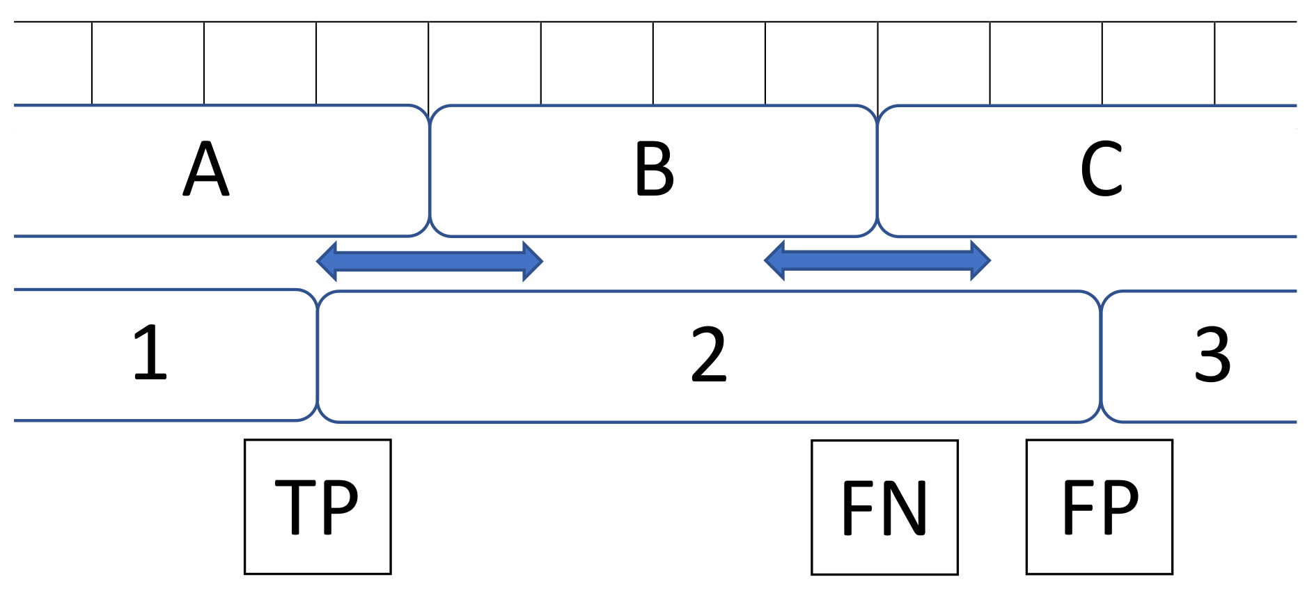
  77. Ward, J.A.; Lukowicz, P.; Gellersen, H.W. Performance Metrics for Activity Recognition. ACM Trans. Intell. Syst. Technol. 2011, 2, 6. [Google Scholar] [CrossRef]
Figure 1. An example of the clustering result for one DNA extraction experiment. Shown are the acceleration time series (orange, blue, green), ground truth labels (background colors) and transitions found from clustering (red vertical bars). Additionally, some video stills at the top show the process at different moments in time (arrows; l.t.r. : stirring, peeling, pestling, pouring). The cut marks are extracted from wrist acceleration measurements.
Informatics 05 00016 g001
Figure 2. The Grtool pipeline. Each step represents an independent, parallelizable module. Compare the supervised (top) and unsupervised (bottom) pipelines, where the train and predict steps in the former are replaced by the clustering step in unsupervised Activity Recognition (AR).
Informatics 05 00016 g002
Figure 3. The third dataset in this paper uses video frames from a Google Glass recording of steps in a thermoforming process, combined with IMU data from the wrist and Google Glass. Shown here are six distinct stills from the Google Glass video showing different actions (top) and wrist accelerometer data from the same recording (bottom time-series plot), with the process steps marked as background colors.
Informatics 05 00016 g003
Figure 4. Our approach matches individual activity labels (top: A, B and C) with clustered segments (bottom: 1, 2 and 3) to score transitions as true positives, false positives or negatives.
Informatics 05 00016 g004
Figure 5. Process benchmark of the CMU Kitchen experiments (y-axis log-scale). Durations (in s) of only the clustering process (top), as well as the whole experiment run (bottom), including preprocessing and feature extraction, are shown. Benchmarked algorithms are k-means (blue), agglomerative clustering (red) and GMM (green).
Informatics 05 00016 g005
Table 1. Results for individual top experiment runs (by recall), per dataset for unsupervised methods (the feature extraction window is the number of samples (@50 Hz ); the extracted feature is the mean, variance or time (time = mean/var/range/median); the transition scoring margin is the number of samples) (datasets numbered as listed in Section 4).
MethodModalityWindowFeatureMarginAccuracyRecallPrecision F 1 -Score
Set 1k-meanswrist acc80mean40.920.920.920.92
Agglo.wrist acc90time50.920.930.920.93
GMMwrist acc90mean30.880.880.870.87
Set 2k-meansl_leg mag100time30.970.970.980.97
Agglo.l_leg gyr100time30.970.970.980.97
GMMr_arm acc100var10.910.90.90.9
Set 3k-meanswrist acc80mean20.950.960.950.95
Agglo.head acc90mean20.950.960.950.95
GMMwrist mag100mean20.950.950.950.95
Table 2. Results for individual top experiment runs (by recall), per dataset for supervised methods, via the presented binary transition scoring (the feature extraction window is the number of samples (@50 Hz ); the extracted feature is mean, variance or time (time = mean/var/range/median); the transition scoring margin is the number of samples) (datasets numbered as listed in Section 4).
MethodModalityWindowFeatureMarginAccuracyRecallPrecision F 1 -Score
Set 1SVMwrist acc100time10.640.750.630.58
RFwrist acc100variance10.630.780.620.56
LDAwrist acc100variance10.680.780.670.64
QDAwrist acc90variance10.670.780.660.62
Set 2SVMl_arm acc90time10.710.70.690.68
RFr_arm acc100time10.820.830.820.82
LDAall100variance10.750.770.730.73
QDAr_arm mag50time10.670.790.660.63
Set 3SVMhead acc100time30.880.870.880.87
RFwrist acc100mean30.850.860.870.85
LDAwrist mag100mean20.850.870.860.84
QDAwrist mag60mean50.930.930.940.93
Table 3. Results for individual top experiment runs (by recall), per dataset for supervised methods, via classic multiclass scoring (the feature extraction window is the number of samples (@50 Hz ); the extracted feature is mean, variance or time (time = mean/var/range/median); the transition scoring margin is the number of samples) (datasets numbered as listed in Section 4).
MethodModalityWindowFeatureMarginAccuracyRecallPrecision F 1 -Score
Set 1SVMwrist acc20time-0.870.220.210.18
RFwrist acc100time-0.880.290.330.26
LDAwrist acc100time-0.880.320.330.3
QDAwrist acc100time-0.840.220.150.15
Set 2SVMr_arm acc100variance-0.910.060.020.03
RFr_arm acc100variance-0.940.020.020.02
LDAr_leg acc90time-0.920.10.050.06
QDAl_leg acc40mean-0.930.090.030.05
Set 3SVMhead acc70time-0.870.450.440.41
RFhead acc100time-0.860.450.530.44
LDAhead acc90time-0.880.490.530.48
QDAhead acc100mean-0.880.530.470.47
Table 4. Top scoring parameter combinations over all datasets (1/2/3) per method. The results show that these combinations have high scores for all datasets, not just individual experiments (the feature extraction window is the number of samples (@50 Hz ); the extracted feature is mean, variance or time (time = mean/var/range/median); the transition scoring margin is the number of samples) (datasets numbered as listed in Section 4).
MethodWindowFeatureMarginAccuracyRecallPrecision F 1 -Score
123123123123
k-means80mean40.920.880.950.920.880.950.920.890.950.920.880.95
Agglo.90time50.930.890.950.930.880.950.940.910.950.930.880.95
GMM90mean30.880.860.950.880.860.950.870.890.950.870.860.95
SVM (trans)80mean40.840.750.930.830.750.930.850.840.940.830.740.93
RF (trans)100variance10.680.910.710.800.920.820.680.910.710.640.910.69
Table 5. Results for individual top experiment runs (by recall), for selected methods on the DNA extraction dataset, while not excluding NULL samples (the feature extraction window is the number of samples (@50 Hz ); the extracted feature is mean, variance or time (time = mean/var/range/median); the transition scoring margin is the number of samples).
MethodModalityWindowFeatureMarginAccuracyRecallPrecision F 1 -Score
k-meanswrist acc90mean50.810.830.790.8
Agglo.wrist acc90mean30.830.830.810.82
GMMwrist acc90mean50.820.830.80.81
SVM (multi)wrist acc90time-0.960.170.20.18
RF (multi)wrist acc80variance-0.950.170.250.19

