
Enhanced Beetle Antennae Algorithm for Chemical Dynamic Optimization Problems’ Non-Fixed Points Discrete Solution


1
Institute of Artificial Intelligence, Guangxi University for Nationalities, Nanning 530006, China
2
Guangxi Key Laboratory of Hybrid Computation and IC Design Analysis, Guangxi University for Nationalities, Nanning 530006, China
3
School of Chemistry and Chemical Engineering, Guangxi University for Nationalities, Nanning 530006, China
4
School of Electronic Information, Guangxi University for Nationalities, Nanning 530006, China
*
Author to whom correspondence should be addressed.
Processes 2022, 10(1), 148; https://doi.org/10.3390/pr10010148
Submission received: 5 December 2021
/
Revised: 29 December 2021
/
Accepted: 5 January 2022
/
Published: 11 January 2022
(This article belongs to the Topic Bioreactors: Control, Optimization and Applications)
Abstract
:Dynamic optimization is an important research topic in chemical process control. A dynamic optimization method with good performance can reduce energy consumption and prompt production efficiency. However, the method of solving the problem is complicated in the establishment of the model, and the process of solving the optimal value has a certain degree of difficulty. Based on this, we proposed a non-fixed points discrete method of an enhanced beetle antennae optimization algorithm (EBSO) to solve this kind of problem. Firstly, we converted individual beetles into groups of beetles to search for the best and increase the diversity of the population. Secondly, we introduced a balanced direction strategy, which explored extreme values in new directions before the beetles updated their positions. Finally, a spiral flight mechanism was introduced to change the situation of the beetles flying straight toward the tentacles to prevent the traditional algorithm from easily falling into a certain local range and not being able to jump out. We applied the enhanced algorithm to four classic chemical problems. Meanwhile, we changed the equal time division method or unequal time division method commonly used to solve chemical dynamic optimization problems, and proposed a new interval distribution method—the non-fixed points discrete method, which can more accurately represent the optimal control trajectory. The comparison and analysis of the simulation test results with other algorithms for solving chemical dynamic optimization problems show that the EBSO algorithm has good performance to a certain extent, which further proves the effectiveness of the EBSO algorithm and has a better optimization ability.
1. Introduction
Chemical process control is a dynamic process in which state variables change over time and space dimensions are adjusted. As the problems of resource environments and biochemistry become increasingly prominent, the requirements for the optimization of the operating performance of the chemical process and the determination of control indicators are also increasing. The chemical control strategy of the traditional steady-state model to solve such problems cannot adapt to the overall dynamic behavior analysis and real-time control optimization of the system with the improvement of technology and cannot effectively solve the chemical process control problem. Therefore, dynamic optimization is an inevitable trend in the development of process control in the chemical industry.
Chemical engineering problems can be described as a class of complex nonlinear differential equations. The commonly used methods for solving dynamic optimization problems mainly include direct methods [1] and indirect methods [2]. The direct method transforms high-dimensional dynamic optimization problems into finite–dimensional static nonlinear programming problems through discretization, including the control variable parameterization method [3] (CVP), the iterative dynamic programming method [4] (IDP), complete parameterization [5], and so forth. The direct method has a strong dependence on the initial value, and for some non-continuous problems that cannot be derived, the solution value is inaccurate, the solution efficiency is low, and it cannot guarantee that the global optimal solution is located near the obtained control sequence. Moreover, the process of solving the state variable trajectory is more cumbersome. The indirect method takes the principle of extreme value as a necessary condition for the optimal control solution and converts the original problem into a two-point boundary value problem for the solution, including a finite element configuration [6] and the constant value insertion method, the univariate projection method [7], the multivariate projection method, and so forth. In engineering, to solve complex control systems, the indirect method has considerable limitations, and it is difficult to obtain a solution value. The direct method has become the mainstream method for solving dynamic optimization problems.
In recent years, intelligent optimization algorithms have sprung up rapidly. Compared to traditional solution methods, intelligent optimization has the following advantages: (1) the principle is simple and easy to implement; (2) the algorithm has better robustness and global convergence; (3) it does not require gradient information. Therefore, the numerical method of an intelligent optimization algorithm is widely used in dynamic optimization problems in various fields, and has gradually been extended to the solution of chemical dynamic optimization problems. Shi et al. [8] proposed a method based on PSO–CVP, using a particle swarm algorithm to solve the chemical process control, and feed the solution result to the control variable parameterization method for secondary optimization. Xu et al. [9] proposed a biogeographic learning particle swarm algorithm, which was combined with biogeographic learning methods to sort particles and improve learning efficiency. Tabassum et al. [10] proposed an improved differential gradient evolution method; the algorithm was combined with an improved dynamic probability distribution, enhanced exploration and development capabilities, and improved the premature convergence of the algorithm. It has good performance in complex nonlinear chemical design problems. Pham et al. [11] proposed smoothing and rotation into genetic algorithms to increase the diversity of the population and to solve the problem of chemical dynamic optimization. Zhang et al. [12] introduced a sequence ant colony optimization algorithm to solve the chemical dynamic problem. In the solutions of dynamic optimization problems, the intelligent optimization algorithm can converge to the global optimum according to the probability. Appropriate improvement of the algorithm can prevent it from falling into the local optima. At the same time, the bionic random mechanism of the intelligent algorithm faces the problem of slow convergence speed and low optimization efficiency. The bottleneck restricts its real-time application in engineering.
For this reason, we started from the perspective of improving the algorithm’s slow convergence speed and low solution accuracy in chemical dynamic optimization problems. We proposed an enhanced beetle algorithm based on the discretization of a non-fixed points segmentation method. In this way, problems such as a lack of population diversity and falling into the local optima prematurely can be solved. Firstly, we converted individual beetles into beetle swarms to search for the best solution and to increase the diversity of the beetle populations. Secondly, we introduced a balanced direction strategy so that the beetles can explore extreme values in new directions before updating their positions. Finally, the spiral flight mechanism was introduced to change the situation of the beetle flying in the direction of the antennae in a straight line to prevent the traditional algorithm from easily falling into a certain local area and not being able to jump out. The enhanced algorithm was subjected to benchmark test function experiments and combined with the random point method to solve four typical chemical dynamic optimization examples. By comparison and analysis of different algorithms, the results show that the EBSO algorithm has better optimization performance, and satisfactory experimental results were obtained, supporting key application advantages in solving chemical dynamic optimization problems.
The paper is organized as follows: Section 2 describes the dynamic optimization problem and the non-fixed points discrete method, which are compared with the equal division method and the unequal division method. Section 3 briefly reviews the classic beetle antennae search algorithm and its process. Section 4 explains the main contribution of this paper, which is the enhanced beetle algorithm, and describes the benchmark function tests performed on it. Section 5 uses the EBSO algorithm to calculate the experimental results on the four chemical dynamic optimization cases.
2. Problem Description and Non-Fixed Points Discrete Method
2.1. Description of Dynamic Optimization Problem
The dynamic optimization problem (DOP) means that the optimal control range gradually tends to the current dynamic operating volume under the condition of safety and constraints [13]. The research object is usually a time-varying system in mathematics. The mathematical model of the dynamic optimization problem is described as a differential–algebraic optimization problem, which dynamically solves the optimal solution of general dynamic optimization problems [14]. The mathematical model of the dynamic problem describes the goals as follows:
where is the performance index, is the differential equation constraint, represents the state variable, and is the starting value of the state variable at time , represents the control variable, and respectively represent the upper and lower bounds of the control variable, and respectively represent the minimum and maximum value of the state variable, and and respectively represent the start and end time of the reaction process. Solving the dynamic optimization problem requires finding the optimal control strategy to minimize the performance index obtained by the process under the condition of satisfying the constraints.
2.2. Non-Fixed Points Discrete Division Method
According to the analysis of the above dynamic optimization model, the dynamic optimization problem can be transformed by the parameterization of the control vector. The parameterization of the control vector involves the use of a limited number of parameters to approximate the control vector , which changes continuously with time. The time interval is usually divided into sub-intervals to solve the problem of the control trajectory change problem. Currently, the equal division method [8,15] and the unequal division method [16] are mostly used for the division of time intervals in dynamic optimization. Israel et al. [17] used the derivative-free trust region algorithm to divide the time interval to solve the dynamic optimization problem. Tian et al. [18] used the symbiosis algorithm to solve the problem of equal division of the time interval for an appropriate solution. The time interval is equally divided, the length of each sub-region is , and each sub-region is solved by the Runge–Kutta method. At the same time, the corresponding method is used to optimize the control variables so that the control variables produce a series of trajectories. However, compared to the equal time interval distribution, the variable time interval distribution can produce a more precise control trajectory by adjusting the length of the sub-intervals, thereby obtaining a better solution effect. Xu et al. [19] used an improved seagull optimization algorithm to solve the chemical dynamic optimization problem with the unequal division of the time interval and obtained better test results. The unequal division of the time interval involves initializing a set of parameters in the time domain according to certain rules, namely , the division formula of the unequal division method [19], as follows:
Unequal division is based on equal division, and the length of each segment is changed into an increasing interval length according to an equal interval. The Runge–Kutta method is used [20] to solve each sub-interval obtained after division and to obtain the running trajectory generated by the control variable.
Based on the idea of the piecewise constant method in the parameterization of control variables, we proposed a new method of determining time nodes in the time domain—the non-fixed points discrete method. The basis of the idea is to randomly broadcast time separation points within the start and end time interval of the reaction process. The distance between two different adjacent points may be longer or shorter, and the position of the nodes may be sparse or dense. The is calculated in turn to obtain the control trajectory. Compared to the equal division method and the unequal division method, the non-fixed points discrete method determines the time node more randomly. Equal length interval division and unequal length interval division are used to solve the location of specific time nodes. The non-fixed points discrete method can refine the control process due to the randomness of the scattered points, produce a more precise control trajectory, and more closely match the actual control variable changes, eventually obtaining better performance indicators. Figure 1 is a comparison diagram of three different types of division. Figure 2, Figure 3 and Figure 4 are the model diagrams of the division methods of different point setting methods.
It can be seen from the figures above (Figure 1, Figure 2, Figure 3 and Figure 4) that the selection of the dividing points for the equal division is a fixed value within the range. According to Formula (3), the distance between the adjacent division points of the unequal division is shown to increase according to the discipline, and the position of the division point can be calculated. The method proposed in this paper can be used to determine the time sub-interval based on random points by randomly selecting the value of the division point within the interval. As shown in Figure 4, the division points can be sparse in one part and dense in the other part. Such a division method has better randomness compared to equal and unequal division, which can calculate the fitness value of the positions of the fixed points and, meanwhile, avoid only calculating the value of the related control variable at the fixed position, more accurately reflecting the reaction situation in the chemical process control. At the same time, the Runge–Kutta method is used to solve each sub-interval . Finally, according to the function approximation theory combined with the EBSO algorithm proposed in this paper, each optimal result is approximated by a linear combination to obtain the optimal control variable result.
3. Beetle Antennae Optimization Search
Beetle antennae search (BAS) [21] is a heuristic optimization algorithm proposed by Jiang and Li. The algorithm uses a mathematical model established by simulating the foraging behavior of beetles to optimize and solve complex problems. In the process of foraging, beetles do not know the location of the target food source, but use the two antennae on their heads to gather the strength of the smell to forage. When the intensity of the smell received by the beard on the left is greater than that on the right, the beetles will fly to the left in the next step; otherwise, they will fly to the right. According to this principle, beetles can effectively find food. The bionic behavior diagram is shown in Figure 5.
3.1. Basic Principles
The foundation of this algorithm is that the smell of food is equivalent to a function. Each point value of the function is different in space. The beetles’ two antennae can collect the smell values of two points nearby. The purpose of the beetles is to find the point with the highest smell value in the search range. The specific orientation of food is equivalent to the maximum point of the objective function, and the smell is equivalent to the function itself. Beetles move step by step to the orientation with the heaviest food smell. The beetle antennae optimization algorithm is different from other optimization algorithms. The beetle antennae search only needs one individual, that is, one beetle, and the amount of computation is greatly reduced.
Therefore, the process of beetle foraging is the optimization process of the beetle antennae algorithm. The steps are as follows:
The following is the initial position vector of the beetle:
where is the random function and is the dimension of space. For the selection of step factor , the initial step can be as large as possible, preferably equivalent to the maximum length of the independent variable. Equation (5) is used in each iteration, as follows:
The value range of decline factor is between , usually taken as . is the current number of iterations and is the total number of iterations.
The following are the position coordinates of the left and right antennae of beetle:
where represents the coordinate position of the left antennae, represents the coordinate position of the right antennae, represents the centroid coordinate of the beetle in the times iteration, and represents the distance length between the left and right antennae. We set its value large enough to cover part of the search interval—.
The fitness function , where represents the odor concentration values to be obtained, is expressed as and respectively. The fitness function is determined according to the actual needs, and its selection is described later.
The beetle position is updated by comparing the fitness values of the left and right antennae. If , the beetle moves to the left; if it is the opposite, the beetle moves to the right. The following is the next position update formula:
where represents the step size factor of times the iterations. In this paper, we set the initial beetle step size as , and is the symbolic function to return the positive and negative of the parameter value.
3.2. Performance Analysis
The algorithm relies on the left and right antennae of the beetle to distinguish the odor intensity of the food obtained from their respective positions. Although the algorithm can quickly speed up the update and optimization of the beetle position, it will cause the beetle to fall into the local minima, and the beetle will not jump out of the local area. For optimal ability, the beetle moves in a single random direction in each iteration, but there is no guarantee that the movement of the beetle will make the objective function value better. Therefore, the results of the BAS algorithm are different each time. Secondly, the BAS algorithm is a search algorithm for an individual beetle. A single beetle has a weak ability to distinguish food odor concentration in a high-dimensional space, making it difficult to find the optimal solution in such a space, completely falling into the local minima, and weakening the search ability of the algorithm in the space. The pseudo-code of the BAS algorithm is shown in Algorithm 1:
| Algorithm 1: BAS Algorithm |
| Initialize the position of beetle ; Assign free parameters—the distance between the beetle’s two antennae ; step size ; max iteration ; spatial dimension ; 1. Calculate the fitness of the : ; 2. for = 1 to ,  9. End for 10. Update the step size by Equation (5); 11. = the fitness of the best value; 12. Return . |
4. Enhanced Beetle Antennae Optimization Algorithm (EBSO)
In the search space of different dimensions, the typical beetle antennae algorithm a has fast convergent solution and less time-consuming search capabilities. However, due to the complex dynamic optimization control system, the BAS algorithm will lose its own advantages in some cases, making it computationally inefficient and time-consuming, especially for complex engineering optimization problems. The main reason is that in the beetle antennae algorithm, the beetle directly flies in the direction of its antennae based on its individual optimization and position update, eventually resulting in a decrease in the solution value diversity of a later iteration. With an in-depth analysis of the beetle antennae algorithm and dynamic optimization problems, we proposed the following improvement strategies for the beetle antennae algorithm, which greatly improve the solution performance of the BAS algorithm.
4.1. Beetle Swarm
The typical beetle antennae algorithm involves finding the best solution result based on a single beetle search. It can quickly obtain approximate solutions for simple function-solving problems. However, as the problem scale and the variable dimensions increase, the solution accuracy of the BAS algorithm gradually decreases, and the convergence effect becomes worse. Meanwhile, the individual beetle searches for optimization in a single direction in each iteration, while there is no guarantee that the individual beetle will have a better objective function value for each optimization. Aiming at the shortcomings of the beetle antennae algorithm, we optimized a single beetle into a group search model. beetles move in directions to speed up the beetle group’s search for the global optimum, thereby improving the possibility of a beetle finding a better position and avoiding falling into the local minima.
The beetle swarm can be expressed as follows:
where represents the population number of beetles and represents the dimension of the optimization problem. The direction vector of each beetle is expressed as follows:
The fitness value corresponding to the beetle population can be represented by the following vector:
The value of each column in represents the fitness value of the corresponding individual beetle. By transforming a single beetle into a group beetle search, the algorithm’s optimization ability in the search process is greatly improved, the search range is expanded, and a better solution is produced.
4.2. Balanced Direction Strategy
Before updating the position, the beetle processes its left and right antennae to explore the food smell, that is, the fitness value of the left and right antennae, and then decides the direction of the next flight. Due to the position of the two antennae, a single position is determined according to the direction. In order to allow the beetle to explore more positions, a balanced direction strategy was introduced to make the next flight direction of the beetle more random. The following adjustments were made to Formulas (4) and (5):
where is a random factor, represents the step length of the beetle, and the step size update is used to adjust it accordingly with Formula (5); is described in detail below. is a balance factor combined with the step size and is used to adjust the direction of the beetle. represents the current global optimal solution, and represents the current local maximum value. The local and global extreme values are adjusted through the balance direction strategy to make the next flight direction of the beetle more random.
According to the simulation principle of a typical beetle antennae algorithm, two important parameters affecting the performance of the algorithm are the step size of the beetle position update and the moving flight direction. In order to make the algorithm have a better optimization effect in solving the chemical dynamic optimization problem, these two parameters were modified to some extent. According to Formula (5), the step size of a beetle decreases monotonically and linearly. The larger the step size is, the stronger the global search ability is. In contrast, the smaller the step size is, the stronger the local search ability of beetle is. Therefore, the BAS algorithm has the disadvantage of a slower convergence speed in the later stage, which makes it easily fall into the local minima and have low solution accuracy. In order to ensure the calculation efficiency and overcome the above problems, the step size of the beetle position update can be dynamically adjusted. Formula (5) was changed as the step size of Formula (11) to improve the performance of the algorithm. In the early stage of the algorithm optimization, the beetle can expand the search range in the solution space to quickly find the optimization. The beetle uses a large step size factor in the later stage of the algorithm optimization. Once the search solution is stabilized, and in order to make the optimization more accurate, the beetle uses a small step size factor. The original step size and the decreased dynamic balance adjustment step size are shown in Figure 6.
It can be seen from Figure 6 that the step size of the typical beetle antennae algorithm decreases monotonously and changes uniformly each time. A beetle can easily explore a certain range and fall into local minima, leading to an error in the solution. With the introduction of the dynamic balance adjustment mechanism, the step size of the beetle antennae algorithm can perform a large-scale spatial search at the beginning of the search. When the iteration reaches the middle times, the step size becomes shorter and faster, causing the search range to shrink. In the later stage of the iteration, the step size is shortened and weakened, which makes the algorithm search and optimization more accurate, enriches the global search ability, and improves the search accuracy.
4.3. Introducing the Spiral Flight Mechanism
According to the typical beetle antennae algorithm, the beetle decides the next direction according to the fitness values of the left and right positions, and moves according to the step size, which leads to the single-direction update of the beetle’s position and makes it easy to fall into the local extreme value. For this reason, the spiral motion of hunting behavior [22] in the whale optimization algorithm is introduced in the step of updating the position of the beetle. When the beetle is flying to the next step, it will fly to the food in a spiral motion. The spiral motion behavior in the plane is described as follows:
where is the radius of each spiral, and is the random angle value within the range . is a constant, usually assigned to ; it is used to define the shape of the spiral. and are the relevant constants of the spiral shape, and is the base of the natural logarithm. Therefore, the updated mathematical model of the beetle position Formula (8) with the introduction of the spiral flight mechanism is as follows:
By introducing the performance enhancement of the typical beetle antennae optimization algorithm, the EBSO algorithm we proposed was obtained. The EBSO algorithm can effectively solve complex engineering dynamic optimization problems. The pseudo-code of the enhanced beetle algorithm is shown in Algorithm 2:
| Algorithm 2: Enhanced Beetle Antennae Optimization Algorithm (EBSO) |
| Input: Establish an objective function ; Output: Optimal search agent and fitness value of optimal position zbestValue; 1. Procedure EBSO 1. Initialize parameters, mainly including , , , , , and initialize beetle positions , where is the number of the population; 2. Randomly generate division points in the time interval; 3. Apply CalculateFitness function to calculate fitness value; 4. Use FindZbest function to find zbest and zbestValue;  15. End for 16. Output global optimal value; 17. End Procedure. 2: Procedure CalculateFitness 1. Initialize spatial dimension , which represents the dimension of problem;  7. return ; 8. End Procedure. 3: Procedure FindZbest 1. zbestValue = ;  8. Return , zbestValue; 9. End Procedure. |
4.4. Benchmark Functions
In order to test the feasibility and effectiveness of the EBSO algorithm, we tested the improved algorithm with 10 well-known benchmark functions, as shown in Table 1. The simulation software used in the experiment was MATLAB R2018a.
4.4.1. Parameter Settings
To verify the excellent performance of the EBSO algorithm, we selected several typical meta-heuristic algorithms for comparison, including particle swarm optimization (PSO) [23], the traditional beetle antennae algorithm (BAS), the whale optimization algorithm (WOA), and the ant lion optimizer (ALO) [24]. In order to make the algorithm obtain satisfactory results and ensure fairness, the maximum number of iterations of each algorithm was 200. The search population of each algorithm was 100. The specific parameters of the relevant algorithm included the following: for the PSO, the learning factors and were 2, and the inertia factor was 0.8; for the BAS, the initial step size was set to 1, each function was run 20 times, and the average, optimal, and worst values of the five algorithms were respectively counted.
4.4.2. Statistical Result Comparison
Each algorithm was run independently 20 times, and the average value, optimal value, and worst value of the five algorithms were counted respectively. The results of the test are listed in Table 2. From the experimental results, we can see the optimization performance of the EBSO algorithm.
According to the data in Table 2, the benchmark test functions , , , , and were run independently 20 times, and the EBSO algorithm could solve the optimal value each time. Some of the results of the benchmark test functions and could be solved to the optimal solution; meanwhile, the average solution value was nearly 10 times higher than the other four algorithms in solution accuracy. Although the solution results of the benchmark test functions , , and do not reach the optimal solution, the accuracy of the solution was greatly improved compared to the traditional beetle antennae algorithm, and it was better than the solution result of the whale optimization algorithm, with an increase of about 6–170 orders of magnitude. In order to show the excellent performance of the EBSO algorithm more intuitively, Figure 7, Figure 8, Figure 9, Figure 10, Figure 11, Figure 12, Figure 13, Figure 14, Figure 15 and Figure 16 show the iterative convergence diagrams of the five algorithms. To show the convergence effect of the algorithms more clearly, some functions adopted logarithmic function expressions for fitness values.
According to the iterative convergence graph of 10 benchmark test functions for five optimization algorithms, it can be seen that the test functions , , , and could be solved to the optimal solution after about 160 iterations. Functions , , , , and had better solution accuracy and faster convergence speed due to the rapid convergence of the beetle antennae algorithm. For function , the EBSO algorithm had a slightly worse convergence effect than the PSO algorithm at the beginning of the iteration. This is because the EBSO algorithm needs to be determined at the beginning of the iteration. Once the target orientation is determined, the variable energy can quickly converge and be solved. At the same time, for the test function , the EBSO algorithm can solve the optimal solution -1, and the solution results of other algorithms cannot reach the optimal solution. Through the above analysis, the effectiveness of the EBSO algorithm in this paper is further proved. It also provides a feasible basis for the enhanced beetle antennae algorithm to solve the complex control equations in the chemical process control.
5. Application of EBSO Algorithm in Chemical Process Control
The EBSO algorithm achieved relatively ideal performance results in the benchmark test. Next, we tested whether the EBSO algorithm still has good solution performance in chemical dynamic optimization problems. In this study, we chose common cases in chemical problems for optimization, including inequality constrained optimization, a batch reactor, a tubular reactor, the parallel reaction of a tubular reactor, and so forth. When using the EBSO algorithm to solve chemical problems, the control time interval is divided into segments according to random points, and each point is randomly selected within the interval, . Then, the control variable is expressed as a constant function in each interval, namely , which represents the solution of the optimized objective function. Finally, each interval is solved by the EBSO algorithm.
5.1. Experimental Process Analysis
The specific process steps of using the proposed EBSO algorithm to solve the chemical process control optimization problem are as follows:
- The optimization problem of chemical process control is segmented by the random point method. The number of segments is N.
- We used the Runge–Kutta method to solve each segment after segmentation.
- We used the EBSO algorithm to optimize different chemical reactors.
In the EBSO algorithm, the position information of the beetle swarm was expressed as the optimal control variable. The product concentration of the chemical reactor was used as the fitness function value of the optimization algorithm. Each chemical reactor was operated independently 20 times. The data presented below are the average values of 20 iterations. The specific flow chart of the experiment is shown in Figure 17. The specific experiment parameters were set as shown in Table 3.
5.2. Test Case and Analysis
5.2.1. Case 1: Inequality Constrained Optimization
This example is a classical dynamic optimization problem in chemical process control. It consists of a mathematical system without equality constraints. The optimization problem contains two state variables and solves the minimum value of one state variable under the condition. The mathematical model of the problem is as follows:
where and are the two state variables of the problem model, is the control variable, and represents the termination time of the process. Using the enhanced beetle antennae optimization algorithm based on the non-fixed points discrete method, the calculation results of different segments of the model are shown in Figure 18, Figure 19 and Figure 20.
The comparison of solution results of different algorithms for the chemical control problem is shown in Table 4.
According to the above experimental data, with the increasing number of segments in the time interval, the calculation results are more accurate, but the more segments, the more time-consuming the calculation was. In random scatter segments , , , and , the EBSO algorithm obtained better results when . This is not available in other algorithms. When , the optimal junction value reached 0.76135774, which is more accurate than other algorithms in segments. This gives full play to the advantages of the fast convergence optimization and improved strategy of the beetle antennae algorithm.
5.2.2. Case 2: Batch Reactor Consecutive Reaction ()
A batch reactor is common equipment in chemical production. The temperature control of a batch reactor is the key to producing qualified products and improving product quality. After the reaction material is put into the equipment, in order to reach the reaction temperature, it needs to be provided with a certain amount of heat before the reaction starts. Once the reaction temperature is reached, it will release heat continuously with the progress of a chemical reaction. In this process, the reactor temperature needs to be controlled to avoid potential safety hazards. In the reaction process of a batch reactor, is used as the raw material to produce target product and by-product , so as to maximize the concentration of target product at the end of the reaction. That is, the reaction temperature needs to be controlled in this process to make the concentration of reach the optimal value at the end of the reaction. The device of the reactor is shown in Figure 21. The mathematical model [25] of the reactor problem is shown as follows:
where and represent the concentrations of reactant and target product , respectively, is the reactor temperature control, and represents the reaction terminal time. The greater the time division number is, the higher the accuracy of the control strategy is and the greater the calculation is. Its value should be selected according to the actual needs. In order to better form the comparison of experimental results, we selected , and other segments to summarize. The EBSO algorithm was tested and analyzed with Case 1, and the results were compared with other algorithms to solve Case 1. These include the following: Zhang et al. [12] proposed a sequential execution ant colony (SACA); Peng et al. [15] proposed an improved knowledge evolution algorithm (IKEA); Sun et al. [30] proposed a differential evolution algorithm based on control variable parameterization (CVP-DE); Liu et al. [31] proposed an improved knowledge guided culture algorithm (IKBCA); Mo et al. [32] proposed an adaptive cuckoo algorithm (VSACS); Renfro et al. [33] proposed a method combining quasi-Newton and global spline sampling; Zhang et al. [34] proposed an iterative ant colony algorithm (IACA); Jiang et al. [35] proposed an artificial raindrop algorithm (MOARA) and other relevant paper data.
When the number of segment points is , the reactant concentration results produced by different algorithms are shown in Table 5. The optimal temperature control sequence, iterative convergence diagram, and optimal trajectory of state variables in the process of EBSO reaching the optimal concentration are shown in Figure 22 and Figure 23.
When the number of segment points is , the reactant concentration results produced by different algorithms are shown in Table 6. The optimal temperature control sequence, iterative convergence diagram, and optimal trajectory of state variables in the process of EBSO reaching the optimal concentration are shown in Figure 24 and Figure 25.
The comparison of other segment points and the algorithm comparison results of different segment numbers are shown in Table 7. The optimal concentration is shown in Figure 26. We present Figure 27 to more clearly observe the difference between the solution results of the EBSO algorithm and the other algorithms.
It can be clearly seen from Figure 27 (green bar column) that the accuracy of our proposed EBSO algorithm in solving for a batch reactor is higher than that of other algorithms.
By comparing the experimental results of the test batch reactor under different numbers of segments, it can be concluded that the EBSO algorithm proposed by us has a better optimal solution when the segment numbers are , , and other segments. In the case of , compared to the other six methods for solving for a batch reactor, the solution results of EBSO show relatively excellent performance, and the best value is 0.610558922, while the results of other algorithms are mostly 0.6101, and the solution accuracy of the EBSO algorithm has been significantly improved. In the case of , compared to the other six algorithms, the optimal solution of the EBSO algorithm is 0.61064758, but the optimal value of the other algorithms is about 0.6104. Further comparing the solution results of other numbers of segments, different algorithms refined the temperature control with the increase in the number of segments, and the solution accuracy was improved accordingly. Similarly, the results of obtaining the optimal value of EBSO were further improved. Taken together, these results suggest that EBSO has good performance for solving for batch reactors.
5.2.3. Case 3: Tubular Reactor ()
A tubular reactor is also called a catalyst mixing problem. This optimization problem was proposed by Gunn [38] et al.; there is a mixture of two catalysts that react under its action (). The optimal control problem involves the maximization of the production of product under a given reactor length, and can be further improved by changing the catalyst mixture along the reactor. The mole fractions of substances and in the mixture are represented by and , respectively, and it is assumed that all reactions are carried out in an isothermal tubular reactor. Then, the mathematical model of the optimization problem of maximizing the concentration of the final product is as follows:
where is the length of the tubular reactor, and represents the content of the first catalyst in the tube from the starting point . In order to improve the utilization of raw materials and obtain the maximum concentration of target product at the end of the reaction, it is necessary to optimize the distribution of catalyst in the tube. The model diagram of tubular reactor is shown in Figure 28.
The EBSO algorithm was used in the experiment of process control reaction of the tubular reactor. The number of beetle populations was 100 and the maximum number of iterations was 100. The example was tested 20 times independently and the average result was selected. In order to better form the comparison of experimental results, , , and other segments were summarized in this paper.
The reactant concentration results produced by different algorithms are shown in Table 8 for when the number of segment points was . The optimal temperature control sequence and the iterative convergence diagram of EBSO reaching the optimal concentration are shown in Figure 29.
The reactant concentration results produced by different algorithms are shown in Table 9 for when the number of segment points was . The optimal temperature control sequence, the iterative convergence diagram, and the optimal trajectory of state variables in the process of EBSO reaching the optimal concentration are shown in Figure 30 and Figure 31.
The comparison of other segment points and the algorithm comparison results of different segment numbers are shown in Table 10.
The optimal control sequence and iterative convergence diagram are shown in Figure 32 for when the random points were .
We present Figure 33 to more clearly observe the difference between the solution results of the EBSO algorithm and the other algorithms.
It can be seen from Figure 33 (green bar column) that the EBSO algorithm we proposed has good computational performance in solving for the tubular reactor. Only when the number of discretization points is , the solution value is slightly worse than that of the PWV–CVP algorithm.
By comparing the results obtained in different random segments of the test tubular reactor, it can be seen that the EBSO algorithm has good optimization results. When the random point value was , the calculation result of EBSO reached 0.47502183, while the results of the compared algorithm were around 0.7363, which is more accurate than that of the IKEA algorithm. When the random point was , the optimization results of the compared algorithms were improved. Only the solution value of the EBSO algorithm reached 0.47627191, and the other algorithms were around 0.47527. The comparison of the solution of other algorithms with different segment numbers is shown in Table 9. Taken together, these results suggest that the EBSO algorithm has good solution results in low segment numbers to a large number of random segments, which further proves the effectiveness of the EBSO algorithm proposed in this paper.
5.2.4. Case 4: Parallel Reaction Problem of Isothermal Tubular Reactor ()
In an isothermal tubular reactor, there is a parallel reaction process in which reactant can produce target products and or more different products at the same time. This parallel reaction process is described as (). After the end of the reaction process, the concentration of target product is maximized. This process is called the main reaction. The process of producing other products from reactant is called the side reaction.
The model of the process control optimization problem is as follows:
where represents the concentration of reactant and represents the concentration of substance produced by the main reaction in the product. represents the saturation of the control variable, is the control time at the end of the reaction, is the performance index, and the control process involves solving the control time to get the maximum concentration of , that is, .
Similarly, in the experiment of the parallel reaction process of an isothermal tubular reactor using the EBSO algorithm, the number of beetle populations was set as 100 and the maximum number of iterations was 100. The example was tested independently 20 times and the average result was selected. In order to better form the comparison of experimental results, , , , and other segments are summarized in this paper.
The optimal temperature control sequence and iterative convergence diagram of EBSO reaching the optimal concentration are shown in Figure 34 for when the number of segment points was .
The optimal temperature control sequence and iterative convergence diagram of EBSO reaching the optimal concentration are shown in Figure 35 for when the number of segment points was .
The optimal temperature control sequence, iterative convergence diagram, and optimal trajectory of state variables in the process of EBSO reaching the optimal concentration are shown in Figure 36 and Figure 37 for when the number of segment points was .
The comparison of the optimization results of different algorithms for the chemical process control problem is shown in Table 11. Figure 38 shows the solution statistics of the EBSO algorithm and other algorithms when .
By comparing the results of different random segments of an isothermal tubular reactor in parallel reaction, it can be seen that the EBSO algorithm proposed by us has good optimization results. When the random point value was , the EBSO calculation result reached 0.57317785, while the comparison algorithm results were near 0.5722. When the random point was , the optimization results of the compared algorithms were improved. Only the solution value of EBSO algorithm reached 0.57412271, and the other algorithms were near 0.573. Other different algorithms in Table 10 solved the process control results. From the data, it can be seen that the solution results are somewhat different from the EBSO algorithm. The EBSO algorithm has good results in a low to high number of random segments, which further proves the effectiveness of the EBSO algorithm proposed in this paper.
6. Conclusions
In this paper, an enhanced beetle antennae optimization algorithm is proposed to solve the dynamic optimization problem in chemical process control. By changing the typical equal division method and unequal division method commonly used in solving chemical dynamic optimization problems, a new interval division non-fixed points discrete method is proposed. The discretized segmentation points are randomly generated in the time region without any law. In this way, the control process is refined, a more precise control trajectory is generated, and a better performance index is obtained. The individual beetle is transformed into a beetle swarm for search optimization, and the balance direction strategy is introduced to change the direction of the beetle when updating its position so as to increase the population diversity. The spiral flight mechanism is introduced to make the beetle have the ability of spiral flight when updating the position so as to overcome the defect that makes it easy for it to fall into local minima in the original algorithm. The enhanced beetle antennae algorithm can be applied to solve typical chemical dynamic optimization problems. The experimental results show that the EBSO algorithm has good performance.
In the future, we will do more research (1) to further optimize the reactor dynamic optimization problem of chemical process control with constraints; (2) to study and discuss new methods of time interval division, such as random segmentation method, and the matching and coordination between determining the optimal number of segments and the number of random segments and the population number and spatial dimension of an intelligent optimization algorithm.
Author Contributions
Conceptualization, Y.L. (Yucheng Lyu) and Y.M.; methodology, Y.L. (Yucheng Lyu); software, R.L.; validation, Y.M. and Y.L. (Yanyue Lu); writing—original draft preparation, Y.L. (Yucheng Lyu); writing—review and editing, Y.L. (Yucheng Lyu) and Y.M.; supervision, Y.M. All authors have read and agreed to the published version of the manuscript.
Funding
This research was supported by the National Science Foundation of China under grant no. 21466008, funder: Yuanbin Mo, and grant no.21968008, funder: Yanyue Lu; by the Project of the Natural Science Foundation of Guangxi Province under grant 2019GXNSFAA185017, funder: Yuanbin Mo, and by the Scientific Research Project of Guangxi University for Nationalities under grant 2021MDKJ004, funder: Yuanbin Mo.
Institutional Review Board Statement
Not applicable.
Informed Consent Statement
Not applicable.
Data Availability Statement
Not applicable.
Acknowledgments
This research was supported by the National Natural Science Foundation of China, grant numbers 21466008, 21968008, the Guangxi Natural Science Foundation of China, grant number 2019GXNSFAA185017, and the Scientific Research Project of Guangxi University for Nationalities, grant number 2021MDKJ004.
Conflicts of Interest
The authors declare no conflict of interest.
References
- Peng, H.J.; Gao, Q.; Wu, Z.G.; Zhong, W.X. A Mixed Variable Variational Method for Optimal Control Problems with Applications in Aerospace Control. Zidonghua Xuebao/Acta Automatica Sinica 2011, 37, 1248–1255. [Google Scholar]
- Sun, Y.; Zhang, M.R.; Liang, X.L. Improved Gauss Pseudospectral Method for Solving Nonlinear Optimal Control Problem with Complex Constraints. Acta Automatica Sinica 2013, 39, 672–678. [Google Scholar] [CrossRef]
- Xu, W.F.; Jiang, A.P.; Wang, H.K.; Jiang, E.H.; Ding, Q.; Gao, H.H. A Grid Reconstruction strategy based on Pseudo Wigner-Ville Analysis for Dynamic Optimization Problem. CIESC J. 2019, 70, 158–167. [Google Scholar]
- Mekarapiruk, W.; Luus, R. Optimal Control by Iterative Dynamic Programming with Deterministic and Random Candidates for Control. Ind. Eng. Chem. Res. 2000, 39, 84–91. [Google Scholar] [CrossRef]
- Liu, X.G.; Chen, L.; Hu, Y.Q. Solution of Chemical Dynamic Optimization Using the Simultaneous strategies. Chin. J. Chem. Eng. 2013, 21, 55–63. [Google Scholar] [CrossRef]
- Virginie, M.; Jacques, J.; Girault, H.H. Mixing Processes in a Zigzag Microchannel: Finite Element Simulations and Optical Study. Anal. Chem. 2002, 74, 4279–4286. [Google Scholar]
- Daszykowski, M.; Kacamarek, K.; Vander Heyden, Y.; Walczak, B. Robust statistics in data analysis—A review: Basic concepts. Chemom. Intell. Lab. Syst. 2007, 85, 203–219. [Google Scholar] [CrossRef]
- Shi, B.; Yin, Y.; Liu, F. Optimal control strategies combined with PSO and control vector parameterization for batchwise chemical process. CIESC J. 2019, 70, 979–986. [Google Scholar]
- Xu, C.; Mei, C.; Xu, B.; Ding, Y.; Liu, G. Biogeography-based learning particle swarm optimization method for solving dynamic optimization problems in chemical processes. CIESC J. 2017, 68, 3161–3167. [Google Scholar]
- Tabassum, M.F.; Saeed, M.; Akgül, A.; Farman, M.; Akram, S. Solution of chemical dynamic optimization systems using novel differential gradient evolution algorithm. Phys. Scr. 2021, 96, 035212. [Google Scholar] [CrossRef]
- Pham, Q.T. Dynamic Optimization of Chemical Engineering Processes by an Evolutionary Method. Comput. Chem. Eng. 1998, 22, 1089–1097. [Google Scholar] [CrossRef]
- Zhang, B.; Yu, H.; Chen, D. Sequential Optimization of Chemical Dynamic Problems by Ant-Colony Algorithm. J. Chem. Eng. Chin. Univ. 2006, 20, 120–125. [Google Scholar]
- Vicente, M.; Sayer, C.; Leiza, J.R.; Arzamendi, G.; Lima, E.L.; Pinto, J.C.; Asua, J.M. Dynamic. Optimization of Non-Linear Emulsion Copolymerization Systems: Open-Loop Control of Composition and Molecular Weight Distribution. Chem. Eng. J. 2002, 85, 339–349. [Google Scholar] [CrossRef]
- Mitra, T. Introduction to dynamic optimization theory. In Optimization and Chaos; Springer: Berlin/Heidelberg, Germany, 2000; pp. 31–108. [Google Scholar]
- Peng, X.; Qi, R.B.; Du, W.L.; Qian, F. An Improved Knowledge Evolution Algorithm and its Application to Chemical Process Dynamic Optimization. CIESC 2012, 63, 841–850. [Google Scholar]
- Zang, R.L.; Li, S.R.; Ge, Y.L.; Chang, P. An Improved Krill Herd Algorithm for Solving Chemical Dynamic Optimization Problems. J. Syst. Sci. Math. Sci. 2016, 36, 961–972. [Google Scholar]
- Israel, N.O.; Antonio, F.T.; Miguel, A.G.-L. Dynamic Optimization of a Cryogenic Air Separation Unit Using a Derivative-free Optimization Approach. Comput. Chem. Eng. 2017, 109, 1–18. [Google Scholar]
- Peng, T.; Xu, C.; Zhao, W.X.; Du, W.L. Dynamic Optimization of Chemical Processes Using Symbiotic Organisms Search Algorithm. In Proceedings of the Chinese Automation Congress (CAC), Hangzhou, China, 22–24 November 2019. [Google Scholar]
- Xu, L.; Mo, Y.B.; Lu, Y.; Li, J. Improved seagull Optimization Algorithm Combined with an Unequal Division Method to Solve Dynamic Optimization Problems. Processes 2021, 9, 1037. [Google Scholar] [CrossRef]
- Kedir, A.K. Numerical Solution of First Order Ordinary Differential Equation by using Runge-Kutta Method. Int. J. Syst. Sci. Appl. Math. 2021, 6, 1–8. [Google Scholar]
- Jiang, X.; Li, S. BAS: Beetle Antennae Search Algorithm for Optimization Problems. Int. J. Robot. Control 2018, 1, 1–3. [Google Scholar] [CrossRef]
- Avinash, C.P.; Vinay, A.T. Stance Detection Using Improved Whale Optimization Algorithm. Complex Intell. Syst. 2021, 7, 1649–1672. [Google Scholar]
- Van den Bergh, F.; Engelbrecht, A.P. A Cooperative approach to particle swarm optimization. IEEE Trans. Evol. Comput. 2004, 8, 225–239. [Google Scholar] [CrossRef]
- Seyedali, M. The Ant Lion Optimizer. Adv. Eng. Softw. 2015, 83, 80–98. [Google Scholar]
- Rajesh, J.; Gupta, K.; Kusumakar, H.S. Dynamic optimization of chemical process using ant colony framework. Comput. Chem. 2001, 25, 583–595. [Google Scholar] [CrossRef]
- Tian, J.; Zhang, P.; Wang, Y.; Liu, X.; Yang, C.; Lu, J.; Gui, W.; Sun, Y. Control Vector Parameterization-Based Adaptive Invasive Weed Optimization for Dynamic Processes. Chem. Eng. Technol. 2018, 41, 946–974. [Google Scholar] [CrossRef]
- Leonard, D.; Van Long, N.; Ngo, V.L. Optimal Control Theory and Static Optimization in Economics; Cambridge University Press: Cambridge, UK, 1992; ISBN 0-521-33746-1. [Google Scholar]
- Asgari, S.A.; Pishvaie, M.R. Dynamic Optimization in Chemical Processes Using Region Reduction Strategy and Control Vector Parameterization with an Ant Colony Optimization Algorithm. Chem. Eng. Technol. Ind. Chem. Plant Equip. Process. Eng. Biotechnol. 2008, 31, 507–512. [Google Scholar] [CrossRef]
- Qian, F.; Sun, F.; Zhong, W.; Luo, N. Dynamic Optimization of Chemical Engineering Problems Using a Control Vector Parameterization Method with an Iterative Genetic Algorithm. Eng. Optim. 2013, 45, 1129–1146. [Google Scholar] [CrossRef]
- Sun, F.; Zhong, W.M.; Cheng, H.; Feng, Q. Novel Control Vector Parameterization Method with Differential Evolution Algorithm and Its Application in Dynamic Optimization of Chemical Process. Process Syst. Eng. Process Saf. 2013, 21, 64–71. [Google Scholar]
- Liu, Z.Q.; Du, W.L.; Qin, R.B.; Qian, F. Dynamic optimization in Chemical Process using Improved Knowledge-Based Cultural Algorithm. CIESC J. 2010, 61, 2889–2895. [Google Scholar]
- Mo, Y.B.; Zheng, Q.Y.; Ma, Y.Z. Adaptive Cuckoo Search Algorithm and its Application to Chemical Engineering Optimization Problem. Comput. Appl. Chem. 2015, 32, 291–297. [Google Scholar]
- Rendfro, J.G.; Morshedi, A.M.; Asbjornsen, O.A. Simultaneous Optimization and Solution of Systems Described by Differential/Algebraic Equations. Comput. Chem. Eng. 1987, 11, 503–517. [Google Scholar] [CrossRef]
- Zhang, B.; Ch, D.Z.; Zhao, W.X. Iterative Ant-Colony Algorithm and its Application to Dynamic Optimization of Chemical Process. Comput. Chem. Eng. 2005, 29, 2078–2086. [Google Scholar] [CrossRef]
- Jiang, Q.Y.; Wang, L.; Lin, Y.; Hei, X.; Yu, G.; Lu, X. An Efficient Multi-objective Artificial Raindrop Algorithm and its Application to Dynamic Optimization Problems in Chemical Processes. Appl. Soft Comput. 2017, 5, 354–377. [Google Scholar] [CrossRef]
- Dadebo, S.A.; Mcauley, K.B. Dynamic Optimization of Constrained Chemical Engineering Problems Using Dynamic Programming. Comput. Chem. Eng. 1995, 19, 513–525. [Google Scholar] [CrossRef]
- Richard, F.; Tobias, J.; George, T. Dynamic Optimization with Simulated Annealing. Comput. Chem. Eng. 2005, 29, 273–290. [Google Scholar]
- Gunn, D.J.; Thomas, W.J. Mass Transport and Chemical Reaction in Multifunctional Catalyst Systems. Chem. Eng. Sci. 1965, 20, 89–100. [Google Scholar] [CrossRef]
- Chen, X.; Hualory, T.; Qi, R.; He, W.; Qian, F. Dynamic Optimization of Industrial Processes with Nonuniform Discretization-Based Control Vector Parameterization. IEEE Trans. Autom. Sci. Eng. 2014, 11, 1289–1299. [Google Scholar] [CrossRef]
- Huang, M.; Zhou, X.; Yang, C.; Gui, W. Dynamic Optimization using Control Vector Parameterization with State Transition Algorithm. In Proceedings of the 36th Chinese Control Conference, Dalian, China, 26–28 July 2017; pp. 4407–4412. [Google Scholar]
- Angira, R.; Santosh, A. Optimization of dynamic systems: A trigonometric differential evolution approach. Comput. Chem. Eng. 2007, 31, 1055–1063. [Google Scholar] [CrossRef]
- Zhou, Y.; Liu, X.G. Control Parameterization-Based Adaptive Particle Swarm Approach for Solving Chemical Dynamic Optimization Problems. Chem. Eng. Technol. 2014, 37, 692–702. [Google Scholar] [CrossRef]
- Tanartkik, P.; Biegler, L.T. A nested, simultaneous approach for dynamic optimization problems-II: The outer problem. Comput. Chem. Eng. 1997, 21, 735–741. [Google Scholar]
- Biegler, L.T. Solution of dynamic optimization problems by successive quadratic programming and orthogonal collocation. Comput. Chem. Eng. 1984, 8, 243–248. [Google Scholar] [CrossRef]
- Vassiliadis, V. Computational Solution of Dynamic Optimization Problems with General Differential-Algebraic Constraints. J. Guid. Control Dyn. 1993, 15, 457–460. [Google Scholar]
- Banga, J.R.; Seider, W.D. Global optimization of chemical processes using stochastic algorithms. In State of the Art in Global Optimization; Springer: Berlin/ Heidelberg, Germany, 1996; pp. 563–583. [Google Scholar]
- Vassiliadis, V.S.; Sargent, R.W.; Pantelides, C.C. Solution of a Class of Multistage Dynamic Optimization Problems. 2. Problems with Path Constraints. Ind. Eng. Chem. Res. 1994, 33, 2123–2133. [Google Scholar] [CrossRef]
Figure 1.
Comparison diagram of three different types of division.

Figure 2.
Equal division model.

Figure 3.
Unequal division model.

Figure 4.
Non-fixed points discrete division model.

Figure 5.
Bionic diagram of a beetle.

Figure 6.
Comparison diagram of step decreasing.

Figure 7.
Iterative convergence graph.

Figure 8.
Iterative convergence graph.

Figure 9.
Iterative convergence graph.

Figure 10.
Iterative convergence graph.

Figure 11.
Iterative convergence graph.

Figure 12.
Iterative convergence graph.

Figure 13.
iterative convergence graph.

Figure 14.
Iterative convergence graph.

Figure 15.
Iterative convergence graph.

Figure 16.
iterative convergence graph.

Figure 17.
Flowchart of test experiment.

Figure 18.
Optimal control trajectory and iteration curve ().

Figure 19.
Optimal control trajectory and iteration curve ().

Figure 20.
Optimal control trajectory and iteration curve ().

Figure 21.
Batch reactor. (1) Blender. (2) Tank body. (3) Heat transfer device. (4) Agitating shaft. (5) Shaft sealing device. (6) Bearing. (7) Manhole. (8) Shaft seal. (9) Transmission.
Figure 21.
Batch reactor. (1) Blender. (2) Tank body. (3) Heat transfer device. (4) Agitating shaft. (5) Shaft sealing device. (6) Bearing. (7) Manhole. (8) Shaft seal. (9) Transmission.

Figure 22.
Optimal temperature control trajectory and iteration curve ().

Figure 23.
Optimal trajectory of state variables ().

Figure 24.
Optimal temperature control trajectory and iteration curve ().

Figure 25.
Optimal trajectory of state variables ().
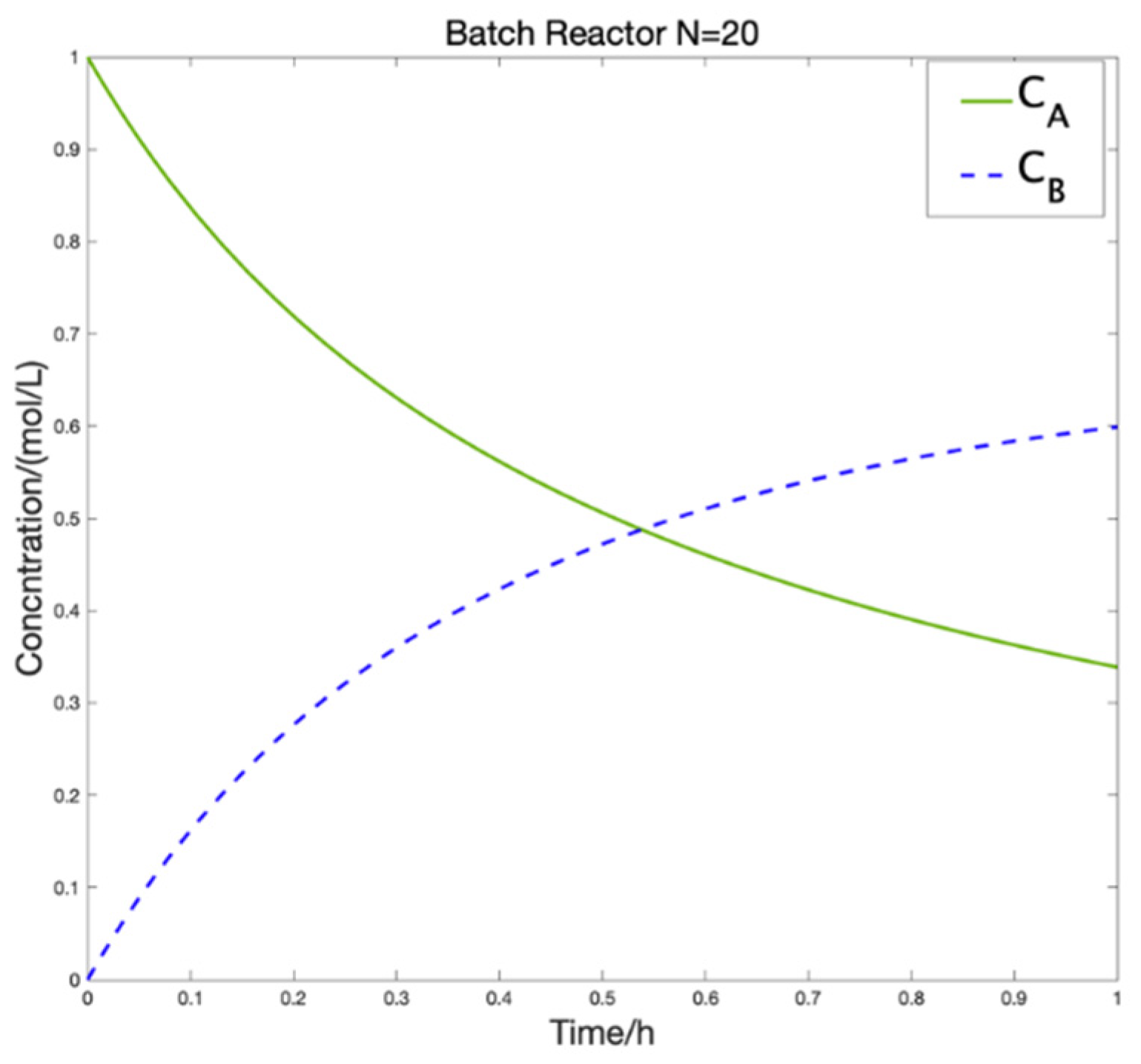
Figure 26.
Optimal temperature control trajectory and iteration curve ().

Figure 27.
Statistical chart of algorithm results.

Figure 28.
Tubular reactor.

Figure 29.
Optimal control trajectory and iteration curve ().

Figure 30.
Optimal control trajectory and iteration curve ().

Figure 31.
Optimal trajectory of state variables ().

Figure 32.
Optimal control trajectory and iteration curve of tubular reactor ().

Figure 33.
Statistical charts of algorithm results.

Figure 34.
Optimal control trajectory and iteration curve ().

Figure 35.
Optimal control trajectory and iteration curve ().

Figure 36.
Optimal control trajectory and iteration curve ().

Figure 37.
Optimal trajectory of state variables ().

Figure 38.
Statistical chart of algorithm results.


Table 1.
Benchmark function.
| Benchmark Test Function | Search Interval | Theoretical Value | |
|---|---|---|---|
| Sphere | [−5.12, 5.12] | 0 | |
| Griewank | [–600, 600] | 0 | |
| Rotated Hyper-Ellipsoid | [−65.536, 65.536] | 0 | |
| Sum Squares | [−10, 10] | 0 | |
| Drop-Wave | [−5.12, 5.12] | −1 | |
| Ackley | [−32.768, 32.768] | 0 | |
| Schaffer n.2 | [−100, 100] | 0 | |
| Sum of Different Powers | [−1, 1] | 0 | |
| Easom | [−100, 100] | −1 | |
| Rastrigin | [−5.12, 5.12] | 0 | |
Table 2.
Experimental results of 5 algorithms.
| Test Function | Algorithm | Best Value | Worst Value | Average Value |
|---|---|---|---|---|
| PSO | 3.4405 × 10⁻⁹ | 1.5306 × 10⁻⁷ | 2.1727 × 10⁻⁸ | |
| BAS | 5.0383 × 10⁻⁶ | 1.7522 × 10⁻⁵ | 6.1773 × 10⁻⁶ | |
| WOA | 1.5911 × 10⁻²² | 8.3121 × 10⁻²¹ | 6.6598 × 10⁻²² | |
| ALO | 7.1305 × 10⁻¹⁵ | 3.8143 × 10⁻¹³ | 5.2281 × 10⁻¹⁴ | |
| HBSO | 0 | 9.3428 × 10−201 | 1.5928 × 10−204 | |
| PSO | 0.0074 | 0.0298 | 0.0123 | |
| BAS | 1.7232 × 10⁻⁶ | 1.1102 × 10⁻⁵ | 5.3476 × 10⁻⁶ | |
| WOA | 1.0814 × 10⁻² | 3.4762 × 10⁻¹ | 1.8842 × 10⁻¹ | |
| ALO | 8.2277 × 10⁻² | 2.9041 × 10⁻¹ | 1.0327 × 10⁻¹ | |
| HBSO | 0 | 0 | 0 | |
| PSO | 1.7935 × 10⁻⁷ | 9.5516 × 10⁻⁵ | 5.6821 × 10⁻⁶ | |
| BAS | 1.0297 × 10⁻⁷ | 2.0875 × 10⁻⁵ | 1.8439 × 10⁻⁶ | |
| WOA | 1.1697 × 10⁻²² | 5.5903 × 10⁻¹⁵ | 6.7422 × 10⁻²¹ | |
| ALO | 3.2245 × 10⁻¹² | 5.8248 × 10⁻¹⁰ | 9.3217 × 10⁻¹¹ | |
| HBSO | 0 | 3.7692 × 10−198 | 9.2261 × 10−201 | |
| PSO | 1.5277 × 10⁻⁹ | 3.5208 × 10⁻⁷ | 1.5627 × 10⁻⁸ | |
| BAS | 9.2061 × 10⁻⁷ | 1.8449 × 10⁻⁵ | 4.3599 × 10⁻⁶ | |
| WOA | 5.6546 × 10⁻²¹ | 1.9977 × 10⁻¹⁹ | 1.0534 × 10⁻²⁰ | |
| ALO | 6.6134 × 10⁻¹³ | 1.9892 × 10⁻¹¹ | 2.3597 × 10⁻¹² | |
| HBSO | 7.1755 × 10−200 | 1.3631 × 10−199 | 9.3572 × 10−200 | |
| PSO | −1 | −0.9962 | −0.9999 | |
| BAS | −0.9323 | −0.5747 | −0.8824 | |
| WOA | −0.9362 | −0.9362 | −0.9362 | |
| ALO | −1 | −0.9362 | −0.9809 | |
| HBSO | −1 | −1 | −1 | |
| PSO | 4.2921 × 10⁻⁴ | 2.3037 × 10⁻¹ | 2.0335 × 10⁻³ | |
| BAS | 5.0334 × 10⁻³ | 3.5262 × 10⁻² | 2.1812 × 10⁻² | |
| WOA | 4.8258 × 10⁻¹⁰ | 1.8859 × 10⁻⁷ | 1.3449 × 10⁻⁹ | |
| ALO | 1.1114 × 10⁻⁶ | 1.3602 × 10⁻⁵ | 8.4639 × 10⁻⁵ | |
| HBSO | 8.8818 × 10⁻¹⁶ | 4.4409 × 10⁻¹⁵ | 9.3579 × 10⁻¹⁶ | |
| PSO | 3.1446 × 10⁻⁹ | 1.3792 × 10⁻⁸ | 9.3415 × 10⁻⁹ | |
| BAS | 1.2486 × 10⁻⁹ | 6.6837 × 10⁻³ | 2.0355 × 10⁻⁵ | |
| WOA | 1.1775 × 10⁻⁴ | 3.0943 × 10⁻³ | 4.6371 × 10⁻⁴ | |
| ALO | 1.3589 × 10⁻¹⁵ | 2.1957 × 10⁻¹³ | 1.5957 × 10⁻¹⁴ | |
| HBSO | 0 | 0 | 0 | |
| PSO | 1.3672 × 10⁻¹³ | 6.5523 × 10⁻⁹ | 9.0066 × 10⁻¹¹ | |
| BAS | 2.0241 × 10⁻⁶ | 9.1889 × 10⁻⁵ | 4.3081 × 10⁻⁶ | |
| WOA | 3.0748 × 10⁻³³ | 6.6872 × 10⁻²⁶ | 5.8416 × 10⁻³⁰ | |
| ALO | 3.0309 × 10⁻¹² | 9.3178 × 10⁻⁹ | 1.6180 × 10⁻¹¹ | |
| HBSO | 1.1078 × 10−205 | 2.5512 × 10−204 | 4.8596 × 10−205 | |
| PSO | −1 | −1 | −1 | |
| BAS | −1 | −0.9997 | −0.9999 | |
| WOA | −0.9999 | −0.9984 | −0.9993 | |
| ALO | −0.9999 | −0.9999 | −0.9999 | |
| HBSO | −1 | −1 | −1 | |
| PSO | 4.1513 × 10⁻⁷ | 1.2533 × 10⁻⁴ | 1.4602 × 10⁻⁶ | |
| BAS | 0.9980 | 7.5814 | 3.9862 | |
| WOA | 7.1054 × 10⁻¹⁵ | 1.9996 | 3.0965 × 10⁻⁹ | |
| ALO | 1.9899 | 4.9748 | 2.9848 | |
| HBSO | 0 | 0 | 0 |
Table 3.
Experimental parameter setting.
| Parameter | Represent | Value |
|---|---|---|
| Beetle population | 50 | |
| Spatial dimension | 20 | |
| The maximum number of iterations | 100 | |
| Correlation coefficient of spiral shape | 0.0001 | |
| The distance between the two antennae | 1 | |
| Beetle step size | 1 | |
| Beetle step size decreasing factor | 0.95 |
Table 4.
Comparison of methods of Case 1.
| Comparison of Other Segment Points | ||
|---|---|---|
| Methods | Segments | Optimum |
| Reference [25] | 4 | 0.76238 |
| EBSO | 10 | 0.76240714 |
| EBSO | 20 | 0.76188931 |
| EBSO | 40 | 0.76135774 |
| IWO-CVP [26] | 50 | 0.76159793 |
| ADIWO-CVP [26] | 50 | 0.76159417 |
| EBSO | 50 | 0.76238 |
| ACO-CP [25] | - | 0.761594156 |
| OCT [27] | - | 0.761594156 |
| IACO-CVP [28] | - | 0.76160 |
| IGA-CVP [29] | - | 0.761595 |
Table 5.
Comparison of methods of batch reactor ().
| Methods | |
|---|---|
| SACA [12] | 0.6100 |
| IKEA [15] | 0.6101 |
| IKBCA [31] | 0.6101 |
| VSACS [32] | 0.6101 |
| Reference [33] | 0.610 |
| IACA [34] | 0.6100 |
| MOARA [35] | 0.60988 |
| AEPF [36] | 0.610070 |
| This work (EBSO) | 0.610558922 |
Table 6.
Comparison of methods of batch reactor ().
| Methods | |
|---|---|
| SACA [12] | 0.6104 |
| IKEA [15] | 0.610426 |
| IKBCA [31] | 0.610454 |
| VSACS [32] | 0.610454 |
| IACA [34] | 0.6104 |
| AEPF [36] | 0.610453 |
| This work (EBSO) | 0.61064758 |
Table 7.
Comparison of methods of batch reactor.
| Comparison of Other Segment Points | ||
|---|---|---|
| Methods | Segments | |
| Reference [25] | 4 | 0.61045 |
| EBSO | 4 | 0.61047235 |
| PSO-CVP [8] | 25 | 0.6105359 |
| AEPF [36] | 25 | 0.610535 |
| EBSO | 25 | 0.61055712 |
| AEPE [36] | 50 | 0.610708 |
| Reference [37] | 50 | 0.6107 |
| EBSO | 50 | 0.61071215 |
| CVP-DE [30] | 60 | 0.6173 |
| EBSO | 60 | 0.61744916 |
| AEPF [36] | 80 | 0.610775 |
| EBSO | 80 | 0.61078114 |
Table 8.
Comparison of methods of tubular reactor ().
| Methods | |
|---|---|
| IKEA [15] | 0.475 |
| VSACS [32] | 0.473630 |
| ndCVP-HGPSO [39] | 0.47363 |
| STA [40] | 0.47363 |
| GA [40] | 0.47363 |
| PSO [40] | 0.47363 |
| This work (EBSO) | 0.47502183 |
Table 9.
Comparison of methods of tubular reactor ().
| Methods | |
|---|---|
| PWV-CVP [3] | 0.4752719 |
| IKEA [15] | 0.4757 |
| IKBCA [31] | 0.4753 |
| VSACS [32] | 0.475272 |
| AEPF [36] | 0.475272 |
| ndCVP-HGPSO [39] | 0.47527 |
| DE [41] | 0.475269 |
| TDE [41] | 0.475269 |
| This work (EBSO) | 0.47627191 |
Table 10.
Comparison of methods of tubular reactor.
| Comparison of Other Segment Points | ||
|---|---|---|
| Methods | Segments | |
| ndCVP-HGPSO [39] | 5 | 0.47260 |
| STA [40] | 5 | 0.47260 |
| GA [40] | 5 | 0.47260 |
| PSO [40] | 5 | 0.47260 |
| EBSO | 5 | 0.47426117 |
| UD-CVP [3] | 15 | 0.47363 |
| PWV-CVP [3] | 15 | 0.47363 |
| ndCVP-HGPSO [39] | 15 | 0.47363 |
| STA [40] | 15 | 0.47453 |
| GA [40] | 15 | 0.47453 |
| PSO [40] | 15 | 0.47453 |
| EBSO | 15 | 0.46011742 |
| AEPF [36] | 40 | 0.476946 |
| DE [41] | 40 | 0.476827 |
| TDE [41] | 40 | 0.476826 |
| EBSO | 40 | 0.47697288 |
Table 11.
Comparison of methods of parallel reaction problem of isothermal tubular reactor.
| Comparison of Other Segment Points | ||
|---|---|---|
| Methods | Segments | |
| Reference [25] | 4 | 0.57284 |
| EBSO | 4 | 0.57296913 |
| AEPF [36] | 10 | 0.572241 |
| EBSO | 10 | 0.57317785 |
| AEPF [36] | 20 | 0.57330 |
| EBSO | 20 | 0.57342901 |
| AEPF [36] | 40 | 0.57348 |
| Equal Division (ISOA) [19] | 40 | 0.573073 |
| Unequal Division (ISOA) [19] | 40 | 0.573535 |
| EBSO | 40 | 0.57412271 |
| AEPF [36] | 80 | 0.57353 |
| CP-APSO [42] | - | 0.573544 |
| CP-PSO [42] | - | 0.573543 |
| Reference [43] | - | 0.5738 |
| CVP [44] | - | 0.56910 |
| CVI [44] | - | 0.57322 |
| Reference [45] | - | 0.57353 |
| MCB [46] | - | 0.57353 |
| CPT [47] | - | 0.57353 |
Publisher’s Note: MDPI stays neutral with regard to jurisdictional claims in published maps and institutional affiliations. |
© 2022 by the authors. Licensee MDPI, Basel, Switzerland. This article is an open access article distributed under the terms and conditions of the Creative Commons Attribution (CC BY) license (https://creativecommons.org/licenses/by/4.0/).
Share and Cite
MDPI and ACS Style
Lyu, Y.; Mo, Y.; Lu, Y.; Liu, R. Enhanced Beetle Antennae Algorithm for Chemical Dynamic Optimization Problems’ Non-Fixed Points Discrete Solution. Processes 2022, 10, 148. https://doi.org/10.3390/pr10010148
AMA Style
Lyu Y, Mo Y, Lu Y, Liu R. Enhanced Beetle Antennae Algorithm for Chemical Dynamic Optimization Problems’ Non-Fixed Points Discrete Solution. Processes. 2022; 10(1):148. https://doi.org/10.3390/pr10010148
Chicago/Turabian StyleLyu, Yucheng, Yuanbin Mo, Yanyue Lu, and Rui Liu. 2022. "Enhanced Beetle Antennae Algorithm for Chemical Dynamic Optimization Problems’ Non-Fixed Points Discrete Solution" Processes 10, no. 1: 148. https://doi.org/10.3390/pr10010148
Note that from the first issue of 2016, this journal uses article numbers instead of page numbers. See further details here.