CFD Modelling of the Fuel Reactor of a Chemical Loping Combustion Plant to Be Used with Biomethane

Abstract

To realize a carbon negative power production technology, it is interesting the option of coupling a Chemical Loping Combustor to a gas turbine. The development of this technology foreseen in the project GTCLC-NEG has some technical barriers, the most important of which is the operation of the chemical looping combustor at high temperature and high pressure conditions. To overcome these limits CFD modeling can be performed to optimize the behavior of the combustor and its design process. This work models the FUEL reactor of a chemical looping combustion plant working in batch mode and based on the reactor available at the Instituto de Carboquimica in Zaragoza, Spain. It is used an oxygen carrier mainly based on 60% mass Fe₂O₃ and 40% mass Al₂O₃. Biomethane is fed to the bottom of the fluidized bed with different velocities and mass flows and the composition of the gases at the outlet of the fuel reactor is measured. The results show that it is possible to model a 2 min duration reduction cycle by running the model for a time comprised between a minimum of 4 h and a maximum of 2 days of simulation. Another important result is the modeling of the chemical reactions happening in the reactor. Kinetics is modelled based on Activation energy (66 kJ/mol) and Pre-exponential factor (4.34 × 10¹ m³ⁿ mol⁻ⁿ s⁻¹). The simple kinetic scheme gives reasonable first approximations and can be used to determine the duration of the reaction, the composition of the exhaust gases and the biofuel conversion.

1. Introduction

The Power Sector is undergoing a rapid technological change with respect to implementation of low carbon technologies. The IEA Energy Outlook [1] shows that the investments in Renewables for the first time are equal to those on the fossil sources. It is likely that the conventional gas turbines and internal combustion engines will need to be integrated in systems employing biofuels and/or CCUS (Carbon Capture Usage and Storage). In addition, the European Union is moving rapidly towards low carbon technologies (i.e., Energy Efficiency, Smart Grids, Renewables and CCUS), see the Energy Union Strategy [2].

In this context a Marie Curie project has been funded in the Spanish National Research Council (CSIC), Instituto de Carboquimica (ICB) named GTCLC-NEG which objective is to promote a Carbon Negative Technology, able to burn multiple biofuels derived from biomass (e.g., pyrolysis oil, biogas and syngas) and to capture the CO₂ emissions at a very low cost. In this way there will be negative GHG emissions, due to the use of BECCS (Bioenergy with Carbon Capture and Storage), a technology which is going to play an important role in the design of future energy systems, according to IPCC scenarios [3].

One of the most critical aspects of the technology is the operation of the Chemical Looping Combustor at high pressures. This has been rarely carried out on the large scale, for this reason the modeling of the reactor and of the chemical reactions that happen during pressurized chemical looping combustion appears to be of scientific interest [4].

Effective models have been already developed at 0D level in the Instituto de Carboquimica [5], these are based on the Shrinking Core Model (SCM) which is widely adopted in literature to describe the oxygen carrier behavior. In addition, CFD models have been developed by [6,7,8,9,10,11,12,13,14,15,16,17,18,19,20,21,22,23,24,25,26,27,28,29]. Nevertheless, the effect of pressure on the CLC process has not yet been fully described and experimented at pilot and industrial scale.

Advancement on CFD Models on Chemical Looping Combustion

A recent review on CFD modeling of fluidized beds further underlines the complexity of this field [30]. This paper aims at presenting an innovative and simple approach, respect to the different strategies which can be found in the literature, to model the fuel reactor with CFD software with improved kinetic constants. The main research groups working on CFD modeling of Chemical Looping Combustion are cited in

Table 1. Most significant works on CFD modeling of Chemical Looping Combustion, Gasification and Reforming.

Group	Source	Software	DEM
Leeds Uni, IFP Energies Nouvelles and Total	[6]	ANSYS FLUENT and EDEM	Yes
Singapore NUS	[7]	N.R.	No
HUST, China	[8]	CPFD	No
Nanjing	[9]	ANSYS FLUENT	No
SINTEF	[10]	PFC3D	Yes
Washington University	[11]	ANSYS FLUENT	Yes
Masdar Institute of Science and Technology	[12]	ANSYS FLUENT	No
TU Darmstadt	[13]	ANSYS FLUENT	No
Imperial College	[14]	ANSYS FLUENT	No
NETL	[15]	Barracuda	No
University of New South Wales	[16]	ANSYS FLUENT	No
Harriot Watt University	[17]	MFIX	No
CPFD Software	[18]	Barracuda-VRTM	No
Indian Institute of Technology	[19]	ANSYS FLUENT	No
The University of Nottingham	[20]	ANSYS FLUENT	No
The University of Newcastle (Australia)	[21]	ANSYS FLUENT	Yes
Harbin Institute of Technology	[22]	K-FIX	No
Zhejiang University	[23]	MFIX	No
University of Utah	[24]	Barracuda-VRTM	No
IMFT Tolouse, TU Wien	[25]	NEPTUNE_CFD	No
The University of Western Ontario	[26]	Barracuda-VRTM	No
KAIST	[27]	ANSYS FLUENT	No
University of North Dakota	[28]	MFIX	No

.

In [6] a CFD-DEM model is realized to study the particles motion inside a cyclone and their interaction with the walls. This is a particularly important theme if inserted in the GTCLC project framework, where cyclones need to have very high efficiency to avoid particles entrainment in the flow of exhaust gases exiting the air reactor. In this model particular attention is also given to attrition, which is another factor which can contribute to the generation of fine dispersed metal particles in the treated gases. In [7] a CFD model is presented in which also chemical reactions are integrated, describing biomass pyrolysis (primary and secondary reactions), char gasification, water-gas shift and metal oxide reduction. Biomass thermal behavior when used in a CLC process, is also important for the GTCLC-NEG project, but in the case of this specific paper it was decided to deal with biomethane to simplify the reaction scheme and calibrate the model with previous experiments performed on CH₄ Chemical Looping Combustion. The work of [8] uses the software CPFD to model an entire CLC plant, comprehending both: the fuel reactor and the air reactor and working with coal. The validation of the model is performed using the pressure sensors of the plant. The model is used to optimize the fuel reactor operation, but limited validation is performed comparing model results with the analysis of exhaust gases produced from the reduction process. Contrary to what is done in [8], in this paper the validation is based on the comparison of the concentrations (in mass and volume) of the gases exiting the fuel reactor. This is due to the interest they have, in particular because they can be used to calculate fuel conversion and carbon dioxide production yields. In the work of [9] both the hydrodynamics and the chemical reactions of the fluidized bed are taken into account. The hydrodynamics it is modelled with the energy-minimization multi-scale (EMMS/matrix) model. Furthermore, heat exchange between the gaseous and the solid phase is taken into account. The validation in this case focuses the attention on the voidage, on the temperature profile and on the gaseous products concentrations measured in the riser (which is the vertical part of the reactor). In the work of [10] a 3D CFD-DEM is used to optimize the design of packed bed reactors. The validation of the complex CFD model has been carried out referring mainly to empirical equations. Banerjee et al. [11] mainly worked on another CFD/DEM model applied to coal chemical looping combustion. In this work the chemical reactions are treated in detail recurring to a complete kinetic scheme of the combustion reactions. In this case the kinetic scheme, is derived from the work of [31]. In this last work the aspect of validation seems less important. In the work of [12] attention is focused on bubble hydrodynamics and diameter. In this model turbulence is simulated based on the k-epsilon turbulence model. The approach to treat the multiphase model is similar to the one adopted also in this work and is based on an Eulerian approach. Same approach is the one adopted also by [13]. The work of Kruggel-Emdem et al. [14] presents a complex CFD model implemented in ANSYS FLUENT^TM which takes into consideration the chemical reactions which happen to the oxygen carrier and models them with a reduced number of reactions which constants are mainly taken from literature. In their work Breault et al. [15] present a CFD model realized in the software Barracuda, which is based on the method called multiphase particle-in-cell (MP-PIC). This is an approach to model particle behavior which is completely similar to the so-called Eulerian-Lagrangian approach. The validation of the model is performed using the data derived from a 50 kWth plant and in particular methane conversion efficiency is taken as one of the key parameters to validate the model.

The work of [16] presents a 3D Euler-Euler model of a coal burning facility. The model is based on a Two-Fluid approach using the standard kinetic theory of granular flow. In another work of the Hariot Watt University [17] the fuel reactor is first modelled with a MFIX CFD software (which is the same as that used in this work) and then the knowledge gained with the CFD simulation is used to control the whole CLC plant model, performed in ASPEN. As said the approach is similar to what will be implemented in the GTCLC-NEG Marie Curie project, managed by ICB-CSIC. The difference between the work performed at Herriot Watt University and the current work is that the type of catalyst is used in ref. [17] is mainly represented by Nickel, while in this work we use iron adsorbed in alumina. The reaction of methane with iron can be considered more simple that that of methane with nickel, because in the first case methane reforming can be neglected.

In the work of Parker et al. [17] the software Barracuda is also used to model a chemical looping combustion system. The entire plant mesh is constituted by 166,000 cells and the simulation is developed in transient conditions and models a period of the length of about 50 s. Barracuda, as said before is a modeling software which is based on a Euler-Lagrangian approach. It was designed to analyse multiphase problems where the fluid phase and the particles phase are encountered. The scale of Barracuda models is more often industrial, while this work is mainly focused instead on lab scale equipment. Barracuda VR is based on the CPFD (Computational Particle Fluid Dynamic) method. The advantages of Barracuda software are the following:

-

it is capable to model full particle size distribution (PSD) for all the solid species;

-

it offers the possibility to model any solid load, from very diluted to packed (i.e., higher than 60% concentration in volume);

-

can perform complete Lagrangian calculations for the solids, the mass, momentum, heat transfer and wear;

-

it has the possibility to model systems with more than 1E16 particles;

-

it can perform calculation of chemical reactions, specifically for each particle it provides highly accurate results, because they are dependent from the composition, temperature and size of each particle.

Menon et al. [19] present in their work a 2D model realized in ANSYS FLUENT^TM (Canonsburg, PA, USA), simulating a fuel reactor fed with coal. The reaction scheme is mainly taken from literature and the model implemented is based on Euler-Euler approach. Chen et al. [20] in their work present a 3D model of the fuel reactor. The approach is always Elulerian-Eulerian (i.e., the two fluids model). The equations are closed with the kinetic theory of granular flow (KTGF). The chemical kinetic model is based on TGA experiments mainly performed at the Instituto de Carboquimica in Zaragoza, Spain [32,33,34]. The kinetic parameter determination is based on the shrinking core model (SCM), as also reported in refs. [5,32,35]. The oxygen carriers taken into account are mainly cu-based. In [21] the authors perform a CFD-DEM study of the circulation rate. In this way assuming cold flow CFD software can be used to optimize the circulation rate of the reactor and so to optimize its design parameters. Shuai et al. [22] simulate the hydrodynamics and also chemical reaction kinetics of a fuel reactor using k-FIX, which is a precursor of MFIX software, choosing the total variation diminishing method (TVD) scheme to solve the equations. The work of [23] assumes a particularly interesting meaning, if compare with the work presented in this paper, because it shows which could be the future developments, after the simulation and optimization of the batch fuel reactor. Continuous process in fact will have to be studied. In this case a whole plant comprising of FUEL reactor and air reactor is modelled using MFIX software. The approach adopted is Euler-Euler (i.e., two fluids). The validation of the model is based on the concentration of the gases exiting the reactors, this is a similar approach to the one adopted in this paper. Chemical reactions are also modelled and it is used a kinetic triplet available in the literature. Reinking et al. [24] in their model use again Barracuda^TM (CPFD Software Sulzer Pumps USA, Houston, TX, USA) to simulate a continuous industrial plant. No significant differences exist with respect to the already presented works. The work of Hamidouche et al. [25] presents a comparison between 0D and 2D models. In [26] again Barracuda^TM software (CPFD Software Sulzer Pumps USA, Houston, TX, USA) is used to model a plant at industrial scale. The length of the time period which is modelled is about 60 s. In [27] a model realized in FLUENT is presented and it is solved with Phase-Coupled SIMPLE (PC-SIMPLE) algorithm that is applied for the pressure-velocity coupling and correction. Finally in [28] a spouted bed reactor is studied. It is modeled with a Eulerian-Eulerian approach, based on the twin fluid model implemented in MFIX software. The parameters investigated to understand their influence on the reactor behavior were the following: bed height, draft tube height from the bottom, draft tube internal diameter, spout diameter, spout velocity, background velocity. Where the draft tube is a tube inserted in the middle of the reactor to grant the generation of the spout.

2. Materials and Methods

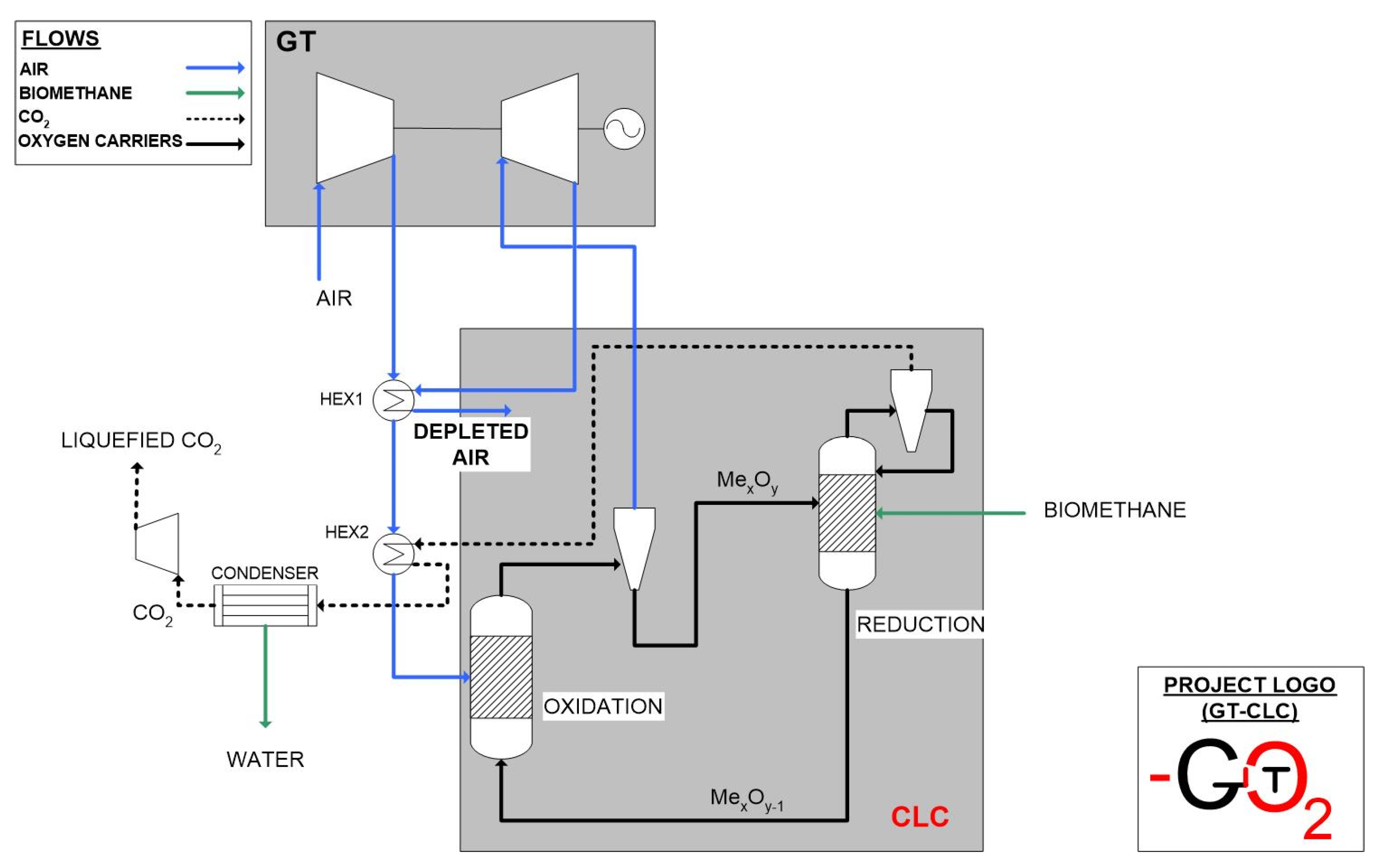
2.1. GTCLC-NEG Plant Description

The proposed plant is based on the coupling of a Chemical Looping Combustor to a gas turbine, as reported in Figure 1.

As it can be seen in the proposed plant the compressed air used to oxidize the oxygen carrier in the air reactor is then expanded in a gas turbine to produce electricity. In the fuel reactor biofuels (in this case biomethane) are used to reduce the oxygen carrier. Possible technical barriers of the proposed plant are the following: (1) oxygen carriers with high oxygen transport capacity are needed; (2) low attrition rate oxygen carriers are needed, which can work in extreme conditions; (3) kinetics aspects under high pressure and temperature conditions are not known; (4) reactor injection system has to be adapted to different types of biofuels (gaseous, liquid and solid biofuels); (5) the use of the hot air produced from the air reactor (see Figure 1) in a gas turbine has to be optimized; (6) exhausts should be filtered to retain the dust released by oxygen carrier attrition; (7) high electrical efficiency of the power system has to be granted and (8) high fuel conversion in the combustor has to be achieved [35,36,37].

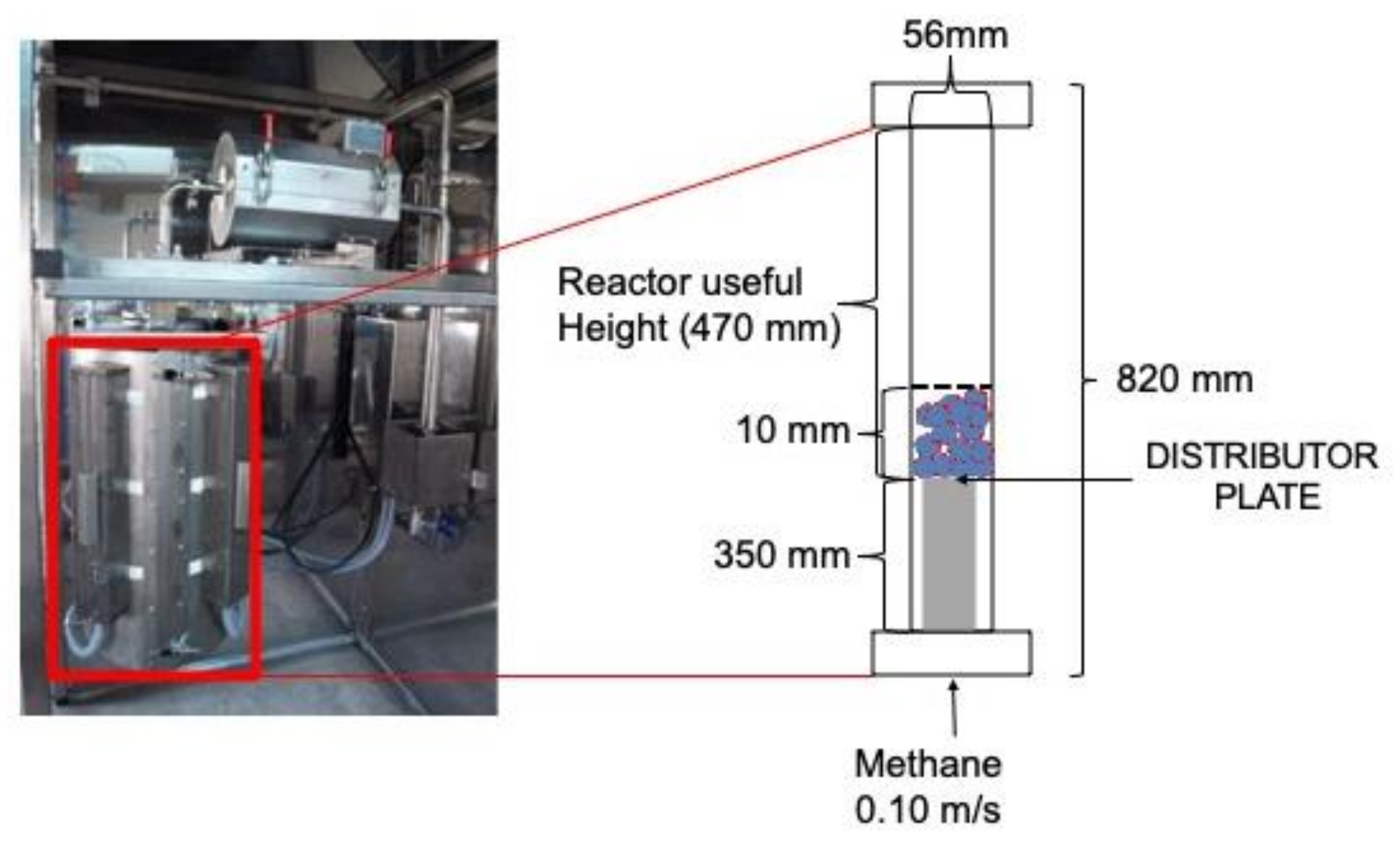
2.2. Batch Reactor Characteristics

The geometric parameters of the reactor are shown in Figure 2. The used oxygen carrier is shown in Figure 3. We see from Figure 2 that for the modeling it is considered only the “active” part of the reactor, which is the one which is right above the gas injection part. This has a diameter of 56 mm and a height of 470 mm. The height of the bed is 10 mm. Another important thing to note is that the inlet of the gas is locate at the bottom of the reactor and together with methane also nitrogen is inserted with a volumetric ratio of 70% nitrogen and 30% methane.

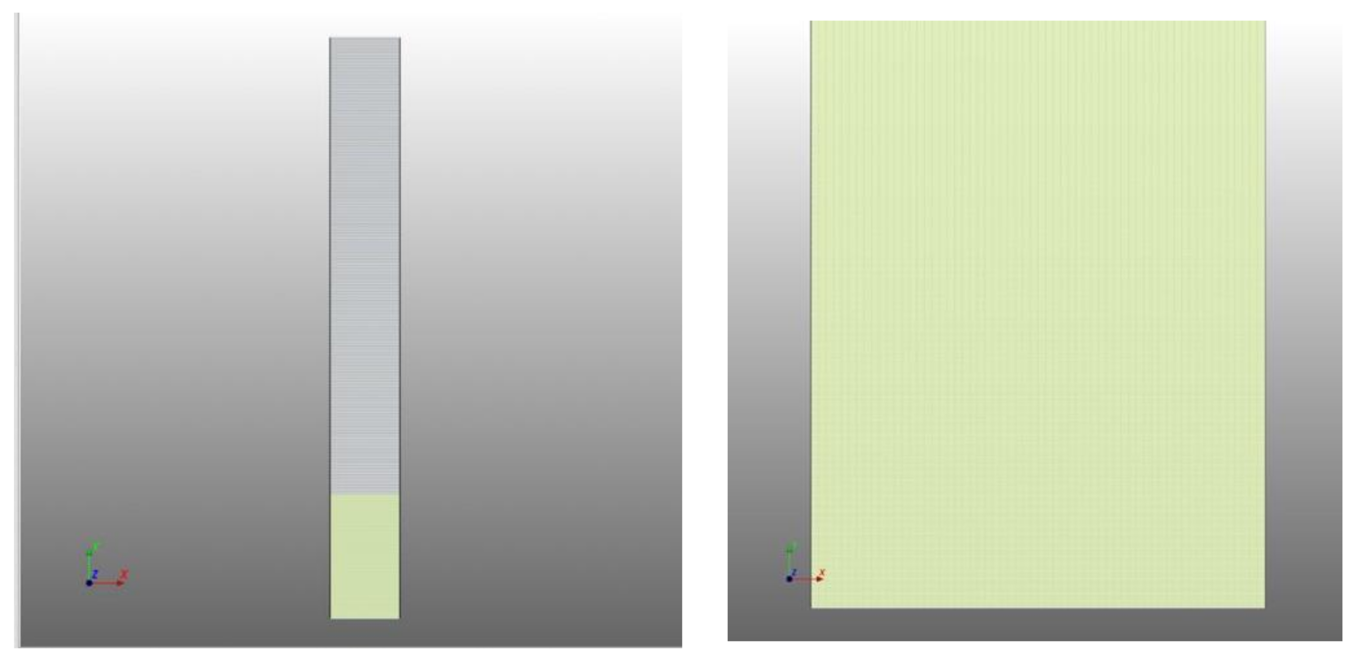
2.3. Mesh Characterization

The mesh is characterized by about 14,000 rectangular cells of the following dimensions:

-

x: 7.00E-4 m

-

y: 2.61E-03 m.

A more refined mesh with 30,000 cells has also been realized, to perform a sensitivity analysis on the influence of the mesh refinement grade on the final results. The Parameters of the two final meshs are proposed in

Table 2. Mesh characteristics.

	Mesh<	Mesh>
Scalar Standard Cells	14,000	30,000
Aspect ratio of scalar standard cells	1	1

.

From Table 2 it can be seen that all the cells are 100% scalar standard cells, which avoid overlapping each other and cutting each other. Furthermore, in both cases the aspect ratio of the cells is equal to 1 (which is the optimal value).

MFiX^® software uses a meshing method different from the common ones. Specifically, it uses the FAVOR (Fractional Area/Volume Method). Which is a full orthogonal meshing method. FAVOR can model complex geometric regions with simplicity. In the case of meshes done in alert zones (i.e., in areas with large geometrical variations, such as areas with curves or very small structures) no trouble appears, due to the fact that when these difficulties appear the created cells are cut, and the centroid is moved to a new position. In Figure 4 the used mesh is shown.

2.4. The CFD Model

Based on the approach which is also shown in the work of Porrazzo et al., 2016 [17], the continuum flow solver in open-source code MFIX 21.2, which is a multi-fluid Eulerian–Eulerian code, with each phase treated as an interpenetrating continuum was used in this study. Mass and momentum conservation equations are solved for the gas and solids (i.e., particulates) phases, with kinetic granular theory providing the appropriate closure relations [38].

In kinetic granular theory, a granular temperature, proportional to the mean square of the random particle velocity based on the Maxwellian velocity distribution, is defined to model the fluctuating energy of the solid phase. Instead of solving a differential equation for granular temperature, an equilibrium between its generation and dissipation is assumed and an algebraic relationship, see Equation (19), is used. Using this simplified algebraic form of the granular temperature equation has negligible effect on numerical results but saves the computational time greatly, compared to solving the full partial differential equation. Constitutive relations for the solids phase stress tensor are based on the kinetic theory [39,40]. For the dense gas–solids flow considered in the current study, turbulence of the gas phase is not of primary concern, as particle–particle collisions dominate the flow, hence at the beginning it was taken the decision to avoid the use of turbulence models. In a second moment it was decided to perform a sensitivity analysis on the k-epsilon model by just comparing the results obtained without k-epsilon with those obtained using the k-epsilon model.

The widely used drag correlation proposed by Gidaspow, 1994 [39] which is a combination of Wen and Yu [41] and Ergun [42] correlations is used to describe the interphase interaction between gas and solids. The main governing equations solved in MFIX 21.2 are summarized in the following paragraph. More details on theory and numerical techniques in MFIX can be found in [43] (see also Benyahia et al., 2012 [44], Syamlal, 1998 [45], Syamlal et al., 1993 [46]). The list of the main equations used in the model is presented as follows and it is taken by [38].

Governing Equations

(a)

Continuity Equations

$$\frac{\partial }{\partial t}\left({\epsilon }_g{\rho }_g\right)+\nabla \left({\epsilon }_g{\rho }_g\overrightarrow{V_g}\right)=0$$

(1)

$$\frac{\partial }{\partial t}\left({\epsilon }_p{\rho }_p\right)+\nabla \left({\epsilon }_p{\rho }_p\overrightarrow{V_p}\right)=0$$

(2)

(b)

Momentum equations

$$\frac{\partial }{\partial t}\left({\epsilon }_g{\rho }_g\overrightarrow{V_g}\right)+\nabla \left({\epsilon }_g{\rho }_g\overrightarrow{V_g}\overrightarrow{V_g}\right)=\nabla {\stackrel{=}{\tau }}_g-{\epsilon }_g\nabla P+{\epsilon }_g{\rho }_{g}g-I_{gp}$$

(3)

$$\frac{\partial }{\partial t}\left({\epsilon }_p{\rho }_p\overrightarrow{V_p}\right)+\nabla \left({\epsilon }_p{\rho }_p\overrightarrow{V_p}\overrightarrow{V_p}\right)=\nabla {\stackrel{=}{\tau }}_p-{\epsilon }_p\nabla P+{\epsilon }_p{\rho }_{p}g+I_{gp}$$

(4)

Governing Equations

(a)

Gas stress tensor

$${\stackrel{=}{\tau }}_g=2{\mu }_g{\stackrel{=}{S}}_g$$

(5)

$${\stackrel{=}{S}}_g=\frac{1}{2}\left(\nabla \overrightarrow{V_g}+{\left(\nabla \overrightarrow{V_g}\right)}^T\right)-\frac{1}{3}\nabla \overrightarrow{V_g}\stackrel{=}{I}$$

(6)

(b)

Solid stress tensor

$${\stackrel{=}{\tau }}_p=\left(-P_s+\eta {\mu }_b\nabla \overrightarrow{V_p}\right)\stackrel{=}{I}+2{\mu }_p{\stackrel{=}{S}}_p$$

(7)

$${\stackrel{=}{S}}_p=\frac{1}{2}\left(\nabla \overrightarrow{V_p}+{\left(\nabla \overrightarrow{V_p}\right)}^T\right)-\frac{1}{3}\nabla \overrightarrow{V_p}\stackrel{=}{I}$$

(8)

$$P_s={\epsilon }_p{\rho }_p{\Theta }_p\left(1+4g_0{\epsilon }_p\eta \right)$$

(9)

$${\mu }_p=\left(\frac{2+\alpha }{3}\right)\left[\frac{{\mu }_p^{*}}{g_0\eta \left(2-\eta \right)}\left(1+\frac{8}{5}\eta g_0{\epsilon }_p\right)\left(1+\frac{8}{5}\eta \left(3\eta -2\right)g_0{\epsilon }_p\right)+\frac{3}{5}\eta {\mu }_b\right]$$

(10)

$${\mu }_p^{*}=\frac{{\epsilon }_p{\rho }_p{\Theta }_p{g}_0\mu }{{\epsilon }_p{\rho }_p{\Theta }_p{g}_0+\frac{2\beta \mu }{{\epsilon }_p{\rho }_p}}$$

(11)

$$\mu =\frac{5}{96}{\rho }_p{d}_p\sqrt{\pi {\Theta }_p}$$

(12)

$${\mu }_b=\frac{256}{5\pi }\mu {\epsilon }_{p{g}_0}^2$$

(13)

$$\eta =\frac{1+e}{2}$$

(14)

$${\stackrel{=}{\sigma }}_{p,fric}=-P_{s,fric}\left(\stackrel{=}{I}-\frac{\sin \Phi }{\sqrt{I_{2D}}}{\stackrel{=}{D}}_p\right)$$

(15)

$${\mu }_{fric}=\frac{P_{s,fric}\sin \Phi }{2\sqrt{I_{2D}}}$$

(16)

$$P_{s,fric}=\left\{\begin{array}{c}{10}^{24}{\left({\epsilon }_p-{\epsilon }_p^{*}\right)}^2 {\epsilon }_p>{\epsilon }_p^{*}\\ 0 {\epsilon }_p>{\epsilon }_p^{*} \end{array}\right.$$

(17)

(c)

Granular temperature

$${\Theta }_p={\left[\frac{-\left(K_1{\epsilon }_p+{\rho }_p\right)T_r\left({\stackrel{=}{D}}_p\right)}{2K_4{\epsilon }_p}+\frac{\sqrt{{\left(K_1{\epsilon }_p\right)}^{2}T{r}^2\left({\stackrel{=}{D}}_p\right)+4K_4{\epsilon }_p\left[2K_{3}Tr\left({\stackrel{=}{D}}_p^2\right)+K_{2}T{r}^2\left({\stackrel{=}{D}}_p\right)\right]}}{2K_4{\epsilon }_p}\right]}^2$$

(18)

$$K_1=2\left(1-e\right){\rho }_p{g}_0$$

(19)

$$K_2=\frac{4}{3\sqrt{\pi }}{d}_p{\rho }_p\left(1+e\right)g_0{\epsilon }_p-\frac{2}{3}{K}_3$$

(20)

$$K_3=\frac{d_p{\rho }_p}{2}\left\{\frac{\sqrt{\pi }}{3\left(3-e\right)}\left[\frac{\left(3e+1\right)}{2}+\frac{2}{5}\left(1+e\right)\left(3e-1\right)g_0{\epsilon }_p\right]+\frac{8{\epsilon }_p}{5\sqrt{\pi }}{g}_0\left(1+e\right)\right\}$$

(21)

$$K_4=\frac{12\left(1-e^2\right){\rho }_g{g}_0}{d_p\sqrt{\pi }}$$

(22)

$$g_0=\frac{1-0.5{\epsilon }_p}{{\left(1-{\epsilon }_p\right)}^3}$$

(23)

(d)

Inter-phase momentum exchange

$$I_{gp}=\beta \left({\overrightarrow{V}}_g-{\overrightarrow{V}}_p\right)$$

(24)

$$\beta =\left\{\begin{array}{c}150\frac{{\epsilon }_p^2{\mu }_g}{{\epsilon }_g{d}_p^2}+1.75\frac{{\epsilon }_p{\rho }_g\left|{\overrightarrow{V}}_p-{\overrightarrow{V}}_g\right|}{d_p} if {\epsilon }_p>0.2\\ \frac{3}{4}{C}_d{\epsilon }_g-2.65\frac{{\epsilon }_p{\epsilon }_g{\rho }_g\left|{\overrightarrow{V}}_p-{\overrightarrow{V}}_g\right|}{d_p} if {\epsilon }_p \leqq 0.2\end{array}\right.$$

(25)

$$C_d=\left\{\begin{array}{c}\frac{24}{Re·{\epsilon }_g}\left(1+0.15{\left(Re·{\epsilon }_g\right)}^{0.687}\right)\\ 0.44 if Re·{\epsilon }_g\geqq 1000\end{array}\right.if Re·{\epsilon }_g<1000$$

(26)

$$Re=\frac{{\rho }_g\left|{\overrightarrow{V}}_p-{\overrightarrow{V}}_g\right|d_p}{{\mu }_g}$$

(27)

In particular, the list of equations above, indicates the most important phenomena which regulate the hydrodynamic aspects, but also heat transfer processes have to be considered and also:

-

the conservation of internal energy;

-

the conservation of granular energy;

-

the boundary conditions (with particular attention to the wall heat transfer phenomena).

For a detailed analysis of these phenomena the following document has to be considered: [46].

2.5. The Modeling Platform

The modeling platform is shown in Figure 5 and it is based on the MFIX 21.2 code developed by NETL.

The 2D model implemented in MFIX 21.2 code is based on the Eulerian–Eulerian approach. Gas and solid phases are considered as continuum phases in the domain under investigation. The solid phase is characterized by uniform spherical particles of constant mean density and diameter. Continuity and momentum equations in two directions (x and y) are solved for both phases and the exchange of mass and momentum between them is taken into account. If the hydrodynamic model of the reactor is modeled with MFIX 21.2 software (NETL US DOE, Houston, TX, USA), the kinetic part is simulated with a User Defined Function (UDF) specifically determined from the model developed by Cabello et al., 2014 [47]. The modeled oxygen carrier is prepared by impregnation of iron on alumina and the kinetic is determined in a TGA by modeling particle reaction through the Shrinking Core Model (SCM). The the physical properties and the kinetic properties of the oxygen carrier are proposed in Table 2. The oxidation reaction is shown in Equation (1) and the reduction reaction is shown in Equation (29).

$$4. F{e}_3{O}_4+O_2\to 6F{e}_2{O}_3$$

(28)

$$12. F{e}_2{O}_3+C{H}_4\to 8F{e}_3{O}_4+C{O}_2+2H_{2}O$$

(29)

The fuel used is assumed to be biomethane, because the technology to be developed is a carbon negative emissions technology. The results obtained by the simulation are then elaborated in the ParaView (Sandia National Laboratories, Kitware Inc., Los Alamos National Laboratory, Los Alamos, NM, USA) Environment, which is open source. Both ParaView and MFIX 21.2 are operated in Linux. This gives the possibility to access with more detail the codes of MFIX 21.2, which GUI is coded in python while the model is coded in Fortran. The simulations will also use the computational cluster of CSIC TRUENO, which is equipped with 16 processors, has 64 GB RAM of memory and works with OPEN-MPI parallelization.

2.6. The Modeling Conditions

Oxygen carrier properties are shown in

Table 3. Oxygen carrier properties [47].

Parameter	Value	Unit of Measure
Oxygen carrier	Fe2O3	-
Promoting Support	Al2O3	-
Total Fe2O3 content 1	20	wt%
Average Particle size	200–400	μm
Particle density	3950	kgm−3
Porosity	50.5	%
BET	39.1	m2/g
Order of reaction	0.25	-
Pre-exponential factor kinetics	4.34 × 101	m3nmol−ns−1
Activation energy kinetics	66	kJ/mol
Oder of diffusion	-	0
Pre-exponential factor diffusion	9.80 × 1030	m3nmol−ns−1
Activation energy diffusion	672	kJ/mol

¹ Determined by ICP-AES.

, while the modeling conditions are shown in

Table 4. Modeling conditions.

Parameter	Value	Unit of Measure
Temperature	950	°C
P	1	atm
D	56	mm
h	470	mm
u0	0.10	m/s
ε	0.5	-
Bh (bed height)	10	mm
Wall thermal behavior	Adiabatic	-
Grid size	14,000	cells
Solver	Two-fluid model (MFIX-TFM)	-
Drag model	Syamlal-O’Brien	-
C1	0.8	-
D1	2.65	-
Momentum formulation	Model A, See Abanades et al. 1993 [49]	-
UDF	User Defined Function	-
Thermal conductivity of solids	Bauer and Schlünder	-
Diffusivity	Dilute mixture approximation (air)	-
Pressure outlet	“Pressure Outflow”	1.0132e + 05 Pa

. We can see that in Table 3 the support is called “promoting support”, instead of “inert support”. It is believed in fact that alumina is reacting with iron and modifies it to enhance its oxygen transport properties. As reported in ref. [48] alumina could have a role on the formation of oxygen vacancies, which promote the oxygen carrier properties of the adsorbed iron.

The reactor diameter and height have been already presented in Figure 2. The data reported in Table 3 have been measured at the Instituto de Carboquimica, Zaragoza, Spain. For this purpose, different techniques have been adopted. The total iron content has been measured using inductively coupled plasma atomic emission spectroscopy (ICP-AES) with a Jobin Yvon 2000 spectrometer (HORIBA Jobin Yvon, Kyoto, Japan). The mean particle diameter was measured with laser diffraction technique, according to the ISO 13320 using a LS 13320 Beckman Coulter equipment (Beckman Coulter, Pasadena, CA, USA). The skeletal density of the particle was determined with a helium pycnometer Micromeritics Model AccuPyc II 1340 (Micromeritics, Norcross, GA, USA). The crushing strength of the particle was determined with a Shimpo FGN-5X measuring machine (ELECTROMATIC Equip’t Co., Lynbrook, NY, USA). Porosity was measured through Hg intrusion using a Quantachrome Pore-Master 33 instrument (Quantachrome, Boynton Beach, FL, USA). Specific surface of pores was determined instead using a Brunauer-Emmet-Teller (BET) method, through adsorption/desorption in nitrogen at 77 K in a Micrometrics SAP-2020 (Micromeritics Inc., Norcross, GA, USA). Crystalline structure of the oxygen carrier was determined by powder x-ray diffraction (XRD) in a Bruker AXS D8 advance system (Bruker Inc., Billerica, MA, USA). The reducibility of the Fe-based oxygen carrier particles was determined with temperature-programmed reduction (TPR) experiments in an AUTOCHEM II, apparatus produced by Micrometrics (Micromeritics Inc., Norcross, GA, USA). Kinetic parameters have been determined instead in a TGA CI Electronics type, described in [50]. From Table 3 it can be seen that the reactor temperature is set to 950 °C, this is obtained by inserting a hot flow of methane from the bottom of the reactor which heats up all the internal part of the reactor, exchanging heat with the particles of the bed and the produced gases. The heat of the incoming gases is used also to supply the heat needed to perform the reduction reaction. The height of the bed in the reactor is about 10 mm, the wall is supposed to be adiabatic. As already said an initial grid size of 14,000 cells was chosen. Then a sensitivity analysis on grid size was performed working with 30,000 also. The settings used for the MFIX software are quite conventional, the only thing to note is the use of a UDF (User Defined Function) to provide the reaction chemistry.

2.7. The Solver and Convergence Parameters

According to the document “MFIX Documentation Numerical Technique” [45], the transport equation contains convection and diffusion terms which are discretized using second order accurate discretization schemes. These are mainly based on the “universal limiter” as proposed by [51].

The two equations of diffusion and convection represent the transient terms, these two differential equations are used to produce an algebraic equation, which is integrated over a control volume. The parameters for discretization are shown in the numerics section of the software, see

Table 5. Discretization parameters.

Temporal Discretization	Implicit Euler	-
Spatial discretization
Scheme		Relaxation factor
Gas pressure	First-order upwind	0.8
Volume fraction	First-order upwind	0.5
U-momentum	First-order upwind	0.5
V-momentum	First-order upwind	0.5
W-momentum	First-order upwind	0.5
Energy	First-order upwind	1.0
Mass Fraction	First-order upwind	1.0
Granular Energy	First-order upwind	0.5
Scalar/k-ε	First-order upwind	0.8
DES diffusion	First-order upwind	1.0

.

An extension of SIMPLE [52] is used for solving the discretized equations. Several issues need to be addressed when this algorithm, developed for single phase flow, is extended to solve multiphase flow equations. In the work [53] three main issues are listed:

(i) There are more field variables, and hence more equations compared with single phase flow. This slows the computations, but does not in itself make the algorithm any more complex.

(ii) Pressure appears in the three single phase momentum equations, but there is no convenient equation for solving the pressure field. The crux of SIMPLE algorithm is the derivation of such an equation for pressure—the pressure correction equation. The pressure corrections give velocity corrections such that the continuity equation is satisfied exactly (to machine precision). There is no unique way to derive such an equation for multiphase flow, since there is more than one continuity equation in multiphase flow.

(iii) The multiphase momentum equations are strongly coupled through the momentum exchange term. Making this term fully implicit for the success of the numerical scheme is essential. This is the main idea in the Implicit Multifield Field (IMF) technique presented in [54], which is encoded in the K-FIX (Kachina- Fully Implicit Exchange, Los Alamos National Laboratory, Los Alamos, NM, USA) program of [55]. In the MFIX algorithm the momentum equations are solved for the entire computational domain. To make the exchange term implicit all the equations for each velocity component (e.g., u-equations for gas and all solids’ phases) must be solved together, which leads to a nonstandard matrix structure. A cheaper alternative is to use the Partial Elimination Algorithm (PEA) of [53]. The parameters used for the solver are shown in the numerics session. BICGSTAB solver, which stands for, Conjugate Gradient(CG), Bi-Conjugate gradients stabilized (BiCGStab) is used to solve the linear systems, see [56,57] (see

Table 6. Settings for the solver.

Solver		Iterations	Tolerance
Gas pressure	BICGSTAB	20	0.0001
Volume fraction	BICGSTAB	20	0.0001
U-momentum	BICGSTAB	5	0.0001
V-momentum	BICGSTAB	5	0.0001
W-momentum	BICGSTAB	5	0.0001
Energy	BICGSTAB	15	0.0001
Mass fraction	BICGSTAB	15	0.0001
Granular energy	BICGSTAB	15	0.0001
Scalar/κ-ε	BICGSTAB	15	0.0001
DES diffusion	BICGSTAB	10	0.0001

).

The preconditioner parameters are shown in

Table 7. Settings for the preconditioner.

Preconditioner		Sweep
Gas pressure	Line relaxation	Red-black sweep
Volume fraction	Line relaxation	Red-black sweep
U-momentum	Line relaxation	Red-black sweep
V-momentum	Line relaxation	Red-black sweep
W-momentum	Line relaxation	Red-black sweep
Energy	Line relaxation	Red-black sweep
Mass fraction	Line relaxation	Red-black sweep
Granular energy	Line relaxation	Red-black sweep
Scalar/κ-ε	Line relaxation	Red-black sweep
DES diffusion	Line relaxation	Red-black sweep

.

The time step for the iterations of the model is 1.0E-03. The various numerical parameters used to solve the case are reported in the Numerics section. This describes:

-

residuals: these are the criteria used for convergence for each type of equation, as well as the maximum number of iterations and residuals normalization options;

-

discretization: defines temporal, special discretization schemes and relaxation factors for each equation;

-

linear solver: defines the linear equation solver, tolerance and maximum number of iterations for each equation;

-

preconditioner: defines the preconditioner options for each equation;

-

advanced: defines less common parameters, such as the maximum inlet velocity factor, drag and IA theory under-relaxation factors and fourth order interpolation scheme.

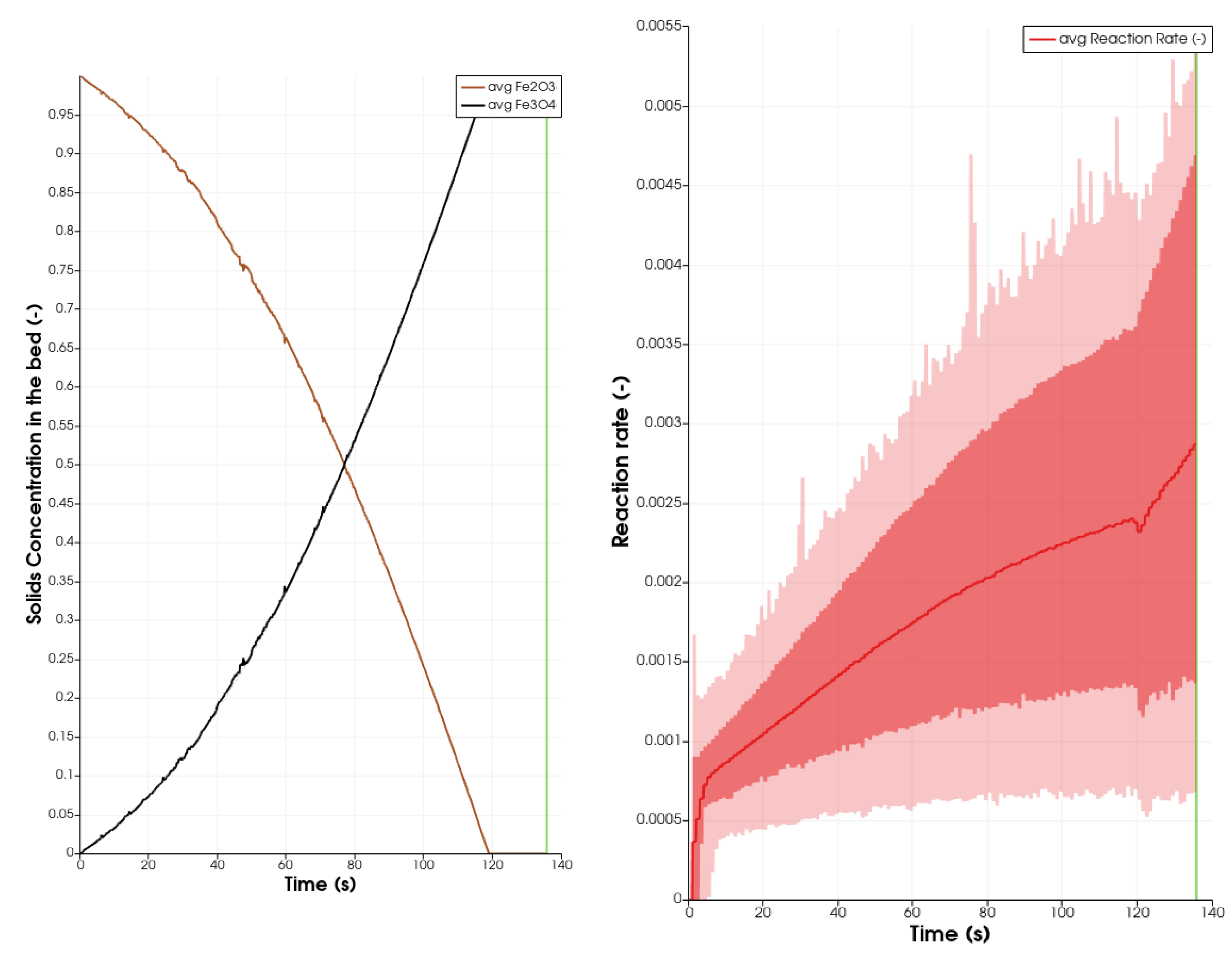
Advanced parameters for the simulation are shown in

Table 8. Advanced setting.

Maximum Inlet-Velocity Factor	1
Dilute threshold	0.0001
Minimum tracked solids volume factor	1E-08
Skip continuing residuals if volume fraction below	1E-07
Drag under-relaxation factor	1.0
IA theory conductivity under-relaxation factor	1.0

. The chosen residuals input values are reported in

Table 9. Residuals input values.

Parameter	Value
Maximum iterations	50
Fluid normalization	0.0
Fluid pressure correction scale factor	10.0
Solids normalization	-
Solids volume fraction correction scale factor	10.0
Maximum residual at convergence Continuity + momentum Energy Species Granular energy Scalar κ-ε	0.001 0.0001 0.0001 0.0001
Maximum residual for divergence	10,000.0

.

3. Results

In Figure 6 it is shown the trend of the gas velocity magnitude. This is the typical value which can be derived also by the 0D or 1D models developed in the group of gasification of the Instituto de Carboquimica, CSIC in Zaragoza.

Trends similar to that produced in Figure 6 can be obtained also with 0D software, such that developed by [5]. In [5] we see for example the representation of the trend of the composition of the gases throughout the reactor which qualitatively confirms the trends shown in this work. In another publication [58], always realized by the group of the Instituto de Carboquimica, we have a clear idea of what is instead the trend of the velocity inside the reactor. The model is applied in that case to a plant of the thermal power of 100 kWth. The reactor, compared to the one which is taken into consideration in this study has a height of 5 m and we see that the value of the velocity goes increasing from a starting value of 1 m/s to a final value of 4 m/s (after touching a peak of 5 m/s). In the results presented in Figure 6 we see that the final values are much lower, but this can depend on the smallest scale of the reactor and reduced height. What we see is that with the CFD software we can measure many oscillations that with 1D models may be not tracked. In both cases a big influence in the flow is exerted by the bed, which fills the reactor and is responsible for the oscillations.

Another 1D model that indicates the trend of the velocity inside the reactor is that shown in [59]. A similar trend of velocities as in [58] is reported. It can also be noted that the velocity is influenced by the gas conversion, which in this case is different between the 2 reactors modelled in [58,59] and this work.

As it can be seen from Figure 7, despite the inlet temperature of the gas is set to 950 °C the fact that the iron and the reactor temperature at the second equal to zero are set at ambient temperature, implies that the average temperature inside the reactor reaches after 120 s an average value of about 750 °C.

In Figure 8 the average numbers of the gas velocity inside the reactor are shown. The data represent the average at each point in time of all the values of velocity which have been calculated in the different cells of the geometrical model.

In Figure 9 it is reported the average volumetric flow inside the reactor. This is calculated based on the average gas velocity inside the reactor, by applying the following script (which has been inserted in ParaView calculator tool, Sandia National Laboratories, Kitware Inc., Los Alamos National Laboratory, Los Alamos, NM, USA):

$$\mathrm{mag}\left(\mathrm{Gas} \mathrm{Velocity}\right)\times \mathrm{D}2\times \mathsf{\pi }/4\times 1000\times 60$$

(30)

the Gas Velocity variable is a vector, for this reason it is required to perform the module of it (see the command “mag”). D is the diameter expressed in meters (the value in millimeters is reported in Table 5). The value is multiplied for 1000 to convert from cubic meters to liters and then it is divided for 60 to convert from seconds to minutes, so the final unit of measure of L/min is obtained.

In Figure 10 the mass fraction of the biomethane through all the surface of the reactor is presented. We can see that the biomethane enters the reactor with a mass fraction of the gas which is high at the beginning, i.e., at the bottom of the reactor, and it is equal to 0.57 (the mass fraction of nitrogen gas is about 0.43). While the gas passes through the fluidized bed it decreases its concentration and progressively is converted into water and carbon dioxide.

The average gas yields during time are reported in Figure 11, they are normalized concentrations, calculated once the concentration of nitrogen is subtracted.

As we have already stated in the introduction exhaust gases composition in the reactor can be an effective way to validate many CFD models, developed on such batch reactors. In this case, the paper [60] presents a set of tests performed with the same catalyst on both batch and continuous reactors. Dealing with the batch reactor this was operated with similar conditions to the ones tested in this CFD model and most of all with the same solid inventory, equal to 55 kg/MW. We can say that the validation proposed in Figure 11 is still qualitative in the sense that in the model the gases are inserted already heated, while in the real case the reactor is heated externally and this makes the two cases comparable only in part. The publication [60] shows that with similar conditions the duration of the conversion process of biomethane into CO₂ and H₂O is in the range of few seconds, the fact that in our case the conversion of the gas lasts much more time can be due to the not perfect control of the heating ramp of the reactor which, as said, is more controlled by the inlet temperature of the gases, than from external electrical heating. This affects the internal temperature of the reactor, which results to be lower than that used in the experiments performed in [60]. On the other hand, once that the reaction happens the composition of the exhaust gases results comparable with that measure during the experiments.

Figure 12 reports the increase in bed height. From the figure we infer that since the first seconds of the simulation we assist to the bed expansion phenomenon, which brings the height to an increase of 1.5 times (the bed height of the reactor before starting the flow of fuel gas was 0.1 m and it becomes during reactor operation about 0.15 m). This is confirmed by several studies, among which [61].

In Figure 13 we show how the concentration of Fe₂O₃ changes during time in the bed of the reactor, this confirms that in 120 s we are able to convert all the bed material to Fe₃O₄ in an efficient way. This figure can be correlated with Figure 10 of this same paper, in which we see that after about 120 the biomethane inserted in the reactor ceases to convert into water and carbon dioxide because the oxygen carrier has reduced its action. Figure 13 explains also the increase in the concentration of biomethane which is noted in Figure 11 and the change in velocity, temperature and volumetric flow which is shown in Figure 7, Figure 8 and Figure 9.

4. Discussion

4.1. Further Validation

To understand well the results of the modeling performed, we can base on the results of the 0D models developed at the Instituto de Carboquimica in Zaragoza, Spain. In [5] for example we see the trend of gases and solids along the longitudinal direction of the reactor length. In this case it can be noted a significant increase in products concentration along the bed and a clear difference in the behavior of the bottom bed from the freeboard. In the same work an interesting sensitivity analysis on the effect of the ratio between fuel and oxygen carrier has been performed. The 0D model can be used effectively for reactor design, for example for the calculation of the optimal inventory per MWth of primary energy of fuel entering the reactor. In [60] we see that the main trends, which can be determined experimentally are related to the concentration of gases during time (a total duration of the test lower than 100 s is presented, this is made to avoid that in batch conditions a significant quantity of FeO is formed and to work only with the two forms of Fe₂O₃ and Fe₃O₄). We see interestingly that a significant amount of CO is generated in the combustion tests of methane, this suggests that in the future more chemical reactions have to be considered, respect to those presented in Equations (28) and (29).

In another work of the Instituto de Carboquimica (Zaragoza, Spain) the batch reactor is used to assess the effect of mixed iron and nickel oxides as oxygen carriers for gaseous fuels combustion. Additionally, in this case the tests [62] performed in the batch reactor were several oxidation-reduction multi-cycles with the final aim to assess the gases composition at the outlet of the fuel reactor and also the ultimate combustion efficiency. The tests in this case were performed in conditions very similar to those applied in this work, such a temperature of 950 °C and inlet fuel gas velocity of 0.1 m/s. A difference instead is represented by the fact that in [62] it is used a mixture of nitrogen and methane in a ratio of 20v% and 80v%, respectively. The reduction periods were varied between 60 and 300 s. Once again in this case the results of the gas analysis at the outlet show an important concentration of CO which again has to be better taken into account by the model.

In the same paper [60], it is reported an interesting chart on the reaction rate vs. the conversion of the oxygen carrier. This data can be also used to validate our model and can be compared with the data presented in Figure 14, in which we see on the left side the conversion rates of the solids and on the right side the reaction rate.

In [60] the reaction rate (dX_r/dt) is defined as reported in Equation (31), where Mo is the atomic weight of oxygen, n_out is the molar flow at the outlet, m_ox is the recirculation rate expressed as mass of carrier fully oxidized, Ro is the oxygen ratio of the oxygen carrier and y_i molar fraction of the specie i.

$$\frac{d{X}_r}{dt}=\frac{M_O{\dot{n}}_{out}}{m_{ox}{R}_o}\left(2y_{C{O}_{2,out}}+y_{C{O}_{,out}}-y_{H_{2,out}}\right)$$

(31)

From [60] it can be seen that the reaction rate varies between 0.03 and 0.04 s⁻¹. If we compare these values with the ones which are shown in Figure 14, we see that in our case the average reaction rate ranges between 0.0005 and 0.0028 which corresponds to the lower limit reached in the tests described in [60], this confirms that once again the heating of the reactor has to be carefully checked and improved. It has also to be noted that the first results are very encouraging anyway.

4.2. Sensitivity Analysis on Mesh Refinement

In this section the authors wanted to check the solidity of the assumption that mesh refinement did not affect the final results. Less refined mesh has an important advantage on the reduction of computational times, in fact to perform a simulation with 14,000 cells can take about 4 h while performing a simulation with 30,000 cells will take about 4 days. The use of a geometric model with 14,000 cells (indicated as “mesh<”) produces results which are fully comparable with those obtained with a mesh, which is more refined (“mesh>”). This can be seen from Figure 15 and Figure 16.

In Figure 16 especially, we can see that the coefficient of correlation between the two datasets is more than 0.99.

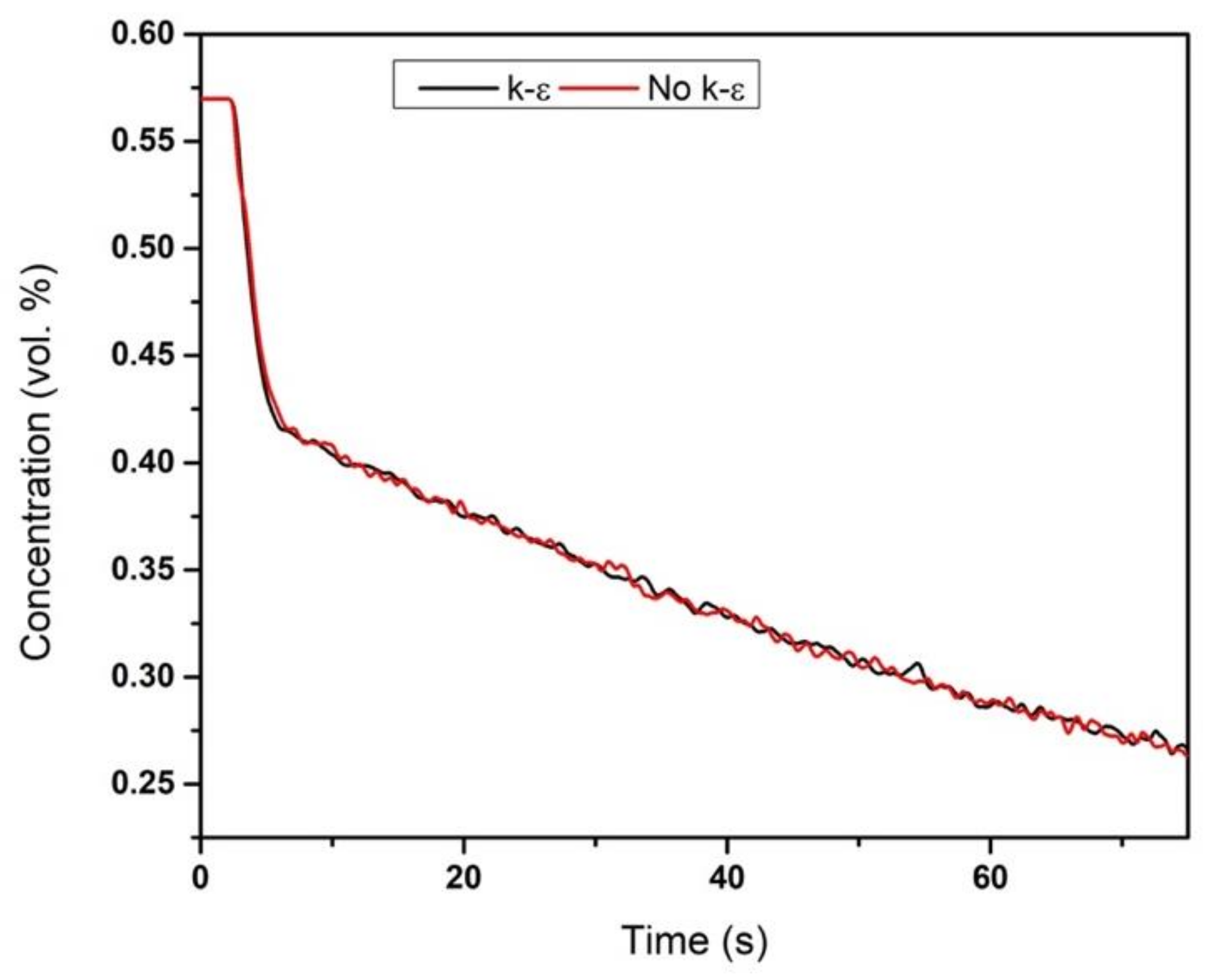
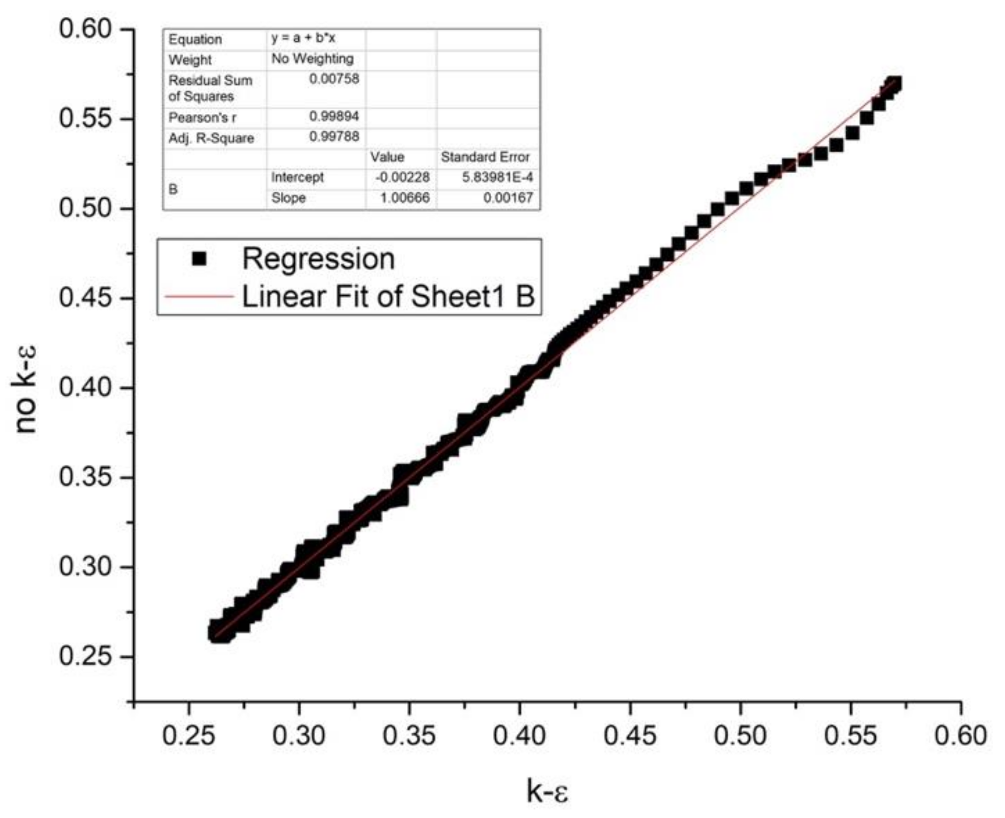
4.3. Sensitivity Analysis on the Approaches Used to Model Turbulence

After performing a sensitivity analysis on mesh refinement rate, also a sensitivity analysis on turbulence was performed. Results are shown in Figure 17 and Figure 18 and also in this case we see that the coefficient of correlation of the two data sets is higher than 0.99.

5. Conclusions

The Marie Curie IF project GTCLC-NEG wants to develop a carbon negative emissions technology for power generation, based on the coupling of a CLC combustor to a gas turbine. To do so both the air reactor and the fuel reactor have to be operated at pressurized conditions. To design and optimize the operation of a fuel reactor in pressurized conditions a CFD model has been developed in this work based on the MFIX 21.2 software (NETL US DOE, Houston, TX, USA). The model has been first tested at atomspheric conditions and results have been compared with available 0D models and main experimental campaigns performed in batch CLC reactors. The trends of the reaction products during time are correspondent to the results available in the literature. The only aspect to be optimized on the chemical reactions scheme (which is implemented in a User Defined Function) to account for the production of carbon monoxide, which has been detected in significant concentrations in the experimental campaigns. Another improvement will be that of the introduction of the distributor plate which is actually used in the plants of the Instituto de Carboquimica to insert the gas in the fuel reactor. Then the model will be tested at different pressures carefully adapting the kinetics of the reactions.

References

1. Cozzi, L.; Gould, T.; Bouckart, S.; Crow, D.; Kim, T.Y.; Mcglade, C. World Energy Outlook 2020; International Energy Agency: Paris, France, 2020; pp. 1–461. [Google Scholar] [CrossRef]
2. Chankov, G.; Hinov, N. The energy strategy and energy policy of the european union. Econ. Stud. 2021, 30, 3–31. [Google Scholar]
3. Yamagata, Y.; Hanasaki, N.; Ito, A.; Kinoshita, T.; Murakami, D.; Zhou, Q. Estimating water–food–ecosystem trade-offs for the global negative emission scenario (IPCC-RCP2. 6). Sustain. Sci. 2018, 13, 301–313. [Google Scholar] [CrossRef]
4. Osman, M. A Pressurized Internally Circulating Reactor (ICR) for Streamlining Development of Chemical Looping Technology. Ph.D. Thesis, Norwegian University of Science and Technology, Trondheim, Norway, 2021. [Google Scholar]
5. Abad, A.; Adánez, J.; García-Labiano, F.; De Diego, L.F.; Gayán, P. Modeling of the chemical-looping combustion of methane using a Cu-based oxygen-carrier. Combust. Flame 2010, 157, 602–615. [Google Scholar] [CrossRef] [Green Version]
6. Fulchini, F.; Ghadiri, M.; Borissova, A.; Amblard, B.; Bertholin, S.; Cloupet, A.; Yazdanpanah, M. Development of a methodology for predicting particle attrition in a cyclone by CFD-DEM. Powder Technol. 2019, 357, 21–32. [Google Scholar] [CrossRef]
7. Li, Z.; Xu, H.; Yang, W. Synergistic effect between CO2 and H2O on biomass chemical looping gasification with hematite as oxygen carrier. In Proceedings of the International Conference on Applied Energy 2019, Västerås, Sweden, 12–15 August 2019; Elsevier: Amsterdam, The Netherlands, 2019. [Google Scholar]
8. Chen, X.; Ma, J.; Tian, X.; Wan, J.; Zhao, H. CPFD simulation and optimization of a 50 kWth dual circulating fluidized bed reactor for chemical looping combustion of coal. Int. J. Greenh. Gas Control 2019, 90, 102800. [Google Scholar] [CrossRef]
9. Zhou, W.; Zhao, C.; Duan, L.; Qu, C.; Chen, X. Two-dimensional computational fluid dynamics simulation of coal combustion in a circulating fluidized bed combustor. Chem. Eng. J. 2011, 166, 306–314. [Google Scholar] [CrossRef]
10. Tabib, M.V.; Johansen, S.T.; Amini, S. A 3D CFD-DEM Methodology for Simulating Industrial Scale Packed Bed Chemical Looping Combustion Reactors. Ind. Eng. Chem. Res. 2013, 52, 12041–12058. [Google Scholar] [CrossRef]
11. Banerjee, S.; Agarwal, R. Transient reacting flow simulation of spouted fluidized bed for coal-direct chemical looping combustion with different Fe-based oxygen carriers. Appl. Energy 2015, 160, 552–560. [Google Scholar] [CrossRef]
12. Harichandan, A.B.; Shamim, T. CFD analysis of bubble hydrodynamics in a fuel reactor for a hydrogen-fueled chemical looping combustion system. Energy Convers. Manag. 2014, 86, 1010–1022. [Google Scholar] [CrossRef]
13. Alobaid, F.; Ohlemüller, P.; Ströhle, J.; Epple, B. Extended Euler–Euler model for the simulation of a 1 MWth chemical–looping pilot plant. Energy 2015, 93, 2395–2405. [Google Scholar] [CrossRef]
14. Kruggel-Emden, H.; Rickelt, S.; Stepanek, F.; Munjiza, A. Development and testing of an interconnected multiphase CFD-model for chemical looping combustion. Chem. Eng. Sci. 2010, 65, 4732–4745. [Google Scholar] [CrossRef]
15. Breault, R.W.; Weber, J.; Straub, D.; Bayham, S. Computational Fluid Dynamics Modeling of the Fuel Reactor in NETL’s 50 kWth Chemical Looping Facility. J. Energy Resour. Technol. 2017, 139, 042211. [Google Scholar] [CrossRef]
16. Li, S.; Shen, Y. Numerical study of gas-solid flow behaviors in the air reactor of coal-direct chemical looping combustion with Geldart D particles. Powder Technol. 2020, 361, 74–86. [Google Scholar] [CrossRef]
17. Porrazzo, R.; White, G.; Ocone, R. Fuel reactor modelling for chemical looping combustion: From micro-scale to macro-scale. Fuel 2016, 175, 87–98. [Google Scholar] [CrossRef] [Green Version]
18. Parker, J.M. CFD model for the simulation of chemical looping combustion. Powder Technol. 2014, 265, 47–53. [Google Scholar] [CrossRef]
19. Menon, K.G.; Patnaikuni, V.S. CFD simulation of fuel reactor for chemical looping combustion of Indian coal. Fuel 2017, 203, 90–101. [Google Scholar] [CrossRef]
20. Chen, L.; Yang, X.; Li, G.; Li, X.; Snape, C. Prediction of bubble fluidisation during chemical looping combustion using CFD simulation. Comput. Chem. Eng. 2017, 99, 82–95. [Google Scholar] [CrossRef]
21. Peng, Z.; Doroodchi, E.; Alghamdi, Y.A.; Shah, K.; Luo, C.; Moghtaderi, B. CFD–DEM simulation of solid circulation rate in the cold flow model of chemical looping systems. Chem. Eng. Res. Des. 2015, 95, 262–280. [Google Scholar] [CrossRef]
22. Shuai, W.; Yunchao, Y.; Huilin, L.; Jiaxing, W.; Pengfei, X.; Guodong, L. Hydrodynamic simulation of fuel-reactor in chemical looping combustion process. Chem. Eng. Res. Des. 2011, 89, 1501–1510. [Google Scholar] [CrossRef]
23. Lin, J.; Luo, K.; Sun, L.; Wang, S.; Hu, C.; Fan, J. Numerical Investigation of a Syngas-Fueled Chemical Looping Combustion System. Energy Fuels 2020, 34, 12800–12809. [Google Scholar] [CrossRef]
24. Reinking, Z.; Whitty, K.J.; Lighty, J.S. A simulation-based parametric study of CLOU chemical looping reactor performance. Fuel Process. Technol. 2021, 215, 106755. [Google Scholar] [CrossRef]
25. Hamidouche, Z.; Masi, E.; Fede, P.; Simonin, O.; Mayer, K.; Penthor, S. Unsteady three-dimensional theoretical model and numerical simulation of a 120-kW chemical looping combustion pilot plant. Chem. Eng. Sci. 2019, 193, 102–119. [Google Scholar] [CrossRef] [Green Version]
26. Ahmed, I.; De Lasa, H. CO2 Capture Using Chemical Looping Combustion from a Biomass-Derived Syngas Feedstock: Simulation of a Riser–Downer Scaled-Up Unit. Ind. Eng. Chem. Res. 2020, 59, 6900–6913. [Google Scholar] [CrossRef]
27. Seo, M.W.; Nguyen, T.D.; Lim, Y.I.; Kim, S.D.; Park, S.; Song, B.H.; Kim, Y.J. Solid circulation and loop-seal characteristics of a dual circulating fluidized bed: Experiments and CFD simulation. Chem. Eng. J. 2011, 168, 803–811. [Google Scholar] [CrossRef]
28. Van der Watt, J.G.; Laudal, D.; Krishnamoorthy, G.; Feilen, H.; Mann, M.; Shallbetter, R.; Nelson, T.; Srinivasachar, S. Development of a Spouted Bed Reactor for Chemical Looping Combustion. J. Energy Resour. Technol. 2018, 140, 112002. [Google Scholar] [CrossRef]
29. NETL. MFIX Open Source Multiphase Flow Modeling for Real-World Applications; National Energy Technology Laboratory: Pittsburgh, PA, USA, 2016.
30. Alobaid, F.; Almohammed, N.; Farid, M.M.; May, J.; Rößger, P.; Richter, A.; Epple, B. Progress in CFD Simulations of Fluidized Beds for Chemical and Energy Process Engineering. Prog. Energy Combust. Sci. 2021, 100930. [Google Scholar] [CrossRef]
31. Son, S.R.; Kim, S.D. Chemical-Looping Combustion with NiO and Fe2O3 in a Thermobalance and Circulating Fluidized Bed Reactor with Double Loops. Ind. Eng. Chem. Res. 2006, 45, 2689–2696. [Google Scholar] [CrossRef]
32. Abad, A.; Adanez, J.; García-Labiano, F.; De Diego, L.F.; Gayan, P.; Celaya, J. Mapping of the range of operational conditions for Cu-, Fe-, and Ni-based oxygen carriers in chemical-looping combustion. Chem. Eng. Sci. 2007, 62, 533–549. [Google Scholar] [CrossRef] [Green Version]
33. Adánez, J.; Gayán, P.; Celaya, J.; De Diego, L.F.; García-Labiano, F.; Abad, A. Chemical Looping Combustion in a 10 kWth Prototype Using a CuO/Al2O3 Oxygen Carrier: Effect of Operating Conditions on Methane Combustion. Ind. Eng. Chem. Res. 2006, 45, 6075–6080. [Google Scholar] [CrossRef]
34. Luis, F.; Garci, F.; Gayán, P.; Celaya, J.; Palacios, J.M.; Adánez, J. Operation of a 10 kWth chemical-looping combustor during 200 h with a CuO–Al2O3 oxygen carrier. Fuel 2007, 86, 1036–1045. [Google Scholar]
35. García-Labiano, F.; De Diego, L.F.; Adánez, J.; Abad, A.A.; Gayán, P. Reduction and Oxidation Kinetics of a Copper-Based Oxygen Carrier Prepared by Impregnation for Chemical-Looping Combustion. Ind. Eng. Chem. Res. 2004, 43, 8168–8177. [Google Scholar] [CrossRef]
36. Zerobin, F.; Penthor, S.; Bertsch, O.; Pröll, T. Fluidized bed reactor design study for pressurized chemical looping combustion of natural gas. Powder Technol. 2017, 316, 569–577. [Google Scholar] [CrossRef]
37. Wolf, J.; Anheden, M.; Yan, J. Comparison of nickel- and iron-based oxygen carriers in chemical looping combustion for CO2 capture in power generation. Fuel 2005, 84, 993–1006. [Google Scholar] [CrossRef]
38. Consonni, S.; Lozza, G.; Pelliccia, G.; Rossini, S.; Saviano, F. Chemical-Looping Combustion for Combined Cycles with CO2 Capture. J. Eng. Gas Turbines Power 2006, 128, 525–534. [Google Scholar] [CrossRef]
39. Li, T.; Dietiker, J.-F.; Shahnam, M. MFIX simulation of NETL/PSRI challenge problem of circulating fluidized bed. Chem. Eng. Sci. 2012, 84, 746–760. [Google Scholar] [CrossRef]
40. Gidaspow, D. Multiphase Flow and Fluidization: Continuum and Kinetic Theory Descriptions; Academic Press: Cambridge, MA, USA, 1994. [Google Scholar]
41. Lun, C.K.K.; Savage, S.B.; Jeffrey, D.J.; Chepurniy, N. Kinetic theories for granular flow: Inelastic particles in Couette flow and slightly inelastic particles in a general flowfield. J. Fluid Mech. 1984, 140, 223–256. [Google Scholar] [CrossRef]
42. Wen, C.Y. Mechanics of fluidization. Chem. Eng. Prog. Symp. Ser. 1966, 62, 100–111. [Google Scholar]
43. Ergun, S. Fluid flow through packed columns. Chem. Eng. Prog. 1952, 48, 89–94. [Google Scholar]
44. Benyahia, S.; Syamlal, M.; O’brien, T. Summary of MFIX Equations 2012. Available online: https://mfix.netl.doe.gov/doc/mfix-archive/mfix_current_documentation/MFIXEquations2012-1.pdf (accessed on 29 December 2021).
45. Syamlal, M. MFIX documentation numerical technique. MFIX Doc. Numer. Tech. 1998, 5824, 80. [Google Scholar] [CrossRef] [Green Version]
46. Syamlal, M.; Rogers, W.; O’brien, T.J. MFIX documentation theory guide. MFIX Doc. Theory Guide 1993. [Google Scholar] [CrossRef] [Green Version]
47. Cabello, A.; Abad, A.; García-Labiano, F.; Gayán, P.; De Diego, L.F.; Adánez, J. Kinetic determination of a highly reactive impregnated Fe2O3/Al2O3 oxygen carrier for use in gas-fueled chemical looping combustion. Chem. Eng. J. 2014, 258, 265–280. [Google Scholar] [CrossRef] [Green Version]
48. Mora, J.C.; Nederstigt, Y.C.M.; Hill, J.M.; Ponnurangam, S. Promoting Effect of Supports with Oxygen Vacancies as Extrinsic Defects on the Reduction of Iron Oxide. J. Phys. Chem. C 2021, 125, 14299–14310. [Google Scholar] [CrossRef]
49. Abad, A.; Adánez, J.; Cuadrat, A.; García-Labiano, F.; Gayán, P.; De Diego, L.F. Kinetics of redox reactions of ilmenite for chemical-looping combustion. Chem. Eng. Sci. 2011, 66, 689–702. [Google Scholar] [CrossRef] [Green Version]
50. Abanades, J.C.; Abdel-Ghani, M.; Abdelkarim, A.; Abe, E.; Abe, Y.; Abouzeid, A.Z. Cumulative Author Index of Volumes 50–75. Powder Technol. 1993, 75, 209–216. [Google Scholar]
51. Leonard, B.P.; Mokhtari, S. Beyond first-order upwinding: The ultra-sharp alternative for non-oscillatory steady-state simulation of convection. Int. J. Numer. Methods Eng. 1990, 30, 729–766. [Google Scholar] [CrossRef]
52. Patankar, S.V. Numerical Heat Transfer and Fluid Flow; Hemisphere Publishing: New York, NY, USA, 1980; ISBN 9781315275130. [Google Scholar]
53. Spalding, D.B. Numerical computation of multi-phase fluid flow and heat transfer. In Von Karman Institute for Fluid Dynamics Numerical Computation of Multi-Phase Flows; Imperial College: London, UK, 1981; pp. 161–191. [Google Scholar]
54. Harlow, F.H.; Amsden, A.A. Numerical calculation of multiphase fluid flow. J. Comput. Phys. 1975, 17, 19–52. [Google Scholar] [CrossRef]
55. Rivard, W.; Torrey, M. K-FIX: A Computer Program for Transient, Two-Dimensional, Two-Fluid Flow; Los Alamos Scientific Lab: Los Alamos, NM, USA, 1976. [Google Scholar]
56. Kotteda, V.M.K.; Kumar, V.; Spotz, W. Performance of preconditioned iterative solvers in MFiX–Trilinos for fluidized beds. J. Supercomput. 2018, 74, 4104–4126. [Google Scholar] [CrossRef]
57. Van der Vorst, H.A. Bi-CGSTAB: A fast and smoothly converging variant of Bi-CG for the solution of nonsymmetric linear systems. SIAM J. Sci. Stat. Comput. 1992, 13, 631–644. [Google Scholar] [CrossRef]
58. Abad, A.; Adanez, J.; De Diego, L.F.; Gayan, P.; García-Labiano, F.; Lyngfelt, A. Fuel reactor model validation: Assessment of the key parameters affecting the chemical-looping combustion of coal. Int. J. Greenh. Gas Control 2013, 19, 541–551. [Google Scholar] [CrossRef] [Green Version]
59. Abad, A.; Gayán, P.; De Diego, L.F.; García-Labiano, F.; Adánez, J. Fuel reactor modelling in chemical-looping combustion of coal: 1. Model formulation. Chem. Eng. Sci. 2013, 87, 277–293. [Google Scholar] [CrossRef] [Green Version]
60. Abad, A.; Mattisson, T.; Lyngfelt, A.; Johansson, M. The use of iron oxide as oxygen carrier in a chemical-looping reactor. Fuel 2007, 86, 1021–1035. [Google Scholar] [CrossRef]
61. Peng, Z.; Doroodchi, E.; Alghamdi, Y.; Moghtaderi, B. Mixing and segregation of solid mixtures in bubbling fluidized beds under conditions pertinent to the fuel reactor of a chemical looping system. Powder Technol. 2013, 235, 823–837. [Google Scholar] [CrossRef]
62. Pans, M.A.; Gayán, P.; Abad, A.; García-Labiano, F.; De Diego, L.F.; Adánez, J. Use of chemically and physically mixed iron and nickel oxides as oxygen carriers for gas combustion in a CLC process. Fuel Process. Technol. 2013, 115, 152–163. [Google Scholar] [CrossRef] [Green Version]
Figure 1. GTCLC-NEG plant layout.
Processes 10 00588 g001
Figure 2. Fluidized bed reactor geometry.
Processes 10 00588 g002
Figure 3. The oxygen carrier (Fe2O3(Al2O3)).
Processes 10 00588 g003
Figure 4. Final mesh (14,000 cells)—left, cells distribution in the bed—right.
Processes 10 00588 g004
Figure 5. Modeling platform.
Processes 10 00588 g005
Figure 6. Gas Velocity Magnitude at a section located in the middle of the reactor.
Processes 10 00588 g006
Figure 7. Average temperature inside the reactor; the line corresponds to the average value, which is derived through statistical calculations which also calculate the quartiles of the temperature distribution at a given time (that are indicated in a stronger color and are closer to the average) and the extreme values which are the lower and upper limit of the temperature distribution (that are indicated in a more light color and are more external respect to the quartiles).
Processes 10 00588 g007
Figure 8. Average gas velocity in the reactor; the line corresponds to the average value, which is derived through statistical calculation which also calculate the quartiles of the velocity distribution at a given time (that are indicated in a stronger color and are closer to the average) and the extreme values which are the lower and upper limit of the velocity distribution (that are indicated in a more light color and are more external respect to the quartiles).
Processes 10 00588 g008
Figure 9. Average volumetric flow inside the reactor; the line corresponds to the average value, which is derived through statistical calculation which also calculate the quartiles of the volumetric flow distribution at a given time (that are indicated in a more stronger color and are more close to the average) and the extreme values which are the lower and upper limit of the volumetric flow distribution (that are indicated in a more light color and are more external respect to the quartiles).
Processes 10 00588 g009
Figure 10. Contours of biomethane mass fraction in the reactor, at different times.
Processes 10 00588 g010
Figure 11. Gas concentrations at the outlet, during time (normalized on the mixture obtained by previously subtracting nitrogen). Processes 10 00588 i001 is taken from [60] Processes 10 00588 i002 is taken from [60] Processes 10 00588 i003 is taken from [60].
Processes 10 00588 g011
Figure 12. Bed height increase.
Processes 10 00588 g012
Figure 13. Concentration of Fe2O3 in the bed at different times.
Processes 10 00588 g013
Figure 14. Conversion of the oxygen carriers (left); Reaction rates during time (right). The line corresponds to the average value, which is derived through statistical calculation which also calculate the quartiles of the volumetric flow distribution at a given time (that are indicated in a stronger color and are more close to the average) and the extreme values which are the lower and upper limit of the volumetric flow distribution (that are indicated in a more light color and are more external respect to the quartiles).
Processes 10 00588 g014
Figure 15. Comparison between the mass fraction of biomethane during time obtained with the refined mesh (mesh>) and the one obtained with the loose mesh (mesh<).
Processes 10 00588 g015
Figure 16. Regression analysis performed on the data on the mass fraction of biomethane during time obtained with the refined mesh (mesh>) and the one obtained with the loose mesh (mesh<).
Processes 10 00588 g016
Figure 17. Comparison between the biomethane mass fraction obtained with and without k-epsilon to describe turbulence.
Processes 10 00588 g017
Figure 18. Regression analysis performed on the data two simulations: one using k-epsilon model and the other not using it.
Processes 10 00588 g018