
Research on Fault Diagnosis of PST Electro-Hydraulic Control System of Heavy Tractor Based on Support Vector Machine


Department of Traffic and Vehicle Engineering, Shandong University of Technology, Zibo 255000, China
*
Author to whom correspondence should be addressed.
Processes 2022, 10(4), 791; https://doi.org/10.3390/pr10040791
Submission received: 14 March 2022
/
Revised: 12 April 2022
/
Accepted: 14 April 2022
/
Published: 18 April 2022
(This article belongs to the Special Issue Application of Fuzzy Control in Computational Intelligence)
Abstract
:Due to the harsh working environment of the tractor, the transmission can often be faulty. In order to ensure the reliability of its operation, it must be monitored and the fault discovered. In this paper, the support vector machine (SVM) method is used. The eigenvector conversion of the original data uses the following eigenvectors: Three fault modes (leakage fault of shift clutch hydraulic cylinder, blockage fault of oil passage, and blockage fault of proportional valve spool) are identified in matrix and laboratory (MATLAB) with the help of the library for support vector machines (LibSVM) toolkit, and the classification accuracy of test samples is 90%. The normal mode of the PST electro-hydraulic system and the three kinds of fault modes mentioned above are discriminated against, and the correct rate of fault diagnosis reaches 95%, which meets the needs of practical engineering. Analysis of the fault recording data of the power shifting transmission shift solenoid valve shows that the difference between fault pressure data and normal data is small, and the value of traffic data is greater. This method can realize the fault mode online recognition based on controller area network (CAN) communication, and the research results provide a theoretical basis for the fault diagnosis of the PST electro-hydraulic control system.
1. Introduction
At present, more and more electronic equipment and electronic control technology is being used in agricultural tractors, which greatly improves the working performance of tractors. However, frequent gear shifts in the process of operation easily lead to faults in the tractor’s electro-hydraulic system, the faults of the electro-hydraulic system have strong coupling, and different faults have similar manifestations. Therefore, it is difficult to determine the fault points of an electro-hydraulic system, which increases the difficulty of fault diagnosis. According to the flow and pressure signals of the shift solenoid valve collected by the tractor power-shift transmission (PST) node system, some fault diagnosis methods are adopted to complete online fault diagnosis and improve the working efficiency of the tractor controller area network (CAN) communication network; the Transmission Control Unit (TCU) is an important node in the CAN communication network. At present, many scholars have studied the fault diagnosis of tractor power shifting transmissions. In 2009, Kaveh Mollazade and others used vibration signals and power spectral density frequencies to determine the hydraulic pump’s failure [1]. In 2013, Ebrahim and colleagues obtained the fault vibration signal of the MP285 tractor gearbox, converted the signal to the frequency domain, selected important features using a genetic algorithm, and then trained the input and output using a neural network, with the accuracy of fault diagnosis and classification reaching 99.9% [2]. In 2017, the accuracy of fault diagnosis and classification reached 99.9%. Chunyin Wu and others developed the tractor fault diagnosis expert system, using the fault tree analysis method and supporting two-way reasoning, forwarding the reason and reverse reasoning interpretation algorithm, providing an understanding of the derivation structure [3]. In 2002, Chi Yuan collected a large amount of agricultural hydraulic system fault information and established a fault diagnosis knowledge base by applying Visual Basic (VB) 6.0, the fault diagnosis expert system of agricultural machinery hydraulic systems, using the fault tree diagnosis model, depth priority search and forward-reasoning strategies, as well as implementing fault diagnosis and eliminating the purpose of troubleshooting [4]. Jiangsu University’s Li Boquan team investigated tractor gearbox gear fault diagnosis in 2003, employing wavelet analysis and a genetic algorithm to recognize fault patterns [5,6]. In 2008, Zhang Xinhai used data driver forwarding strategies with a three-layer back propagation (BP) neural network tool for mechanical fault diagnosis [7]. This method needs further research. In 2011, Zhao Shuang achieved fault diagnosis of gearbox gears using a support vector machine multi-class classifier [8]. In 2015, Wang Guangming reported that he could diagnose hydraulic faults in hydraulic-sleeved transmissions based on the Fisher criteria and nuclear method, process the acquired fault data, and then learn and train using rough sets and characteristics of the quantity method for rough samples, streamlining test samples so they can be classified correctly [9]. Through the above document, there is still less research on the tractor power shift transmission. The fault diagnosis method is mainly the expert system, and a large amount of fault data is required to support it. In fact, the power shift transmission fault data is difficult to collect; the amount of fault data is small, it is difficult to diagnose the fault with a realistic diagnosis, and the fault point is difficult to determine.
In this paper, a tractor with full power shift transmission developed independently is seen as the research object. At present, there is little research on the diagnosis of faults in the electro-hydraulic system of power shift transmission, so it is necessary to consider and explore this field. The application layer of the CAN bus contains the data frame of the shift solenoid valve parameters. The fault diagnosis: The Electronic Control Unit (ECU) obtains real data through CAN network data sharing, monitors the status of transmission, and diagnoses the faults of electro-hydraulic systems through data analysis and operation, as well as analyzing the characteristics of each fault by simulating the flow or clutch pressure response of the proportional valve in fault mode, screening and processing previous fault record data, utilizing the support vector machine (SVM) classification method, and utilizing the library for support vector machines (LibSVM) toolkit to realize real-time fault pattern recognition in matrix and laboratory (MATLAB).
2. Failure Analysis of PST Electro-Hydraulic System
2.1. How a Full Power Shift Transmission Works
PST is an important transmission device, which is mainly used for heavy-duty vehicles and hydraulically driven wheeled construction machinery or agricultural machinery. Its basic structure is a hydraulic-mechanical system without a main clutch. The shift actuator is a hydraulically driven multi-plate wet clutch. The shift operation can be achieved through the shift solenoid valve. The power transmission is marked by no interruption of power, fast shift speed, and no impact. In this paper, a fixed-shaft multi-shaft tandem structure power shift transmission is designed, including power shift and power shift parts; all gears can realize the power shift, so it is called a “full power shift transmission.” Figure 1 shows the internal structure of the full power shift transmission designed in this paper, which consists of a main transmission device and an auxiliary transmission device, which are connected in parallel.
Electro-Hydraulic Proportional Control System
Figure 2 shows the electro-hydraulic control system of the PST. The single-chip microcomputer is the control part, and the hydraulic module is the execution part. The hydraulic module is split into a pressure regulation module and a cooling and lubrication module (L1, L2, L3).
In the power shift transmission designed in this paper, the most critical is the shift proportional solenoid valve. The structure of the shift proportional solenoid valve is shown in Figure 3. The shift proportional solenoid valve is composed of an adjusting screw, an adjusting spring, a valve sleeve, a coil, an armature, a valve body, a valve baffle, a valve core, and an oil inlet ball valve. It works on the principle that the position of the adjustment screw determines the preset pressure. The coil is energized to generate a magnetic field, attracting the armature to the approach. The ball valve moves to the left, and pressure oil fills the clutch oil circuit. The magnitude of the current determines the strength of the magnetic field and the degree to which the oil inlet is opened. By adjusting the duty ratio of the Pulse Width Modulation (PWM) signal to control the size of the opening current, the continuous adjustment of the pressure and flow is realized, and the soft engagement of the shift clutch is controlled.
The valve port of the shift proportional solenoid valve is generally a cone valve or a ball valve structure, and an annular gap will be formed between the valve core and the valve seat during the opening and closing process, resulting in a throttling effect. The flow characteristics through this gap are:
In the formula, is the flow coefficient is the flow area of the valve port, m2; is the pressure difference between the inlet and outlet of the solenoid valve, , Pa; and are the inlet and outlet pressures of the proportional solenoid valve, respectively; and is the oil density, kg/m3.
The flow coefficient is usually related to the Reynolds coefficient flowing through the gap of the valve port, as well as the geometry and size of the valve port, etc. It is a very complex dimensionless coefficient. The flow coefficient under a certain condition is usually obtained by experiments, and the general value range is 0.60–0.80.
The oil pressure of the shift clutch cylinder can be expressed as:
In the formula, is the system oil pressure, about 2 MPa.
At present, the shift proportional solenoid valve of the pressure regulation module mostly adopts an open-loop control method without signal feedback. For example, the shift control signal of a power shift transmission of Lovol Apos is illustrated in Figure 4. The electrical signal range is 340–1100 mA. After being supplemented by the amplifier, it sends a DC current to the proportional electromagnet of the electro-hydraulic proportional valve. The proportional electromagnetic force is generated in proportion to pushing the spool to produce the corresponding displacement, thereby controlling the flow, pressure, and direction of the hydraulic oil entering the multi-plate wet clutch and the clutch friction plates from slipping to engaging, so that the load obtains the corresponding force, displacement, and speed. The accumulator can buffer pressure in the system and play the role of regulating flow and pressure.
2.2. Electronic Control System Failure
Electronic control system faults are divided into sensor faults, electronic control unit faults, electronic control element circuits, and CAN communication faults, as shown in Table 1.
TCU control of the power gear in the automatic mode. The more gears, the greater the control difficulty. The main input and output signals of the TCU are presented in Figure 5. The input signals of the PST control unit mainly include the driver’s driving intention signal, the engine speed torque signal, the shift actuator feedback signal, the final drive, and the walking system signal, etc. The PST- Electronic Control Unit (ECU) needs to calculate a reasonable shift control law according to a certain judgment logic or algorithm for the above signals and realize the control of the shift actuator—the shift solenoid valve.
The shifting process is illustrated in Figure 6. The electronic control network sends messages through the CAN bus. The communication module chooses to accept the relevant messages from the CAN bus and converts them into the data required for the controller to compute. After the data processing module processes and converts some of the signals, it is sent to the shift decision module, and the control current of the shift solenoid valve is formed after the calculation of multiple signals, which indirectly control the hydraulic oil pressure and complete a power shift.
Each signal is produced by its corresponding sensor. Once the sensor fails, it will influence the decision-making of the controller. Types of sensor faults can be divided into voltage-based faults and time-based faults. The probability of the intramural program’s runaway failure of the electronic control unit is small. Once it occurs, the TCU will no longer communicate with the VCU, and the VCU will respond according to a reliable fault tolerance strategy to ensure the safety of operation or driving. CAN communication failure is manifested as the failure of the VCU to receive the TCU signal and the loss of some TCU signals. When the pressure reducing valve or the gear solenoid valve fails, the gear selection and shifting disorder occurs. That is, the shifting clutch cannot execute the selection and shifting commands of the TCU. For the fault diagnosis of the shifting mechanism, the actual gear and the gear sensor displayed by the speed ratio of the input shaft and the output shaft are used to display the gear, and the TCU needs the gear to analyze the redundancy between the three so as to accurately diagnose the fault condition [10].
2.3. PST Hydraulic System Failure
Due to the sudden change of direction of the shift solenoid valve and the engagement or separation of the shift clutch, a pressure shock will be generated in the electro-hydraulic system, causing the system pressure to fluctuate rapidly in a short period of time, easily causing damage to the control elements and sealing devices and causing vibration and noise. Electro-hydraulic system failures include pump-motor system failure, proportional reversing valve failure, shift clutch failure, etc., as well as any component of the hydraulic system such as the charge pump, cooler, and pipeline related to it; common transmission failures and failure caused by the maintenance method are shown in Table 2.
The traditional fault diagnosis method is manual inspection, and the cause of the fault and the fault location are determined and repaired through the methods of mechanical inspection and hydraulic inspection. Among them, hydraulic detection looks for faults in three aspects: the oil level of the transmission oil pans, the oil leakage of the shifting clutch, and the cooling and lubricating oil amount of the torque converter. For example, if the oil level in the transmission oil pan is low, the clutch operating pressure will be low and the output flow of the torque converter charge pump will be insufficient. The oil level of the transmission oil pan is monitored by installing a liquid level sensor, and the liquid level data are displayed on the instrument. With an alarm when the oil level is low, such failure can be avoided. When the seal ring of the clutch cylinder or the seal connected to it is damaged, the system will have a large leakage. The leakage and the degree of damage can be judged by the data measured by the flow sensor of the clutch oil inlet pipeline. The flow simulation curve of the clutch leakage failure mode is shown in Figure 7a, and the area difference between the green dotted line and the red solid line represents the leakage amount. Under normal conditions, the leakage of all shift clutches is basically the same. If the leakage of one of the clutches exceeds the standard, the clutch should be checked and repaired immediately. Figure 7b shows the flow change curve of the clutch oil filling process in blocking mode. The response of the whole process lags, and the maximum value is always lower than the maximum value in the normal state. The more severe the lag and the smaller the flow, the more severe the blockage.
3. Fault Diagnosis of PST Electro-Liquid System Based on CAN Bus Network
3.1. Fault Diagnosis Principle
The traditional fault diagnosis method is manual inspection, which relies on skilled engineers and experts to deal with the problems that affect the efficiency of tractor operation. The fault diagnosis of the tractor PST electro-hydraulic system based on the CAN network relies on the analysis of various sensors, the fault diagnosis ECU, and the prompt and alarm of the instrument/virtual terminal to complete the fault diagnosis and obtain maintenance. Based on the CAN bus, the principle of fault diagnosis, as shown in Figure 8, the fault diagnosis process requires the equipment bus, the tractor bus, and multiple modules, and the information acquisition module collects the flow of each shift solenoid valve. Through the VCU gateway completion information in the network, the fault diagnosis of the ECU determines the fault point and the fault type, then displays the exact fault information through the meter/virtual terminal or alert to complete the task of troubleshooting. At present, commonly used intelligent algorithms are Fuzzy Logic Algorithms (FLA), Neural Network Algorithms (NNA), SVM, and so on. The FLA depends on the establishment of a knowledge base, the performance of the inference engine, and expert experience. The NNA needs a lot of sample data for its training network, and it is not difficult to fall into a local optimum. The test sample data for this experiment have the characteristics of a small sample size and high dimensionality. SVM has a good classification and generalization ability when there are very few samples and has superior ability in classification and prediction. For high-dimensional nonlinear problems, SVM can be transformed into linear problems by constructing linear discriminant functions in high-dimensional space, so the complexity of the SVM algorithm will not have anything to do with the dimension of vectors. Moreover, the algorithm will be transformed into a convex quadratic programming problem with linear constraints. In theory, the global optimal solution can still be found, and the local extremum problem in NNA and other methods can be addressed. In view of the limited number of samples obtained in this paper, it has been decided to adopt the support vector machine algorithm to identify several failure modes online and use the support vector machine as the core algorithm of the fault diagnosis module of ECU power shift fault diagnosis.
3.2. SVM Principle
SVM is a new learning method in statistical learning theory that adopts the principle of structural risk minimization [10]. It shows many advantages in pattern recognition or the classification of small samples, as well as nonlinear and high-dimensional data samples, and has a strong generalization ability, which can realize linear and nonlinear classification problems.
3.2.1. Linear Scalability
The basic idea of SVM can be explained using the example of two-dimensional data samples in Figure 9. Black spots and white spots are two different samples, and in the case of linearity, the sample is set to (xi, yi), i = 1,2,…, m, xi ∈ Rd, yi ∈ {+1,−1} and the linear discrimination function is f(x) = ωx + b, that is, the classification plane is:
![Processes 10 00791 g009]()
ωx + b = 0
Figure 9.
Optimal classification surface in two-dimensional.
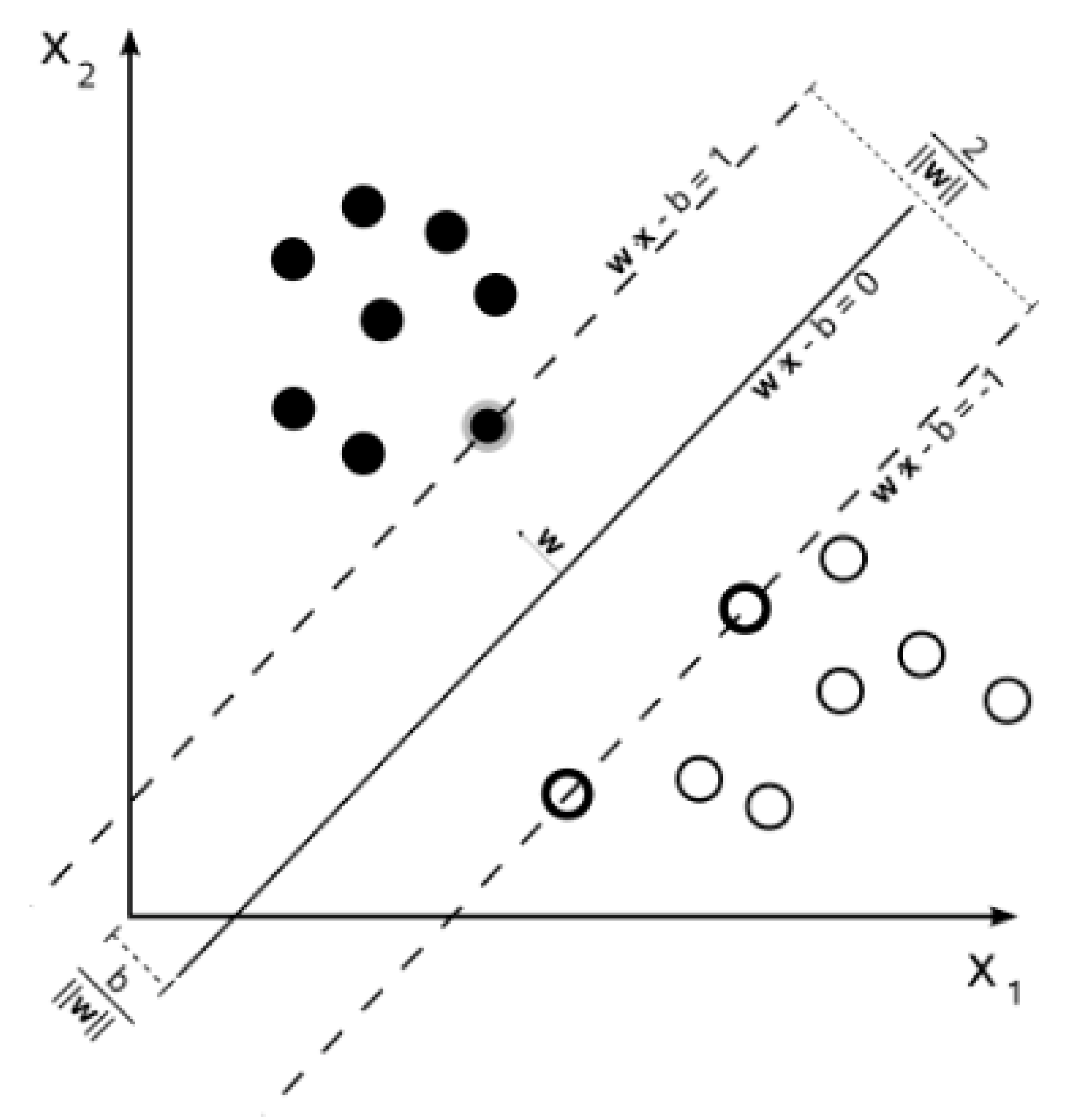
The two-dimensional extension of the multidimensional = (ω1, ω2, ωn) classified super plane’s space is as follows:
ωTx + b = 0
Two types of samples in multidimensional space can be expressed as:
There are also some data points distributed on the super plane ωTx + b = ±1, called the support vector, it is also a support vector to separate the data points in the multidimensional space.
According to the geometric relationship, the distance from the support vector to the optimal plane is , and the classification interval is . Make the classification interval to obtain the optimal plane. The constraints are located on both sides of the super plane to obtain an inequality constraint optimization problem:
For convenience of calculation, the transformation of the above formula into the minimization problem proceeds as follows:
Equation (7) is a convex quadratic programming problem. In order to further simplify the solution, it is transformed into a Lagrange dual problem, and the corresponding Lagrange multiplier αi > 0 is set for the inequality constraints of Equation (7). Obtain the Lagrange function ω, b of the original problem:
The optimization goal is: , for the Lagrange function to seek its minimum and questions about αi, just a deflection is zero, then connect Equation (8) to get ω, b, αi:
As seen from the Equation (9), by minimizing ω,b so that it is small, the optimization function is only the α parameter. This problem is to solve the sequential minimal optimization (SMO) algorithm [11], solving the α* value of α. If α* is the optimal solution, the above-described dual problem has a unique solution (ω*, b*), and it is:
In the Equation (10), the non-zero corresponding sample is a support vector, so the power coefficient vector of the optimal classification surface is a linear combination of support vectors, and b* is the classified threshold, so it can be solved by constraint conditions αi[yi(ωixi + b) − 1] = 0. Solving the above problems, the optimal classification surface function is:
3.2.2. Linear Indiscriminate Problem
At data acquisition, there is noise data, so that the original simple classification becomes linear. The SVM introduces the loan tolerance mechanism of the slack variable and the penalty factor, forming the algorithm itself, so that the distance from the classification plane does not narrow, and the soft interval is realized. In this classification, linear inseparable problems are described as:
In the Equation (12), ξ is a relaxation variable, indicating that the data point is far from the classification plane, and C is a penalty factor, which controls the degree of penalty of the missed data point. The Lagrange function is as follows:
In Equation (13), αi and βi are non-negative Lagrange multipliers, and an optimization problem can be converted to the occasional problem by seeking ω, b and ξ:
Several cases of solving αi are: ① αi = 0; ② 0 < αi < C; ③ αi = C. ②, ③ correspond to the support vector xi, where xi is called ② standard support vector, and xi in ③ is called a boundary support vector. If the solution to the optimization problem is α*= (α*1, α*2, L, αn) T:
By solving the above problems, ultimately transforming linearized inseparable problems into linear can be linear, and the optimal classification surface function can be obtained.
3.2.3. Low-Dimensional Space Nonlinear Problem
When the data set is inadequate in the low-dimensional space, the data set is mapped to the high-dimensional space through the core function. If the data set in the high dimension is linear, the super plane is expressed as:
ωTφ(x) + b = 0
Derived from the form of Equation (16)
φ(xi)Tφ(xj)T in Equation (17) is regarded as a whole, and a function of xi and xj, namely κ (xi, xj) = φ(xi)Tφ(xj)T; κ (xi, xj) is called the kernel function. Commonly used kernel functions include linear kernel functions, polynomial kernel functions, Gaussian kernel functions, and Sigmoid kernel functions.
In fact, the kernel function has no fixed form, and can be understood as a tool for mapping data sets from low-dimensional space to high-dimensional space. Figure 10 vividly shows the mapping function of the Gaussian kernel function. Experience shows that the Gaussian kernel function has the best mapping effect.
To sum up, the application of SVM in classification can be divided into two situations: (1) a linear classification problem; (2) a nonlinear classification problem. The problem (1) can be divided into two cases: ① When the problem is linearly separable, only the classified linear function (two-dimensional space) under the linear constraint condition is needed, and the structural risk is 0. ② When the problem is linearly indivisible, penalty factor C and relaxation variable ξ should be introduced, where ξ is the degree of “tolerance” to the wrong sample, C is the degree of punishment for this kind of “tolerance”, the soft interval realizes the sample separability, and the structural risk is not higher than C. In problem (2), the linear inseparability of low-dimensional space is mapped to high-dimensional space by the kernel function, thus realizing linear separability.
3.2.4. Solution of SVM in Multi-Class Classification Problem
At present, the multi-class promotion of SVM mainly adopts two methods: multi-objective optimization and combination coding [12]. The multi-objective optimization method solves all classification problems at once, and combination coding is realized by constructing multiple two-class SVMs with the following specific methods [13], as shown in Table 3.
4. An Example of Fault Classification Prediction and Result Analysis
4.1. Fault Case Analysis
According to the data recorded in the past, the faults of the hydraulic subsystem of the shift clutch mainly include leakage faults caused by poor sealing, oil passage blockage faults, and valve core jam faults.
4.1.1. Normal Mode
When the shift clutch works normally, the oil pressure, flow rate and other indicators are normal, the shift clutch moves quickly, the combination is smooth, there is no power interruption and impact in the shift process, and the pressure is constant.
4.1.2. Sealing Ring Damage and Leakage Fault
With frequent use or improper operation, the sealing ring inside the wet shift clutch is easily affected by friction heat, which causes deformation and damage, resulting in clutch oil leakage fault.
4.1.3. Oil Passage Blockage Fault
The hydraulic system has to be polluted by dust and other solid particles in the air, so the phenomenon of oil passage blockage is very common. In the electro-hydraulic system for proportional control of the shifting clutch studied in this paper, the outlet joint between the solenoid valve plate and the valve core is most prone to blockage. The accumulation of impurities reduces the diameter of the pipeline, decreases the flow rate in and out of the clutch cylinder, and increases the time of oil charging and discharging. The increase in oil charging and discharging will lead to more friction heat when the shift clutch goes hand in hand with power, which will aggravate the wear and even burn off the clutch.
4.1.4. Proportional Valve Spool Jam Fault
When the return spring of the proportional valve fails, it cannot return normally, and the oil cylinder of the shift clutch keeps the engagement pressure all the time, which leads to a large number of sliding wear losses caused by the friction plate being in a sliding wear state for a long time, and the generated heat will cause the friction plate to burn down, which is a very serious fault.
By analyzing the fault record data of the shift solenoid valve of power shift transmission, it is found that the difference between fault pressure data and normal data is small, and the increment of flow data fluctuates greatly. The following eigenvectors are used to transform the original data: root mean square value XRMS, peak factor C, kurtosis factor K, pulse factor I, and waveform factor S [14], which are defined as follows:
Report to the general assembly on the flow rate. The difference between the pressure data and the normal data is poor. For the convenience of calculation and processing, only the root means square value XRMS-P is considered. The flow rate and pressure value of the first second after the change section are taken, and the sampling point interval of the data is 0.05 s. T, F1, F2, and F3 are used to represent normal mode, hydraulic cylinder leakage of the shift clutch, oil passage blockage, and valve core blockage of the proportional valve, respectively. Table 4 indicates the sample data of the eigenvector after fault data processing.
4.2. Application of LibSVM in MATLAB
LibSVM software is a simple, fast, and effective software for SVM pattern recognition and regression. The software can solve classification problems such as C-SVC and v-SVC, one-class SVM distribution estimation problems, epsilon-SVR, and v-SVR regression problems. Four kernel function types are provided: linear kernel, polynomial kernel, radial basis function, and sigmoid kernel. In addition, the kernel function dimension d, the slack variable parameter γ of the kernel function, the penalty factor e, and other parameters is set, and the selected type only needs to be indicated when writing the program. LibSVM software can effectively solve multi-class classification problems, select parameters for cross-validation, weight unbalanced samples, and estimate the probability of multi-class problems [15]. In this paper, the software of this version is selected to be installed in Matlab2013a to realize the construction of a computer analysis environment.
The number of training samples selected in this paper is 5. That is, training and predictive sample sets of each pattern are 5. This paper uses the default C-SVC classifier to classify and diagnose, and implements the following steps:
- Select “Matlab2013a\toolbox\libsvm3.23\windows” path in Matlab’s control window, establish a dataset “mat” file “truedatas.mat, faultdatas1.mat, faultdatas2.mat, faultdatas3.mat” and a category label set “lableset1.mat, lableset2.mat, lableset3.mat, lableset4.mat”.
- Making the training set and test set data, the call function mapminmax scaled the test set to the [0,1] section.
- Test Set Sample Training Requires calls Svmtrain function, model = svmtrain(training_label_vector, training_instance_matrix,’libsvm_options’);where libsvm_options options include SVM type, core function type, core function parameter selection. In this document model = svmtrain(train_set_labels, train_set, ‘-c 1 -g 0.07’);’-c 1 -g 0.07’ omitted the SVM type, the default is C-SVC, omitted the core function type, the default is the radial base RBF, the default value of the parameter C is 1, g default value 1/k (k is sample data) Dimension, this article k = 6), the fault tolerant factor is 0.07.
- Using the grid search method to find the optimal C and g combination, select the value setting for gamma in [0.001,0.01,0.1,1,10,100]: for C in [0.001,0.01,0.1,1,10,100]:, then call the command svm = SVC(gamma = gamma, C=C), conduct a training for each combination, and then find a large set of parameter values for the minimum error to find the value of g = 0.001, C = 100. This method is time consuming, but it can accurately find the best parameters. The prediction set is classified by the model described above, and the Svmpredict function, [predict_label] = svmpredict (test_set_labels, test_set, model); the predictive sample test_set is corresponding to the label set test_set_labels, and the classification correct rate can be calculated.
4.3. Test Results Analysis
The outputs of T, F1, F2 and F3 are represented by numbers 0, 1, 2 and 3, respectively. The classification results of the prediction set in the sample set in Table 1 are shown in Figure 11, which shows the classification results more intuitively. The results show that two samples of F1 failure mode are incorrectly predicted as normal mode, but all the samples of other failure modes are correctly predicted. Therefore, the classification accuracy of predicted samples is 90%.
optimization finished, #iter = 5
nu = 1.000000
obj = −7.183243, rho = −0.025135
nSV = 10, nBSV = 10
Total nSV = 20
Accuracy = 90% (18/20) (classification)
A Fisher criterion is introduced here to analyze the diagnosis error of F1 internal leakage fault, and its principle will not be described in detail [16]. If the intra-class dispersion value of a feature is smaller and the inter-class dispersion value is larger, the Fisher criterion value is higher. According to pairwise discrimination, the Fisher criterion for calculating the characteristic variables of F1-F3 and T modes is shown in Table 5:
F2 has a larger Fisher criterion value of 3.253002, and F3 has a larger Fisher criterion value of 1.369812 and 6.105690, so the accuracy rate is higher when predicting classification, and each Fisher criterion value of F1 is very small. The reason is that the occurrence of faults has a gradual change, which is difficult to detect in the initial stage of internal leakage. Only when the damage degree of shift clutch piston changes from quantitative change to qualitative change will the system be strongly affected.
Due to the limited samples of the prediction set, this paper will use all 40 samples to further test the model, and the simulation results are shown in Figure 12.
optimization finished, #iter = 5
obj = −7.647503, rho = −0.015225
nSV = 10, nBSV = 10
Total nSV = 20
Accuracy = 95% (38/40) (classification)
From the running results, misclassified samples are still two samples of F1 failure mode, and all other samples are correctly identified. The increase of the number of test samples further improves the prediction accuracy to 95%.
4.4. Factors Affecting the Correctness of Classification
4.4.1. Training Sample Quantity
The literature was verified by simulation and concluded that the accuracy of leakage diagnosis of hydraulic systems would not increase with the increase of training samples, indicating that SVM has a significant advantage in solving the problem of pattern recognition of small samples [16]. Table 6 shows the relationship between the number of training samples and the correct rate.
4.4.2. Penalty Coefficient C and Radial Basis Function (RBF) Parameters γ
Penalty coefficient C understands the width of the error. The greater the value of C, the more you can tolerate the error; if it is easier, the classification plane is too small, making the classification significant. The smaller the C value, the lower the classification accuracy; C is too large or too small, and the generalization ability of the model (adaptability to new samples) will deteriorate. γ is a parameter that comes with the RBF core, which determines the distribution of data mapping for new feature space. The larger the γ value, the less supported; the smaller the γ value, the more supported; the support vector affects the speed of training and forecasting.
5. Conclusions
This paper analyzes the fault characteristics of the PST electro-hydraulic system and performs online fault pattern recognition based on the universal CAN bus. Since the number of faulty samples is limited, the support vector machine classification algorithm can better solve a number of small-sample, nonlinear, high-dimensional nonlinear problems, so the support vector machine is used to realize fault mode identification. The selection and calculation of the feature vector are made with the faulty data. The LibSVM toolkit is applied to the normal mode of the PST electro-hydraulic system and the three types of fault code in MATLAB. The result shows two samples of the F1 fault mode being erroneous. In order to return to normal mode, the samples of another fault mode are all predicted correctly, so the correct rate of the predictive sample is 90%. According to the Fisher criterion, misconceived samples are still two samples of F1 fault mode, and all other samples are correctly identified. With the increase of the number of test samples, the prediction accuracy is further improved to 95%, which meets the need of practical engineering.
Author Contributions
Conceptualization, H.N. and Y.Y.; methodology, H.N. and L.L.; software, H.N.; validation, H.N., M.S. and X.B.; formal analysis, H.N.; investigation, L.L.; resources, L.L.; data curation, X.B.; writing—original draft preparation, L.L.; writing—review and editing, L.L.; visualization, H.N.; supervision, X.B.; project administration, M.S.; funding acquisition, M.S. All authors have read and agreed to the published version of the manuscript.
Funding
This research was funded by RESEARCH AND DEVELOPMENT OF INTEGRATION CONTROL SYSTEM FOR INTELLIGENT HEAVY-DUTY TRACTORS, grant number 2016YFD070110102.
Institutional Review Board Statement
Not applicable.
Informed Consent Statement
Informed consent was obtained from all subjects involved in the study.
Data Availability Statement
Not applicable.
Conflicts of Interest
The authors declare no conflict of interest.
References
- Ebrahimi, E.; Javadikia, P.; Astan, N.; Heydari, M.; Jalili, M.H.; Zarei, A. Developing an Intelligent Fault Diagnosis of Mf285 Tractor Gearbox Using Genetic Algorithm and Vibration Signals. Mod. Mech. Eng. 2013, 3, 152–160. [Google Scholar] [CrossRef] [Green Version]
- Kaveh, M.; Hojat, A.; Mahmoud, O.; Reza, A. Vibration-based Fault Diagnosis of Hydraulic Pump of Tractor Steering System by Using Energy Technique. Mod. Appl. Sci. 2009, 3, 59–66. [Google Scholar]
- Hong, T.S.; Deng, C.J.; Mao, X.J.; Yu, S.H.; Wu, C.Y. The Development and Application of The Ontology for Tractor Fault Diagnosis. Int. J. Comput. Sci. Eng. 2017, 15, 112. [Google Scholar] [CrossRef]
- Chi, Y. Design and Implementation of The Fault Diagnosis Expert System for User-Oriented Hydraulic System. Master’s Thesis, Northeastern Agricultural University, Harbin, China, 2002. [Google Scholar]
- Lu, G. Research on Fault Diagnosis of Tractor Gearbox Gear Based on Wavelet-Genetic Algorithm. Master’s Thesis, Jiangsu University, Zhenjiang, China, 2003. [Google Scholar]
- Wang, X. Application of Wavelet Analysis in Automatic Fault Diagnosis of Tractor Gearbox. Master’s Thesis, Jiangsu University, Zhenjiang, China, 2002. [Google Scholar]
- Zhang, H.X.; Lei, Y. Application of BP Neural Network in Machinery Fault Diagnosis. Noise Vib. Control. 2008, 28, 95–97. [Google Scholar]
- Zhao, S. Research on Multi-Fault Diagnosis Method of Tractor Gearbox Based On SVM. Agric. Mech. Res. 2011, 33, 207–209. [Google Scholar]
- Wang, G.M.; Zhang, X.H.; Zhu, S.H.; Shi, L.X.; Zhong, C.Y. Hydraulic Fault Diagnosis of Tractor Hydraulic Mechanical Stepless Transmission. J. Agric. Eng. 2015, 31, 25–34. [Google Scholar]
- Mathur, A.; Foody, G.M. Multiclass and Binary SVM Classification: Implications for Training and Classification Users. IEEE Geosci. Remote Sens. Lett. 2008, 5, 241–245. [Google Scholar] [CrossRef]
- Song, Z.Q.; Chen, Y. An Overview of Multi-Class Classification Algorithms Based on Support Vector Machine. J. Nav. Aeronaut. Eng. Inst. 2015, 30, 442–446. [Google Scholar]
- Liu, T.X.; Bao, T.F.; Song, J.S.; Shen, S.L.; Liang, R.B.; Jiang, Y.Z. Research on The Prediction of Dam Lift Pressure by LIBSVM Model Based on Genetic Algorithm. J. Three Gorges Univ. 2013, 35, 24–28. [Google Scholar]
- Song, Z.X.; Li, J.; Sun, C.Y. Kernel Inverse Fisher Discriminant Analysis for Face Recognition. Neurocomputing 2014, 134, 46–52. [Google Scholar]
- Yuan, S.F.; Chu, F.L. Support Vector Machines-Based Fault Diagnosis for Turbo-Pump Rotor. Mech. Syst. Signal Process. 2006, 20, 939–952. [Google Scholar] [CrossRef]
- Li, H.B. Research on the Diagnosis and Fault Tolerance of Hybrid Passenger Car Power Assembly. Master’s Thesis, Dalian University of Technology, Dalian, China, 2014. [Google Scholar]
- Zhou, X.J. Research on Leakage Simulation and Fault Diagnosis of Hydraulic System Based on AMESim. Master’s Thesis, National University of Defense Science and Technology, Changsha, China, 2012. [Google Scholar]
Figure 1.
Full power shift transmission (partial) power transmission scheme.
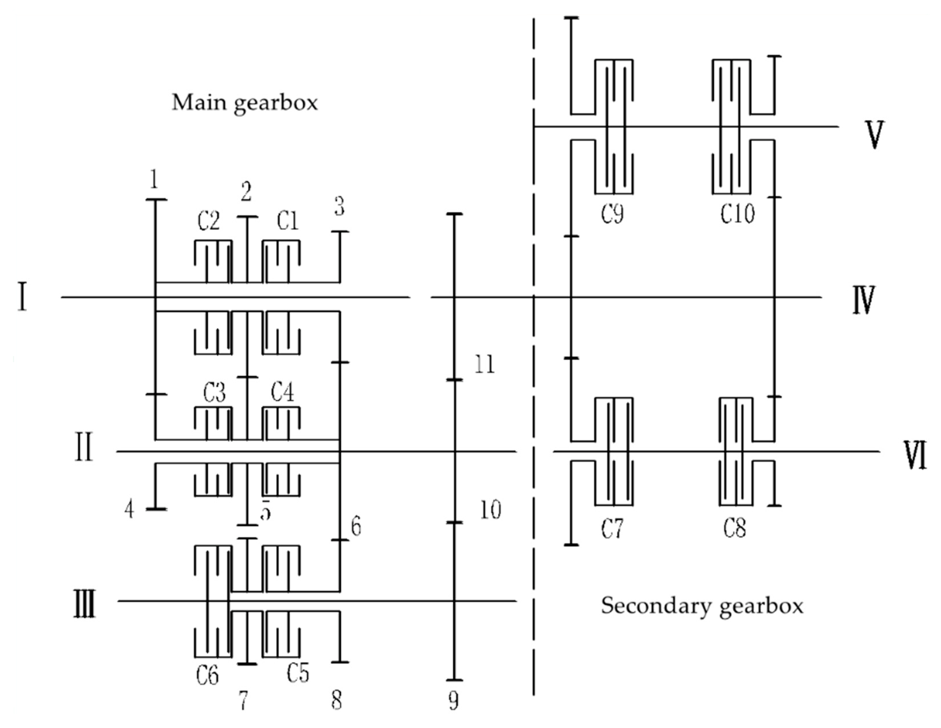
Figure 2.
Principle of electro-hydraulic control of power shift transmission.

Figure 3.
Structure diagram of shifting proportional solenoid valve. 1. Adjusting screw; 2. Adjusting spring; 3. Valve sleeve; 4. Coil; 5. Armature; 6. Valve body; 7. Valve baffle; 8. Spool; 9. Oil inlet ball valve.
Figure 3.
Structure diagram of shifting proportional solenoid valve. 1. Adjusting screw; 2. Adjusting spring; 3. Valve sleeve; 4. Coil; 5. Armature; 6. Valve body; 7. Valve baffle; 8. Spool; 9. Oil inlet ball valve.
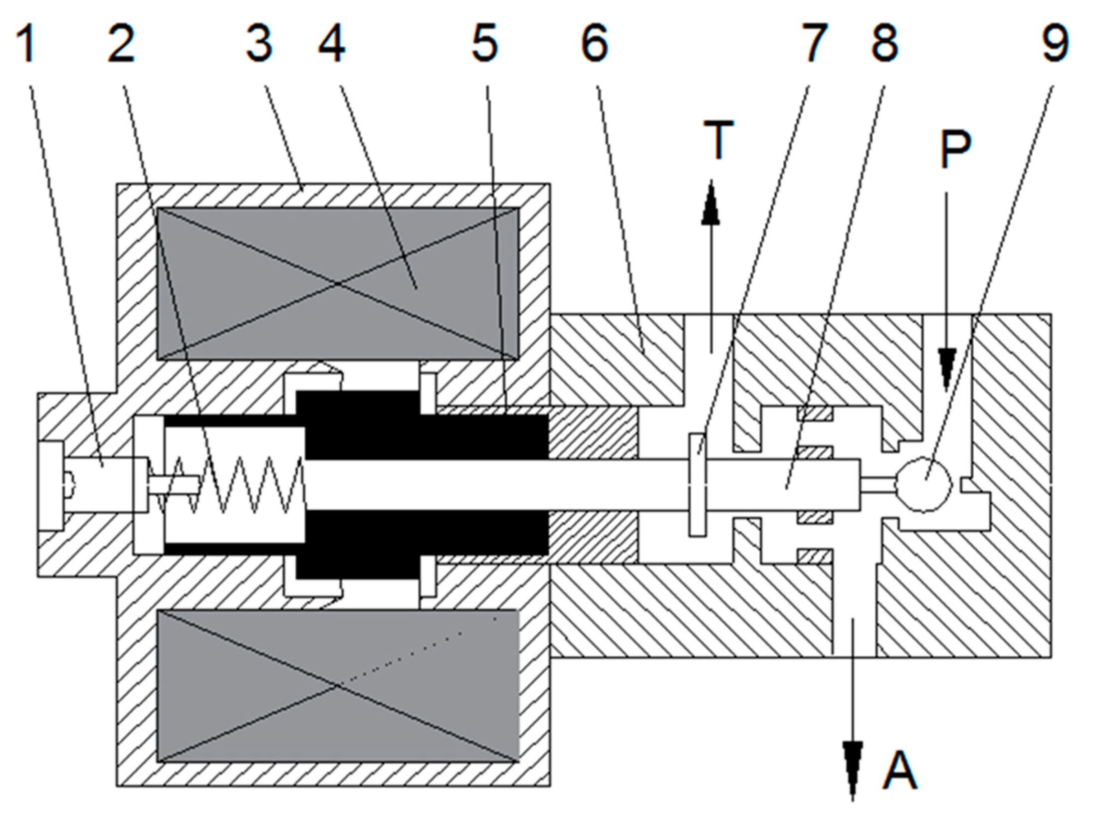
Figure 4.
Input current signal of proportional electromagnet.
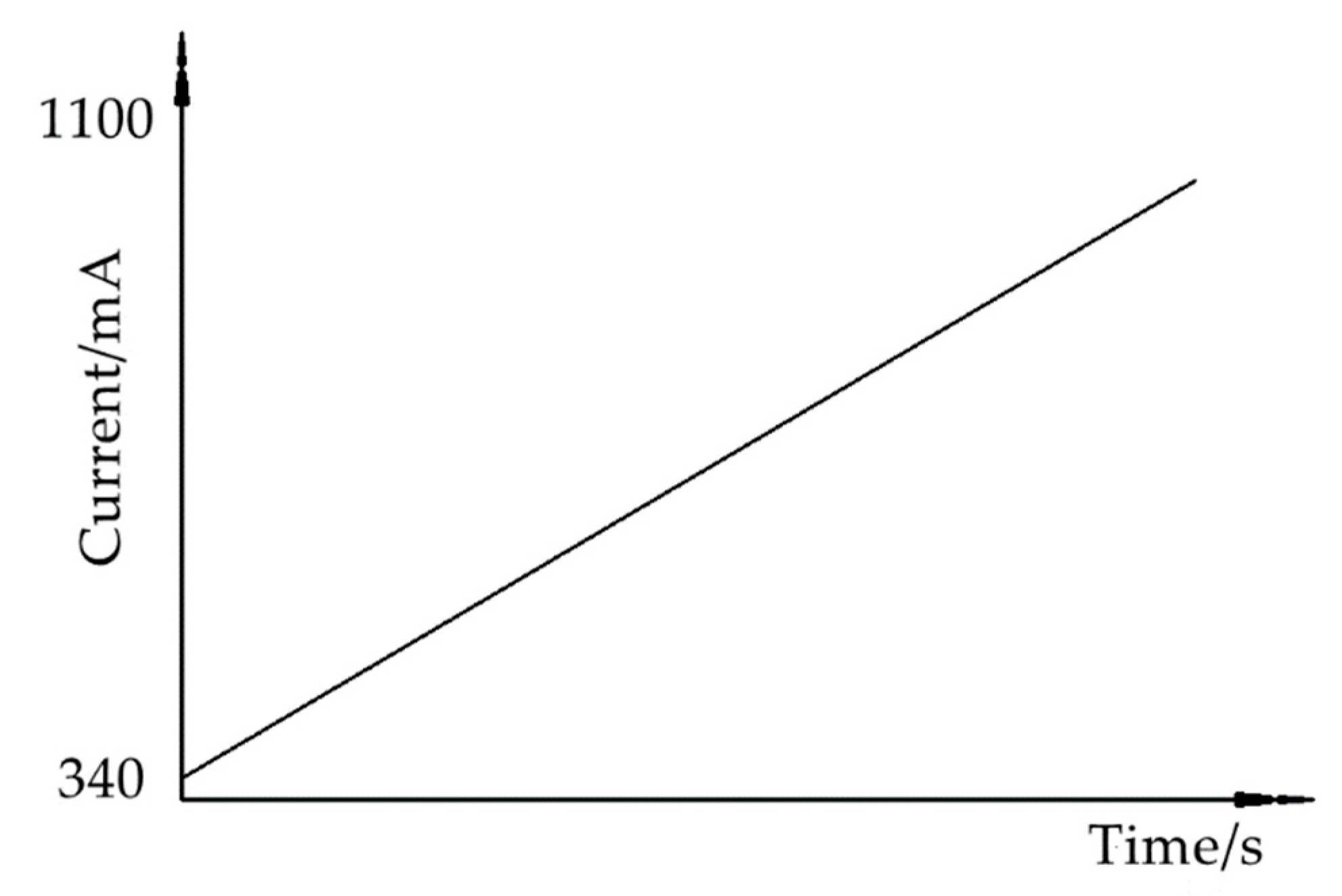
Figure 5.
PST control principle.
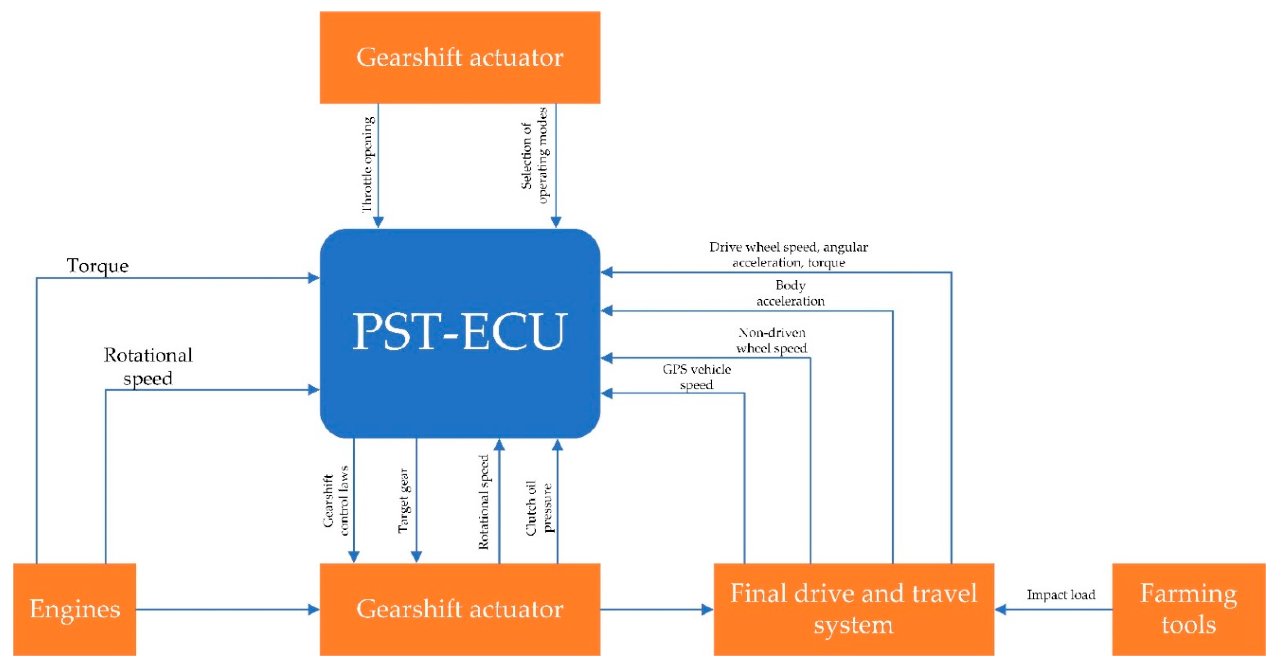
Figure 6.
Power shift process.

Figure 7.
Flow characteristics of faults mode. (a) Flow characteristics of leak mode. (b) Flow characteristics of blockage mode.
Figure 7.
Flow characteristics of faults mode. (a) Flow characteristics of leak mode. (b) Flow characteristics of blockage mode.
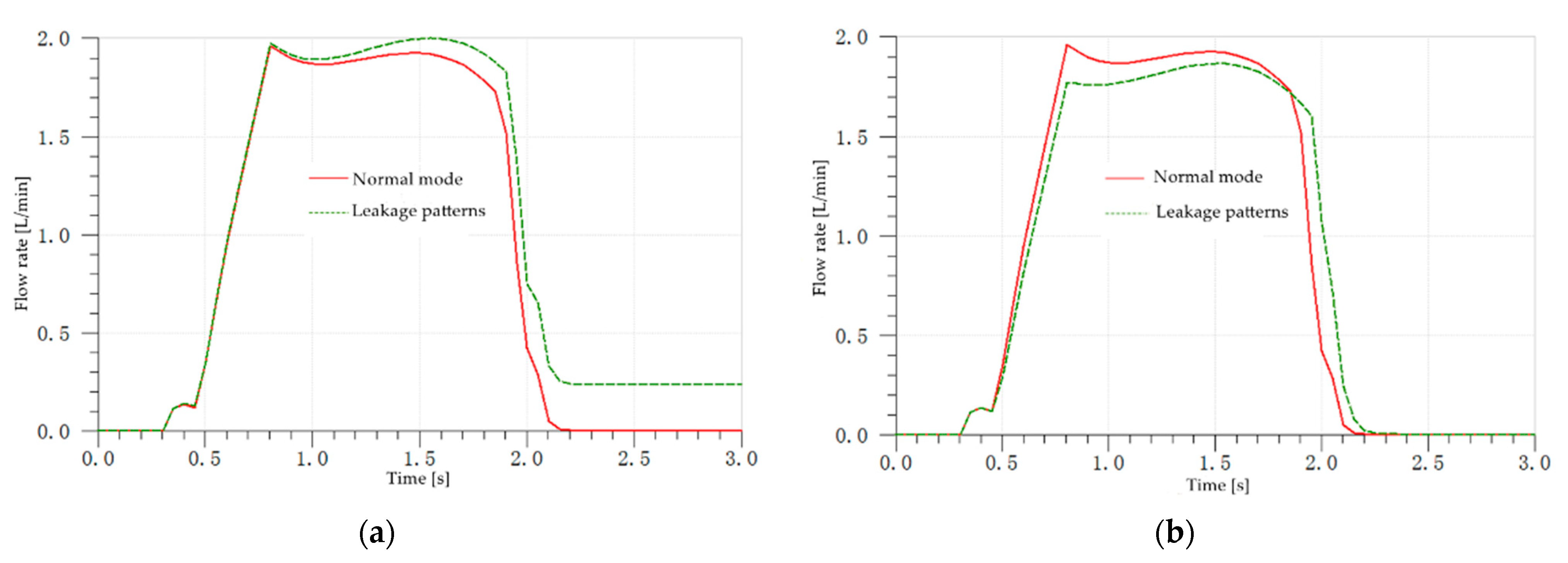
Figure 8.
Block diagram of fault diagnosis of PST electro-hydraulic system based on CAN bus.

Figure 10.
Mapping function of Gaussian kernel function.
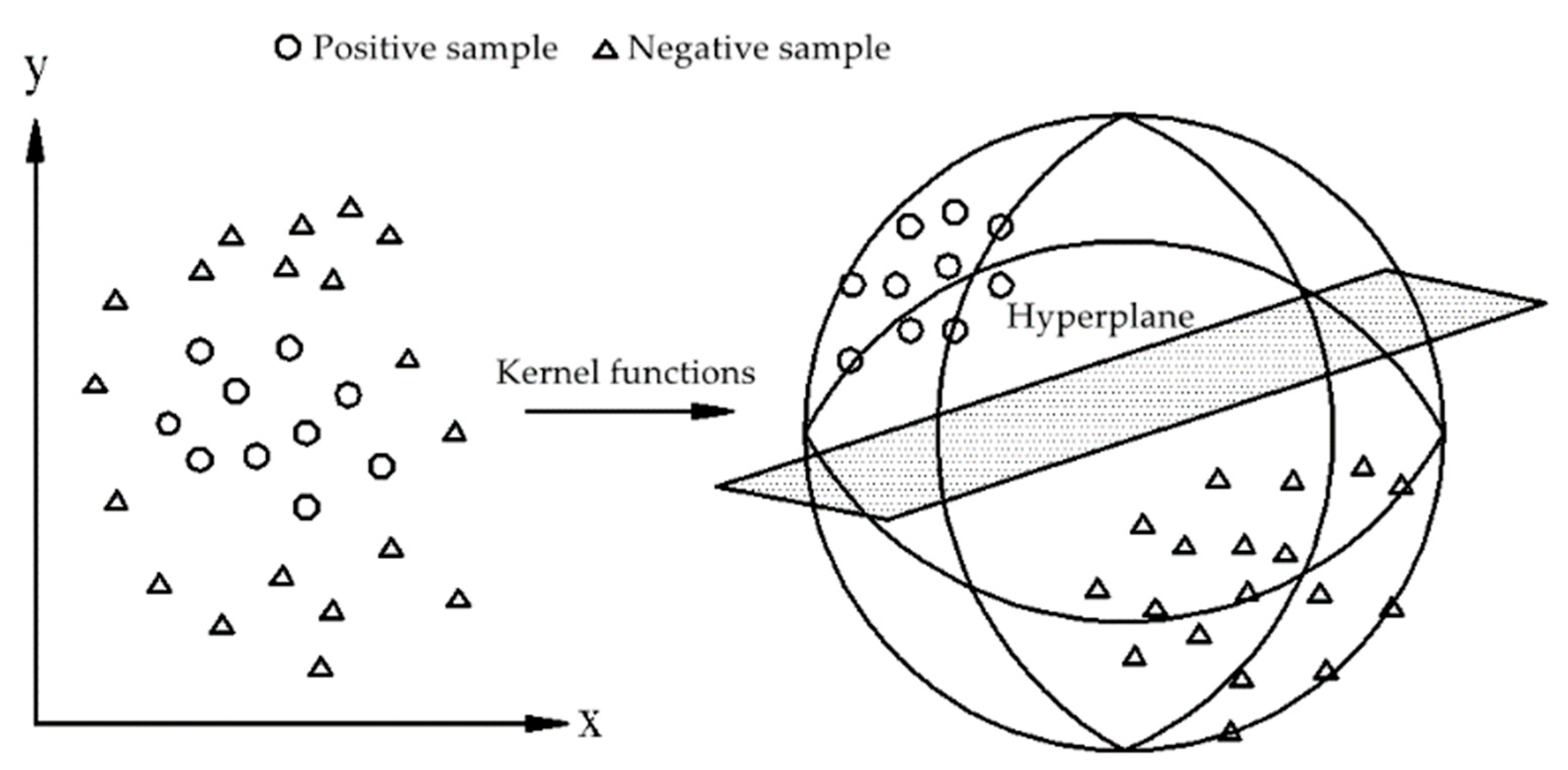
Figure 11.
Test sample data classification results.
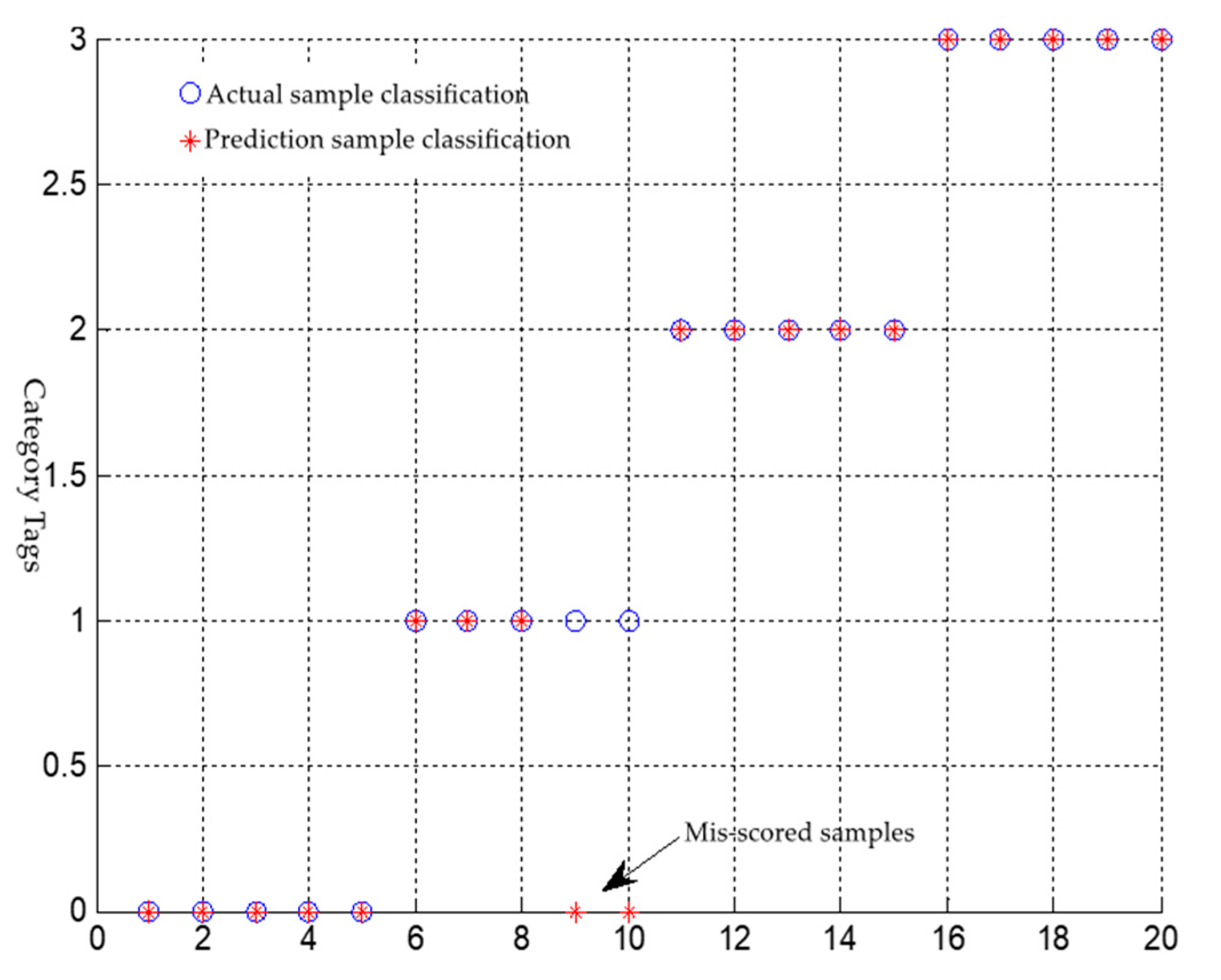
Figure 12.
All sample prediction classification results.


Table 1.
TCU electronic control system fault.
| Fault Category | Fault Specific Name |
|---|---|
| Sensor | Input shaft speed, output shaft speed sensor, shift clutch position sensor, gear position sensor, oil source pressure sensor, etc. |
| Electronic control unit | Program run away |
| Electronic control element circuit | Solenoid valve failure, solenoid valve drive circuit failure, power failure, etc. |
| CAN communication | The Vehicle Controller Unit (VCU) cannot receive the TCU signal, a certain signal of the TCU is lost, the CAN bus is short-circuited to the ground/power supply, or the circuit is disconnected. |
Table 2.
Power shift wet clutch common fault and maintenance.
| Common Error | Cause of Issue | Maintenance Method |
|---|---|---|
| Low system pressure, normal clutch leakage | 1. The oil level in the transmission oil pan is too low. 2. The spring of the pressure-regulating valve of the transmission control system is broken. 3. The spool of the pressure regulating valve is stuck. 4. The oil charge pump is working abnormally. | 1. Pour in the appropriate amount of oil. 2. Replace the spring on the pressure regulating valve. 3. Clean the spool and sleeve of the pressure regulating valve. 4. Examine and repair the charge pump. |
| Low system pressure and excessive clutch leakage | 1. The piston seal of the clutch cylinder is damaged or severely worn. 2. The oil seal at the connection between the clutch outer drum and the shaft is worn or damaged. 3. The oil pump works abnormally. | 1. Changing the sealing ring. 2. Changing the oil seal. 3. Replace or repair. |
| Transmission overheating | 1. The oil seal in the torque converter is worn, and the oil drain is too large. 2. The oil pump is worn. 3. The oil level in the transmission oil pan is too low. 4. The oil pump inlet line enters the air. | 1. Replacing the oil seal. 2. Oil pump replacement. 3. Increasing the quantity of oil. 4. Inspect the oil inlet pipe joint and tighten it. |
| Transmission is noisy | 1. The pump wheel is severely worn. 2. The oil pump is worn. 3. The bearing is severely worn or damaged. | 1. Changing the pump wheel. 2. Changing the oil pump. 3. Inspect the new bearing and replace it if necessary. |
| Low flow through cooler and low torque converter inlet pressure | 1. Torque converter safety valve spring is damaged. 2. A portion of the torque converter safety valve is opened. 3. The leakage in the torque converter is large. 4. The shift clutches oil seal is worn or damaged. | 1. Change the spring on the torque converter safety valve. 2. Examining the torque converter safety valve ball seat for wearing. 3. Inspect torque converter assembly parts and replace any that are severely worn. 4. Install a new clutch oil seal. |
| The flow through the cooler is small and the torque converter inlet pressure is high | 1. If the pressure of the gearbox lubricating oil is low, the cooler is blocked. 2. The oil return line of the cooler is partially blocked. 3. If the pressure of the gearbox lubricating oil is too high, the lubricating oil circuit is blocked. | 1. Vacuum the oil cooler. 2. Disinfect the oil return line. 3. Inspect transmission lubricating oil circuit and clear any clogged components. |
Table 3.
Combination encoding method.
| Classify | Distinguish |
|---|---|
| One against rest (OAR) | OAR is the earliest and most frequently used method at present. Its basic principle is to construct k second-class classifiers (k is the number of classes) by taking a certain class of samples as one class and other classes as another. Samples have to be discriminated against by k classifiers and output k classification values. The determination of this method is that the number of training samples is large, and the calculation is complicated. |
| One against one (OAO) | The basic idea behind OAO is to create one SVM classifier for two types of samples at the same time, so k (k − 1)/2 classifiers are required for the classification of k samples. When testing, each of the two types is compared, and the calculation is complicated. In addition, there is a problem that the identical sample belongs to multiple types, and the classification accuracy is low. |
| Directed Acyclic Graph (DAG) | DAG is part of the extension of OAO. The distinction is located between the prediction stage, which requires only k − 1 discriminant functions for each test, and the execution stage, which requires k − 1 discriminant functions for each test. It is fast in calculation and avoids the disadvantage of inseparable samples. |
| Binary Tree Multi-class Classification Algorithm | Combining the binary decision tree with SVM, the multi-class samples are divided into two categories from the root node, and the two sub-nodes continue to divide their samples into two categories, and then go down until each sub-node contains one category. Each node is classified by a support vector machine classifier, which has the advantage of fast classification speed, but after a sample is disqualified at a certain node, the error will continue irreversibly. |
| Direct classification algorithm | The advantage of solving multi-class samples as a whole is that the number of constructed classifiers is small, but this method has no unified construction method, the training process is slow, and the classifier structure is complex. |
Table 4.
Sample data.
| Number | X | C | K | I | S | XP | Fault Type |
|---|---|---|---|---|---|---|---|
| 1 | 3.718150 | 1.632139 | 1.590318 | 2.580348 | 1.580960 | 13.51565 | T |
| 2 | 3.718159 | 1.632138 | 1.590307 | 2.579709 | 1.580570 | 12.59522 | T |
| 3 | 3.718169 | 1.632137 | 1.590282 | 2.578267 | 1.579688 | 13.51165 | T |
| 4 | 3.718181 | 1.632131 | 1.590258 | 2.576918 | 1.578867 | 13.50904 | T |
| 5 | 3.718202 | 1.632125 | 1.590208 | 2.574224 | 1.577222 | 13.50390 | T |
| 6 | 3.71822 | 1.632117 | 1.590165 | 2.571917 | 1.575816 | 13.49945 | T |
| 7 | 3.718262 | 1.632101 | 1.590082 | 2.567598 | 1.573186 | 13.49108 | T |
| 8 | 3.718278 | 1.632094 | 1.590050 | 2.565904 | 1.572154 | 13.48779 | T |
| 9 | 3.718323 | 1.632077 | 1.589977 | 2.562131 | 1.569859 | 13.48042 | T |
| 10 | 3.718379 | 1.632053 | 1.589894 | 2.557801 | 1.567229 | 13.47198 | T |
| 11 | 4.641408 | 1.308204 | 1.577676 | 1.361743 | 1.040926 | 8.232270 | F1 |
| 12 | 4.503738 | 1.348064 | 1.606603 | 1.425565 | 1.057490 | 8.814577 | F1 |
| 13 | 4.374942 | 1.387634 | 1.627415 | 1.497733 | 1.079342 | 9.403138 | F1 |
| 14 | 4.119849 | 1.473445 | 1.546716 | 1.635828 | 1.110206 | 10.30141 | F1 |
| 15 | 3.986659 | 1.522576 | 1.552947 | 1.756648 | 1.153734 | 10.73721 | F1 |
| 16 | 3.897091 | 1.557487 | 1.543815 | 1.870622 | 1.201051 | 11.49526 | F1 |
| 17 | 3.829932 | 1.584728 | 1.571876 | 1.988583 | 1.254842 | 11.92903 | F1 |
| 18 | 3.783049 | 1.604309 | 1.577237 | 2.106763 | 1.313190 | 12.33731 | F1 |
| 19 | 3.752768 | 1.617206 | 1.581351 | 2.219805 | 1.372617 | 12.67724 | F1 |
| 20 | 3.734874 | 1.624917 | 1.584432 | 2.322164 | 1.429097 | 12.94919 | F1 |
| 21 | 1.909045 | 1.032249 | 1.508721 | 1.032450 | 1.000194 | 2.479529 | F2 |
| 22 | 2.488536 | 1.094736 | 1.505060 | 1.154214 | 1.054331 | 6.068260 | F2 |
| 23 | 2.939103 | 1.285464 | 1.513321 | 1.594527 | 1.240429 | 10.45648 | F2 |
| 24 | 2.986767 | 1.456093 | 1.506423 | 2.011038 | 1.381119 | 11.75795 | F2 |
| 25 | 3.141969 | 1.459963 | 1.515589 | 2.058338 | 1.409856 | 12.32977 | F2 |
| 26 | 3.287192 | 1.513136 | 1.515163 | 2.162645 | 1.429247 | 12.45779 | F2 |
| 27 | 3.416444 | 1.539293 | 1.512336 | 2.294414 | 1.490563 | 12.93440 | F2 |
| 28 | 3.546686 | 1.540993 | 1.502323 | 2.297025 | 1.490613 | 12.94182 | F2 |
| 29 | 3.447888 | 1.628382 | 1.518066 | 2.557372 | 1.570499 | 13.39684 | F2 |
| 30 | 3.512039 | 1.629298 | 1.516488 | 2.575288 | 1.580612 | 13.47951 | F2 |
| 31 | 3.068556 | 1.992056 | 1.775022 | 1.230561 | 1.802556 | 13.50322 | F3 |
| 32 | 3.216002 | 1.965321 | 1.875665 | 1.235621 | 1.892003 | 13.65206 | F3 |
| 33 | 3.055541 | 2.065384 | 1.802653 | 1.236654 | 1.596455 | 13.56332 | F3 |
| 34 | 3.116501 | 2.105387 | 1.794685 | 1.240051 | 1.792058 | 13.47669 | F3 |
| 35 | 3.120565 | 1.869322 | 1.824625 | 1.189985 | 1.903255 | 13.50566 | F3 |
| 36 | 3.142652 | 1.956588 | 1.778062 | 1.239856 | 1.946623 | 13.51229 | F3 |
| 37 | 3.050289 | 1.899231 | 1.826452 | 1.236488 | 1.885236 | 13.53656 | F3 |
| 38 | 3.10036 | 2.135655 | 1.926565 | 1.424886 | 1.92556 | 13.30886 | F3 |
| 39 | 3.021056 | 2.056674 | 1.881202 | 1.232301 | 1.702314 | 13.59933 | F3 |
| 40 | 3.002123 | 2.092635 | 1.702188 | 1.24552 | 1.95956 | 13.55699 | F3 |
Table 5.
Fisher Criterion for F1–F3 and T-Mode Characteristic Variables.
| Model | X | C | K | L |
|---|---|---|---|---|
| F1 and T | 0.023192 | 0.021835 | 0.003533 | 0.093898 |
| F2 and T | 0.076661 | 0.017363 | 3.253002 | 0.031308 |
| F3 and T | 1.369812 | 0.245968 | 0.177200 | 6.105690 |
Table 6.
Diagnostic results of leakage faults in hydraulic cylinder working circuit of different size training samples.
Table 6.
Diagnostic results of leakage faults in hydraulic cylinder working circuit of different size training samples.
| Training Samples/Groups | C 1 | γ 2 | Support Vector/Each | Test Samples/Groups | Misdiagnosed Samples/Groups | Accuracy Rate/% |
|---|---|---|---|---|---|---|
| 6 | 32 | 0.0078125 | 5 | 20 | 2 | 90 |
| 10 | 1024 | 0.03125 | 8 | 20 | 2 | 90 |
| 15 | 512 | 0.5 | 14 | 20 | 2 | 90 |
| 20 | 2048 | 0.5 | 14 | 20 | 1 | 95 |
1 penalty coefficient. 2 a parameter of the kernel function.
Publisher’s Note: MDPI stays neutral with regard to jurisdictional claims in published maps and institutional affiliations. |
© 2022 by the authors. Licensee MDPI, Basel, Switzerland. This article is an open access article distributed under the terms and conditions of the Creative Commons Attribution (CC BY) license (https://creativecommons.org/licenses/by/4.0/).
Share and Cite
MDPI and ACS Style
Ni, H.; Lu, L.; Sun, M.; Bai, X.; Yin, Y. Research on Fault Diagnosis of PST Electro-Hydraulic Control System of Heavy Tractor Based on Support Vector Machine. Processes 2022, 10, 791. https://doi.org/10.3390/pr10040791
AMA Style
Ni H, Lu L, Sun M, Bai X, Yin Y. Research on Fault Diagnosis of PST Electro-Hydraulic Control System of Heavy Tractor Based on Support Vector Machine. Processes. 2022; 10(4):791. https://doi.org/10.3390/pr10040791
Chicago/Turabian StyleNi, Huiting, Liqun Lu, Meng Sun, Xin Bai, and Yongfang Yin. 2022. "Research on Fault Diagnosis of PST Electro-Hydraulic Control System of Heavy Tractor Based on Support Vector Machine" Processes 10, no. 4: 791. https://doi.org/10.3390/pr10040791
Note that from the first issue of 2016, this journal uses article numbers instead of page numbers. See further details here.