
Python in Chemistry: Physicochemical Tools


N. D. Zelinsky Institute of Organic Chemistry Russian Academy of Sciences, 47 Leninsky Prospekt, 119991 Moscow, Russia
*
Author to whom correspondence should be addressed.
Processes 2023, 11(10), 2897; https://doi.org/10.3390/pr11102897
Submission received: 10 September 2023
/
Revised: 27 September 2023
/
Accepted: 28 September 2023
/
Published: 30 September 2023
(This article belongs to the Section Chemical Processes and Systems)
Abstract
:The popularity of the Python programming language in chemistry is growing every year. Python provides versatility, simplicity, and a rich ecosystem of libraries, making it the preferred choice for solving chemical problems. It is widely used for kinetic and thermodynamic calculations, as well as in quantum chemistry and molecular mechanics. Python is used extensively for laboratory automation and software development. Data analysis and visualization in chemistry have also become easier with the libraries available in Python. The evolution of theoretical and computational chemistry is expected in the future, especially at intersections with other fields such as machine learning. This review presents tools developed for applications in kinetic, thermodynamic, and quantum chemistry, instruments for molecular mechanics, and laboratory equipment. Online courses that help scientists without programming experience adapt Python to their chemical problems are also listed.
1. Introduction
Python is a powerful general-purpose programming language that is widely used in Internet applications, software development, data science, machine learning, and natural science. It was implemented by Guido van Rossum in 1989. Python is classified as an interpreted programming language that automates most of the fundamental operations (such as memory management) performed at the processor level (“machine code”). Python is considered a higher-level language than, for example, C++, because of its expressive syntax (which is close to natural language in many cases) and its rich variety of built-in data structures such as lists, tuples, sets, and dictionaries.
The Python philosophy is based on open source and an evolving community. Its syntax is simple and easy to learn, and the written code runs on any platform (PC, servers, clusters, mobile phones, and even IoT devices). Among the available libraries are many packages for almost any task, and these packages can often be downloaded for free (as well as Python itself). All this increases the speed of development and the popularity of this language.
However, the intensity of Python’s development has a downside. Constant development has created problems with version compatibility. Python, being an interpretable high-level language, cannot be as fast and efficient as C++. In scientific tasks, it is leveled by the fact that some of the libraries used by Python are written in C++ and pre-compiled. In this case, Python acts as a scripting language that organizes the efficient operation of code compiled in C++.
The programming initially originated in science. Scientists wrote programs to simplify and automate scientific tasks. Today, scientific programming still allows to automate labor-intensive tasks, modify and update research results, ensure collaboration, and create and compare models. Thanks to the speed of calculations and computations, the intensive development of which is especially noticeable in 2000–2020, the development in science is sufficiently accelerated.
As programming evolved, new tasks and opportunities emerged, and programming became a separate industry. Then, after the formation of the industry of commercial software products, programming returned to science in a new form. Such a long and complex way has given rise to a wide variety of languages. Below are the languages that are often used in scientific works.
Fortran. In the 1950s, a team from International Business Machines Inc. (Armonk, NY, USA) led by John Backus created the Fortran language. Fortran was the first high-level language to become popular, especially in the domain of numerical and scientific computing. It was widely adopted due to its increased level of abstraction, which made it orders of magnitude more compact than assembly programs. This popularity encouraged the development of excellent optimizing compilers, making Fortran the language of choice for many demanding scientific applications. It has a large body of tested Fortran routines and good support for modular programming [1].
MATLAB. It is a scripting language developed by a computer science professor to save students from learning Fortran. MATLAB excels at linear algebra and has many scientific and engineering tools, such as simulations and controls. It is fairly ‘mathematical’ in its syntax, making it easier to learn if already immersed in the subject. It provides an IDE to smooth over some of the difficulties of introductory programming, but it is expensive and limited outside of math and engineering subject areas. MATLAB isn’t free.
Wolfram Language (Mathematica). Mathematica is a popular programming tool in chemical engineering that was developed to solve complex mathematical problems with as little coding as possible. It has nearly 5000 built-in functions covering all areas of technical computing and is integrated into the fully integrated Mathematica system. The Wolfram Language is uniquely easy to read, write, and learn, but it requires a license and is more expensive than MATLAB.
C and C++. Even for a simple job, writing C code involves high time and effort costs. C was designed to allow a programmer to control computer hardware at a very low level. Traditionally, Fortran and MATLAB [2] have been the languages of choice for scientific computing applications. Developing object-oriented code for complex mathematical models, such as biology, finance, and materials science, requires parallel computing and the development of a graduate-level course in C++ for Scientific Computing.
Julia. It is a high-level and simultaneously high-performance free programming language designed for mathematical computations. It is also effective for writing general-purpose programs. Thanks to JIT (just-in-time) compilation and built-in support for multithreading and distributed computing, programs written with Julia are almost as efficient as applications written in compiled languages. Julia can call and use functions from other languages, such as C, Python, and Java.
R. This is a highly specialized language, which is great for statistical tasks. Often, there is a need not only to get data but also to transform that data or to interact with other external interfaces. Such tasks are difficult to implement using R. It has many great data visualization packages, including those that are publication-quality by default and powerful for developing custom displays of data. However, it is less developed in terms of engineering tools and more geared towards statistics.
BASIC (Beginners’ All-purpose Symbolic Instruction Code), Visual Basic (VB), Visual Basic for Application (VBA). BASIC is a family of general-purpose programming languages designed for ease of use. It was created in 1963. Visual Basic is a third-generation event-driven programming language from Microsoft, first released in 1991 and declared a legacy in 2008.
Today, many calculations proceed in Microsoft Excel. Chemical engineers frequently use MS Excel in experiments [3] and calculations as it is ubiquitous, easy to use, contains all the experimental data, and displays them clearly within Excel. VBA brings to Excel extensibility and flexibility [4]; it can be plugged in as the calculations are needed, e.g., for linear algebra, ordinary differential equations, regression analysis, partial differential equations, mathematical programming methods, and the connection to external devices or interfaces.
Pascal. Pascal grew out of ALGOL, a programming language intended for scientific computing. In the 1960s, Dr. Niklaus Wirth of the Swiss Federal Institute of Technology published his specification for a highly structured language that resembled ALGOL in many ways. Pascal is free-flowing, unlike FORTRAN, and reads like a natural language, making it easy to understand the code written in it. Pascal became widely accepted at universities due to two events: the Educational Testing Service’s addition of a Computer Science exam and the release of the Turbo Pascal compiler for the IBM Personal Computer. Pascal became the de facto standard for programming on the PC, with advanced features such as DPMI, Turbo Vision, and object-oriented extensions.
Java. In 1995, Java gained widespread popularity with the inclusion of the Java Virtual Machine (JVM). In Science, BioJava [5] has become popular. The project aims to facilitate bioinformatics analysis by providing parsers, data structures, and algorithms to address common challenges in genomics, structural biology, ontologies, phylogenetics, and other areas.
This review is focused specifically on Python, as this language has become incredibly popular in the scientific community. The reasons for its popularity are described above, and if we evaluate it in numbers, it is growing exponentially. Figure 1 shows the explosive growth in the number of articles on topics related to chemistry and program development in Python (the main literature search for the review is collected by querying through SciFinder using these keywords). The decrease in the number of Python publications in 2023 is due to the incomplete year at the time of writing the review.
In chemistry, Python solves a lot of tasks, and the range of tasks is expanding every day. By categorizing these tasks into groups, it has been possible to identify a few sections, as follows: Physical chemistry tasks include thermodynamics, kinetic models, quantum chemistry, and molecular mechanics tools. Python has solutions for spectroscopic problems and is also used for solving problems related to material science. There are a number of chemoinformatics and medical problems (to be covered in another review).
Machine learning and data analysis are increasingly being integrated into chemistry research, and robust ML-based models are becoming more and more in demand [6]. The scope of ML is expanding, and known approaches are well described [7,8,9,10,11,12].
Many of these tools are available for free download and are designed as Python libraries or customized tools. There are also free educational courses that help enrich scientific projects available on the Internet.
It is to be expected that the science at the interface between programming and chemistry will continue its intensive development. The current state of development in Python for chemistry is discussed below.
2. Classical Physical Chemistry
Python is most widely used in various areas of physical chemistry. Theoretical physical chemistry requires many computational operations in any of its sections. Applications of Python in physical chemistry include thermodynamic and kinetic models, tools for quantum mechanical calculations and molecular mechanical modeling, as well as tools for solving spectroscopic problems.
2.1. Kinetic Models Based on Transition State Theory
The task of kinetics in physical chemistry is to determine the rate of reactions. The Arrhenius equation is widely known in kinetic chemistry. According to the Arrhenius equation, the rate constant of a chemical reaction depends on the absolute temperature, as follows:
where k—the rate constant, T—the absolute temperature, A—preexponential factor, Ea—the activation energy, and R—the universal gas constant.
There are some limitations to accurate calculations using kinetic equations. In the low-temperature range, the temperature dependence of the rate of processes often deviates from the linearity of Arrhenius plots, and statistical approaches are used to describe such processes—the theory of transition state (TST) [13,14,15,16,17,18,19,20,21,22,23]. TST is an excellent basis for understanding and predicting a wide range of kinetic processes with significant molecular complexity and deviation from the Arrhenius law. In this theory, the rate constant is defined as follows:
where G—the Gibbs energy of activation, kB—the Boltzmann constant, and h—Planck’s constant.
Transition state theory (TST) involves two steps: the electronic structure characterization of stationary points on the potential energy surface (PES), followed by the calculation of the rate constants. Obviously, the accuracy of the resulting rate constants depends on the quality of the electronic structure results and the kinetic theory assumptions used to estimate them. Despite this, TST is widely used to calculate rate constants for a wide range of chemical reactions, both in the gas phase and in solution, due to its simplicity and limited PES requirements [13].
There are various programs available for determining reaction kinetics using TST and its variants, including Transitivity, TAMkin, Eyringpy, RMG, Micki, and TUMME. They are presented in Table 1. These programs are designed to calculate the kinetics of chemical reactions and are based on Python. The first six software packages in Table 1 rely heavily on transition state theory (TST). However, all have their own features or specializations for specific tasks.
In [13], the original TST theory is supplemented with a special function of ‘Transitivity’. This makes it possible to determine the tendency of a reaction to proceed in terms of the inverse of the apparent activation energy.
It takes into account experimental and theoretical rate processes such as quantum tunneling, transport properties, and diffusion in the vicinity of phase transitions [13]. The activation energy is determined by the following formula:
The Transitivity function is defined as follows:
the function γ(β) (Transitivity function = 1/Ea(β), where β = 1/kBT, kB—Boltzmann constant, T—absolute temperature).
Transition state-based speed calculation (TST) is also possible based on the variational theory of transition state (VTST) [19,20,21] and Rice–Ramsperger–Kassel–Marcus theory (RRKM) [19,20,21]. The rate coefficient k(T) of the bimolecular reaction A + B + C + D is calculated as follows [19]:
where K is the tunneling coefficient, q†, qa, and qb refer to the partition function without energy and zero oscillatory contribution, ∆ is the reaction barrier including zero-point corrections, and V is the reference volume used to estimate the translational part of the partition function.
In the simple case, it is possible to calculate the rate constants of reactions in the gas phase [14,19] and in solution [14] on the basis of TST. However, advanced Transitivity [13] supports homogeneous [13], heterogeneous [13], and enzyme-catalyzed reactions [13].
The programs [13] rely on Collins-Kimball theory to account for diffusion limitations. The consideration of electron transfer processes is based on the Marcus theory [14].
Microkinetic modeling is a method used in chemical kinetics that takes into account all possible reaction pathways. In this approach, molecules are modeled as individual objects, and their behavior is described by considering their motion, interactions, and reactions with each other [15,16,17]. The microkinetic approach requires working with whole systems of reactions, which, on the one hand, increases the scale of application of the program but, on the other hand, increases the computational load. It allows solving kinetic problems of a wide range [16,17] and heterogeneous catalysis in particular [15].
To use TST [15], the reaction network (including intermediates) and reaction pathways must be determined. This is followed by the calculation of energy barriers using electronic structure calculations. The result of the calculation is used to determine rate constants using TST and the Eckart correction [15].
The tunneling correction in transition state theory (TST) is a factor that accounts for the quantum mechanical tunneling effect of reactions occurring even at activation energies below the energy barrier. Traditional transition state theory accounts for the Wigner [14,15,16,17,18,19] and Eckart [14,16,17,18,19] theorems of adjusting the rate constant by relating it to the statistical sum of the activated complex (including the rotational quantum numbers of reactants and products as well as the angular momentum). The recalculation of the reaction rate constant is performed by calculating the partition function for the reactants and transition state, as well as the effective height of the energy barrier.
Wigner’s tunneling correction theory assumes tunneling to occur mostly at the top of the reaction barrier and requires information on the imaginary frequency at the transition state. The Wigner transmission coefficient is obtained through the following equation [14]:
where kB—Boltzmann constant, T—temperature, h—Planck’s constant, ν‡—imaginary frequency at the transition state.
The unsymmetrical Eckart potential [14] provides an accurate representation of the barrier shape and is used to calculate the probability of tunneling, P(E), which is determined by the energy E of the reactants passing through the barrier.
Here, a1, a2, and d are calculated from relationships proposed by Johnston and Heicklen and Brown, and described in the article [14].
Deformed Transition-State Theory (d-TST) shows better results [13] than Wigner-Eckart. Therefore, the deformed Bell 35, Bell 58, and Skodje–Truhlar corrections are used to account for tunneling. These corrections are described in [13].
When other methods of correcting rate constants are not quite accurate or applicable, the Monte Carlo kinetic method is often used. It works by randomly selecting a reaction from a network of reactions and calculating its rate constant using TST or another method [15,19]. In this case, the probability of each reaction is calculated, taking into consideration the rate constant and reactant concentrations. It is used to model both homogeneous and heterogeneous reactions, including gas-phase reactions, surface reactions, and enzyme-catalyzed reactions [15].
The use of third-party code and interaction with other programs are both an advantage (speeding up code development, focusing on certain tasks, universality due to well-known libraries) and a disadvantage (dependence on other code). For the structures in the transition state, the kinetic approaches require the electronic structure output files from quantum chemistry programs (Gaussian [13,14,19], Molpro, ORCA, NWChem [14], Q-Chem [14,19], PySCF [14], VASP [15,19], ASE [15], ADF, CHARMM, CPMD, CP2K [19]). RMG (Arkane) [16,17,18] requires converged electronic structure computations performed by the user with a variety of supported software packages such as Gaussian, Molpro, Orca, TeraChem, Q-Chem, and Psi4.
The opposite situation also occurs; the code of these programs [13,19] is often used by other projects. FRIGUS [29] provides interfaces for solving the rate equations using the Transitivity code [13], while pMuTT [30] uses the TAMkin code [19] for some other tasks.
As part of the discussion of TST, VTST, and RRKM, it is worth mentioning the VULCAN project. This is an open-source project written in Python. VULCAN is specifically designed to model the kinetics and chemical composition of the atmosphere of exoplanets [23].
2.2. Other Kinetic Approaches
Besides classical TST, there are VTST, RRKM, REMD, and approaches based on datasets. [20,21,22,23,24,25,26,27,28]. The program packages considered above relied on different variants of the TST in their calculations. A number of programs [24,25,26,27,28] use their own approaches to calculate kinetics.
A modernization of TST is the variational transition state theory—VTST. This is another widely used method in computational chemistry, that offers a more accurate representation of chemical reactions compared to TST, including by taking into account quantum-mechanical tunnel effects. The main difference between TST and VTST is that TST assumes that the reaction proceeds along a single reaction coordinate, while VTST takes into account the possibility of multiple reaction coordinates. VTST can be complemented by SCT (Small Curvative Tunneling) [20,21], which takes into account the effect of tunneling. The corresponding equations are solved either by the CSE (chemically significant eigenmodes) method based on the analysis of the eigenvalues of the transition matrix, which describes the change in the probability of finding the system in each of its states within a certain time interval [20], or analytically [21].
Modeling of chemical kinetics is possible by generating analytic Jacobians [27] without reference to specific kinetic theories. Estimation of kinetic parameters is also possible using modern Bayesian inference methods [26] (a statistical measure), as well as by applying Markov chain Monte Carlo [21,26].
The described projects use different methods to account for tunneling effects in chemical reactions. The Eckart correction [20] assumes a one-dimensional reaction coordinate and uses a semi-classical approximation to calculate the tunneling correction factor. The Wigner correction [20] uses a more accurate quantum mechanical approach to calculate the tunneling correction factor. A combination of SCT [21] and VTST [21] is also used to account for quantum mechanical tunneling effects. For polymers, tunneling effects are taken into account through the ring polymer transmission coefficient, which is a dynamic factor in the Bennett-Chandler factorization [24]. It is possible that the use of the Hamiltonian-reservoir Replica Exchange indirectly accounts for tunneling effects [25].
Kinetic programs are not stand-alone projects. They rely on Gaussian [20,21,24], Orca [21], Polyrate [20], Molpro [24], and MOPAC [24] modules and use the compiled libraries Numpy, Numba, and MSTor [20]. MPI [20] is used to implement multiprocessor computing.
An online database of radical polymerization rate coefficients is available online [22], which provides reliable kinetic data. It has a wide range of chemical reactions, including ion-molecular, neutral, and electron-molecular reactions.
The least standard approach is used in the development of the SIR (susceptible-infected-removed) model [28]. Using the analogy of virus spread, the use of kinetic models is explained. In this case, they used a second-order autocatalytic process and a SIR model to illustrate the dynamics of infection.
Summarizing the kinetic models, it can be concluded that the main emphasis is on the transition state theory. However, projects using their own approaches have also been developed. Kinetic projects rely extensively on already-written libraries, and their work often requires input data on electronic structures from other programs. Dependence on other libraries and programs increases the speed of development; the use of already-known program codes promotes wide distribution and rapid adaptation of these programs, although at the expense of their independence. Some programs lack a graphical interface, which is not a problem for experienced users but makes it difficult for scientists unfamiliar with programming.
2.3. Thermodynamic Models
Thermodynamic models are also common among Python developments. Table 2 shows some software packages that can provide various calculations of the thermodynamic properties of individual systems, individual system components (substances), or reaction characteristics.
Many projects for calculating thermodynamic quantities are based on density-functional theory (DFT) [30,31,32,33,34]. DFT is a quantum mechanical method that is used to predict the electronic structure and energy of molecules and materials. DFT uses electron density instead of a wave function to describe the state of the system. This reduces the number of coordinates calculated; instead of 3N coordinates (3 spatial coordinates for each of the N electrons), only three spatial coordinates of the electron density function are calculated. Obviously, this reduces the requirements for computational resources. This method is often used to calculate the electronic structures of molecules, binding energies, and molecular properties, which is useful in solid-state physics or chemistry.
The results of DFT calculations allow for the calculation of thermodynamic quantities such as energy, enthalpy, and heat capacity by methods of statistical mechanics [19,30,31,32,33]. Basically, statistical mechanics uses partition functions (q) to compute such quantities, which can be expressed as follows [30]:
where εi is the energy of state i, k is the Boltzmann constant, and T is the temperature.
For indistinguishable systems, Q(T, V, N) = qN/N! and energy (U), enthalpy (H), and heat capacity (C, constant volume) are expressed as follows [30]:
The rest are semi-empirical/empirical methods (including UNIFAC and SRK) [38] and approaches based on machine learning models and datasets [16,17,18,35], which are essentially state-of-the-art tools in empirical data processing. The list of programs based on DFT is shown in Table 2.
In theoretical approaches, thermochemical properties are mainly obtained by calculating the molecular partition function. The calculation of this function is based on the results of energy and electronic configuration calculations by the DFT method. Based on DFT calculations, thermochemical properties (heat of bond formation and dissociation energy) are calculated [19]. In some cases, DFT calculations are run in the program itself [32].
The calculation of the molecular partition function can be complemented by the calculation of vibrational frequencies and modes [19,30,33]. NMA (normal mode analysis) allows for the determination of vibrational frequencies [19,30], which opens up the possibility of analyzing vibrational spectra. The quasiharmonic Debye model [33] allows for the calculation of thermal contributions to the formation enthalpy.
The calculation of the energy barrier and search for the transition state of the reaction can be carried out by the method of “elastic tape with friction” (NEB) [31]. There are three implementations: NEB, CI-NEB, and AutoNEB [31]. These implementations do not require significant computational resources but can easily interface with any DFT code. The DFT is only required to calculate the total energy and forces acting on the system of atoms. NEB then assumes an initial path and converges to a “test” path in the potential energy in the neighborhood of the initial path.
TAMkin, pMuTT, Pasta, ASE, and AFLOW-CCE [19,30,31,32,33] are purely theoretical—ab initio approaches. They allow one to calculate the electronic configurations and thermodynamic properties of molecules. However, they require the results of DFT calculations, which require significant computational resources. A set of publicly available databases with the results of DFT calculations (OC20 Dataset and Community Challenges [35], RMG [16,17,18], pGrAdd [36], PYroMat [37], ETM [38]) allows to economize resources and use these calculations by many scientists. Additionally, the availability of a large amount of experimental data obtained using the ab initio approach allows for analyzing these data and identifying patterns. If the results are formed on the basis of the DFT method, then the search for formulas or other ways to reflect the patterns found in these data is similar to the empirical approach, but with the difference that the data are formed on the basis of theoretical calculations.
In contrast to the model-based projects discussed below, OC20 [35] presents a dataset (1.3 million) with over one million results from DFT calculations covering a variety of materials, surfaces, and adsorbates. It is not a model but is intended to provide data for machine learning models to help in the search and optimization of catalysts.
Instead of DFT, experimental data sets can be used [16,17,18,36,37]. Eigendata sets include kinetic and thermodynamic parameters obtained from real experimental data (including group values). The parameters and data are used for extrapolation or summarization (pGrAdd) to obtain the desired thermodynamic value. In the case of PYroMat [37], the dataset consists of 1000 models, each of which describes the thermodynamic properties and equilibria of a known compound (mainly gases).
Some approaches to calculating thermodynamic properties are based on the known UNIFAC and SRK models to describe the state of matter [38]. These models are part of the open-source Thermo library. UNIFAC and SRK are empirical approaches designed to predict the properties of substances based on empirical correlations and statistical data obtained from experiments. These methods take into account the chemical and physical features of substances and their interactions. As a result, empirical methods can provide good results in describing and predicting the behavior of mixtures, but their accuracy may be limited, especially in cases where there is significant variability and inaccuracy in experimental data. To calculate thermodynamics (critical temperatures, critical pressures, acentric factors, formation enthalpies, and standard Gibbs free energies), the program connects to online databases such as Dortmund Data Bank [41] and Chemeo [42], where the properties are estimated.
There are theoretical approaches in the literature that use neither DFT nor the empirical approach (IFG [39] and The First Law [40]). Thermodynamic coefficients of ideal Fermi gas (IFG) mode [39] use analytical formulae (which have been expressed through the first and second derivatives of the Helmholtz free energy) for the thermodynamic description of the non-relativistic Fermi ideal gas. Another approach is based on the direct application of the first law of thermodynamics [40].
Obviously, the described programs are not completely independent. Almost all projects based on ab initio calculations require as input files the results of DFT calculations (e.g., Gaussian or Q-Chem [19]). Third-party programs used for calculations are shown in Table 2.
In addition to DFT, these projects interact with other projects or among themselves. pMuTT [30] uses TAMkin [19] to calculate kinetics. PGrAdd [36] uses pMuTT [30] for unit conversion, SMILES code, inference to empirical relations, and calculation of the microkinetic model. PGrAdd also includes RDKit code, iPython, NumPy, and other libraries [36].
Thus, to date, programs of this type can be divided into two groups—theoretical and empirical. Theoretical approaches based on statistical mechanics use partition functions derived from the electronic configuration of molecules. It can be improved by normal mode analysis. Empirical ones are based on classical (UNIFAC, SRK) and modern methods (machine learning and datasets) of predicting the behavior of systems. Many programs focus on the gas phase and catalysts; some are able to predict interphase behavior.
Thermodynamic projects are quite firmly linked to kinetic ones. They can use each other’s code. In addition, they often use already-known libraries to convert values or files. DFT calculations obtained in other programs are, in many cases, necessary for thermodynamic calculations.
3. Quantum Chemistry
3.1. Quantum Chemistry
Quantum chemistry allows ab initio calculations, i.e., purely theoretical calculations without reliance on experimental data. This is their undeniable advantage, as it eliminates the need for research design, conducting experiments with expensive reagents and equipment, collecting and accumulating data, analyzing these data, and then searching for or confirming a pattern. The main applications of Python are summarized in Figure 2.
On the other hand, theoretical procedures require significant computational resources. In this regard, many program projects based on Python use this language for high-level tasks, otherwise as a scripting language. For repeatedly performed and practiced mathematical operations, libraries written in the productive and efficient C++ language are used. The inclusion of C++ libraries is “seamless” with the help of translation libraries [43]. For example, QFORTE [44] and PyBEST [45] rely on Pybind11, while Psi4NumPy uses NumPy [46]. In addition, Psi4 [47,48,49] includes the LIBMINTS library for computing tensors and matrices, which also opens the way to parallel computation.
Among the problems to be solved by the projects under consideration is the calculation of the molecular electronic structure. This mainly requires the result of DFT calculations (PySCF [50], dftatom [51], PSI4 [46,47,52], Molpro [53]). In this regard, several theories have been implemented in Python. The Self-Consistent Field (SCF) method is introduced for efficient Hartree-Fock [53] and Kohn–Sham DFT (KS-DFT) calculations with high performance in various chemical and electronic environments [46,47,52]. The density cumulant functional theory (DCFT) [46,47,52] is also presented.
In both HF and KS-DFT, the ground-state wavefunction is given as a single Slater determinant Φ0 of molecular orbitals ψ [46,47] with total electronic energy E:
Φ0 = A| ψ1(1) ψ2(2) … ψN(N)|
E = ⟨ Ψ0 | Ĥ | Ψ0 ⟩
The E energy should be minimized, subject to orbital orthogonality. This is equivalent to suggesting that electrons are independent particles that only interact with each other’s mean fields.
The minimization of the total energy within a given basis set leads to the following equation:
where C, E, and S are the matrices of the molecular orbital coefficients, a diagonal matrix of the corresponding eigenergies, and the atomic orbital overlap matrix, respectively.
FC = SCE
Then, the Fock matrix is defined as follows:
where T, V, J, and K are the kinetic energy matrix, the external potential, the Coulomb matrix, and the exchange matrix, respectively.
F = T + V + J + K
DCFT [46,47,52] provides a direct route to the calculation of molecular properties without the use of a wave function [46,47,52]. The energy is expressed in terms of the one- and two-particle density matrices (γ1 and γ2):
where and are the standard one- and two-electron integrals, and are the elements of γ1 and γ2, respectively.
To minimize the energy () [47], the equation needs to meet the N-representability conditions. γ2 is replaced in favor of its two-particle density cumulant with idempotent part k and a correction τ:
Molecular electronic structure can also be calculated without DFT based on unconventional wavefunction models with the pair Coupled-Cluster Doubles ansatz (pCCD) [45] or multideterminant wavefunction model [54]. The molecular electronic structure can also be calculated without DFT through variational and projection quantum eigensolvers, adaptive eigensolvers, quantum evolution of imaginary time, quantum Krylov methods, and quantum phase estimation [44].
Neural networks are already used in quantum chemistry. Similar to DFT, neural networks help solve the problem of fast and accurate prediction of the electronic properties of drug compounds [55]. They solve quantum problems such as computing the potential energy surface [56,57].
The development of computing power has opened new opportunities for resource-intensive computations. Today’s computational power allows us to perform much larger-scale computations and solve much more complex problems. As a result, there is a huge amount of data that needs to be processed. Routine processing of quantum-chemical calculation files requires thoroughness, considerable time, and attention. In this connection, various tools appear to facilitate the work. There appeared tools for working with the mathematical part [58,59,60], parsing the Gaussian outfile [61], calculating optimal scaling factors for the calculation of harmonic vibrational frequencies, fundamental vibrational frequencies, and zero vibrational energies from electronic structure calculations [62], and of eigenvalues of electronic symmetry [63]. A number of tools (FragBuilder [64] QMflow [65], QCforever [66], Dalton [67], PyADF [68]) are designed to configure, automate, and start calculations and can serve as independent calculation programs and as tool for launching more developed programs.
QChASM makes it possible to construct and manipulate complex molecular structures, perform routine tasks, and predict the results of selective homogeneous catalytic reactions [69].
Tools have been developed [61,70,71] for post-processing files of performed calculations of electronic structure and properties after the programs Gaussian, Molpro, Turbomole, Q-Chem, ORCA, NWChem, GAMESS-US, PSI4, and Tonto. In addition to tools, there are algorithms for extracting features from quantum computations and performing correlation analysis [72], and algorithms are presented for performing a topological analysis of an arbitrary function evaluated on an arbitrary grid of points [73].
There are online projects based on Python. WebProp was implemented as a web-based interface for assessing one-electron ab initio quality attributes [74]. The QCArchive (Quantum Chemistry Archive was created [75]) provides automatic computation and storage of quantum chemistry results. It provides free access to tens of millions of quantum chemistry calculations for machine learning, method validation, and force field fitting. QCARCHIVE realizes two goals: to generate reference results of calculations and to compute a standard set of DFT and MP2 methods using different basis sets, which can then be used for validation and comparison.
In assessing the level of sophistication of quantum chemistry applications developed in Python, we can conclude that they have evolved from single or few calculations to more complex workflows in which a number of interrelated computational tasks are performed. Today, this multi-scale modeling, combining different levels of accuracy, typically requires a large number of individual computations that depend on each other.
3.2. Spectroscopic Application
In analytical chemistry, it is often necessary to solve spectroscopic problems. Analysis and prediction of spectra simplifies the solution of analytical problems. The prediction of spectra is based on quantum mechanical or other theoretical calculations. The fields of Python application in spectroscopy are presented in Figure 3.
The most popular application of Python in this field is nuclear magnetic resonance spectra. Python has been used to develop chemistry modules for accurate and automatic calculation of NMR chemical shifts of small organic molecules using quantum chemical calculations [76] and prediction of amino acid type and secondary structure from correlated chemistry shifts [77].
There is a library based on machine learning for automatic identification of molecules from their NMR spectra [76]. A machine learning-based approach for analyzing several 2D HSQC (heteronuclear single quantum coherence) spectra [78] and their simulation based on the BMRB (Biological Magnetic Resonance Bank) database [79] has also been implemented.
The intersection of Python and NMR also finds application in biochemistry for determining local protein structure using NMR chemical shifts. In addition, Python has been used in optimizing protein structure studies [80,81,82] and RNA structure estimation in 13C [83].
Python also has applications in mass spectrometry [84], allowing peak matching [85], and MALDI-TOF MS [86]. Mass spectrometry adduct calculator to identify some adduct ions was created [87].
3.3. Molecular Mechanics
The method known as molecular mechanics uses the principles of classical mechanics to calculate the forces and energies present in molecular systems. Although molecules truly follow the rules of quantum mechanics, molecular mechanics allows the structure and relative energy of molecules to be accurately reproduced using the classical method. Molecular mechanics calculations are much faster than more complex ab initio calculations, so we can analyze larger molecular systems or large numbers of molecules. Moreover, molecular mechanics requires fewer computational resources to handle larger systems. Hybrid quantum-chemical and molecular-mechanical potentials can be used in the programs [93,94,95].
Machine learning is gradually being introduced into molecular mechanics projects. Models [96] based on neural networks and long-range forces (electrostatic and Van der waals forces) are emerging. ParFit [97] allows parameters for molecular mechanical calculations to be fitted with a neural network to match ab initio calculations.
Although molecular modeling methods are mature, they may not be optimal for complex systems and long timescales. Grand canonical methods [98] are integrated with OpenMM and provide optimized calculations at long times of molecular dynamics simulations, taking into account water molecules, which play a critical role in protein-drug interactions.
Rare events, whose probability of occurrence is low, are poorly handled by standard algorithms and require a huge amount of simulation time. To handle such events, GROMACS and CP2K need to be tuned to model rare events with unbiased dynamics [99], providing transition interface sampling and replica exchange transition interface sampling (RETIS). This approach allows one to study the chemical reactions and structural changes of compounds [99].
Similar to quantum-mechanical projects, a large amount of accumulated data requires preparation and further processing. There is a library [100] to set up the GROMACS/PLUMED input files for the calculation of dissociation-free energy. MDTraj [101], Wordom [102], and Pytim [103] allow one to work with trajectory data from molecular dynamics simulations. They work with GROMACS files, OpenMM, CHARMM, AMBER, etc. Pytim is mainly focused on the analysis of interfacial properties in molecular simulations.
4. Material Science
Materials science is an interdisciplinary science that studies the properties of materials in solid and liquid states. It includes the structure, electronic, thermal, chemical, magnetic, and optical properties of materials.
Computer modeling in materials science opens up the possibility of understanding the properties of materials at the molecular level. This allows scientists to predict material properties and optimize the structure of materials to obtain the desired properties. Often, materials are modeled with molecular dynamics [104].
Among the modeled properties are mechanical (strength, elasticity, plasticity, deformation characteristics), tribological properties (friction coefficients [104], adhesion [104] in lubricating monolayer films), thermodynamic properties (phase transitions, thermal conductivity, heat capacity, and temperature dependence of properties) [105,106,107], electronic properties (electrical conductivity, electropolarization, dielectric constant, and optical properties of materials) [106,107], and kinetic properties (diffusion).
Among semiconductor and insulating materials, the prediction of the thermodynamic properties of point defects has been widely developed. DFT calculations [107] and the supercell approach [106] are used to study such defects. Since these are resource-intensive problems, optimized approaches have emerged [106].
The properties of defects under study also include chemical potential [106], charge levels and electrostatic corrections [107], charged defect calculations with electrostatic correction, calculation of formation energies, and stability of point defects [107]. Such calculations can be performed for any materials [107] or specialized for specific ones, e.g., calculations of electrostatic potentials and fields of germanium detectors [108].
The range of applications in materials science is quite broad. Combined SCM (surface complexation models), DLVO (DLVO theory, named after Boris Derjaguin and Lev Landau, Evert Verwey, and Theodoor Overbeek) [109], and phase diagram calculations [34] can be performed. Application of Python in materials science allows screening in the chemical space of substances with required properties [104] and modeling of the properties of materials with different compositions [110]. It is possible to simulate the dynamics of chemical reactions and model the self-assembly of molecules into complex structures on surfaces [111].
In addition to calculations, tools have been developed to accelerate the setup, execution, post-processing, and analysis of calculations [107]. Tools have been developed to build structures [34,112], visualize, perform model calculations, and analyze simulated data [112], as well as analyze crystal structures [34].
Projects can both be quite independent as well as fully self-sufficient [109] and require libraries or output files. The RDKit library [104,111] is used for working with chemical structures, and the machine learning library scikit-learn [104,110] is used for data analysis. In some cases (DJMol [112]), the thermodynamic package discussed in Section 2 (Pymatgen [34]) is used for materials science modeling. The modeling may also require GROMACS [104] or VASP/Gaussian [34] molecular dynamics calculations, and results include the determination of friction coefficient, cohesive force, and nematic material [104].
5. Python in Software and Hardware
First of all, we should mention large-scale, multi-year projects that use Python. The well-known Avogadro project allows Python scripting [113]. Python in Avogadro is based on PyQt, which is a powerful and flexible tool for building graphical user interfaces. This means that users can write Python scripts to automate tasks, customize the interface, or add new features. Avogadro provides a set of ready-made Python plug-ins that allow users to interact with the Avogadro API and extend the functionality of the program.
Python plugins have been developed for reading and writing molecular data files, converting file formats, processing and matching molecular fingerprints, and working with SMARTS queries [114,115]. This opens up opportunities for integration with the OpenBabel toolkit, which facilitates chemoinformatics and provides a high-level Python interface for fast and efficient molecular data processing [114].
A Python tool called AutoVis [116,117] allows automatic color tracking and colorimetric titration with a webcam [118]. In some cases, the titration device is augmented with automatic pumps for pumping liquids, and the titration unit can be remotely controlled [119]. Similarly, the potentiometric instrument is for pH determination [120].
Python opens up possibilities for interfacing with single-board microcontrollers and microcomputers such as Arduino [121,122], Teensy [122], Raspberry Pi [123,124], or BeagleBone [122]. These devices are used to sub-connect to analytical equipment and read and process data. Arduino Uno [121] allows connecting USB devices to PC to collect data from various instruments: GC [125], capillary electrophoresis-UV, photometer, automated burettes, thermometers, pH meters, and thermocyclers for PCR [121]. A Raspberry Pi-based device with a connection to a spectrophotometer is assembled [123].
Data collection from the device and processing together with Arduino [125] are also carried out in gas chromatography [126]. In the case of thin-layer chromatography, a photo of the plate is taken using a smartphone. Then, based on a Python script, the analysis is performed in a three-dimensional space where red, green, and green colors are set to detect the pigment [127].
6. Educational Projects
With the development of digital technologies, students have the opportunity to acquire specific skills. These skills are in demand today and are likely to be an integral part of every advanced scientist’s education in the future. These are skills that combine the work of various disciplines at the interface of basic and practical sciences with the possibilities of computer technology.
Today, there are many courses that help to master such skills and familiarize chemistry students with the computer language Python. It is useful to list them.
Available courses include ways to predict physicochemical quantities (solubility, titration curves, calculation of distillation diagrams [128], calculation of entropy of a substance from specific heat and enthalpy data [129]), handling datasets [128], Fourier transform infrared spectroscopy [128], and NMR [128]. Courses teach modeling of first-order radioactive decay kinetics [129] using random number generators. They show calculations of the entropy of matter from specific heat capacity and enthalpy data and a nonlinear curve fitting to real gas data [129].
Python-based machine learning is gaining popularity in analytical chemistry, and many training courses in this direction are appearing. Machine learning is used in courses on NMR [130], visible spectrum spectrometry (Raspberry Pi-based spectrometer [131]), vibrational [132], and microwave [133,134] spectroscopy. The courses include training in obtaining and processing signals from analytical instruments [130,131,132,135], visualization [130], plotting, and linear approximation by the least-squares method. From the data obtained, one learns to calculate reaction rates [131], perform multiclass classification to determine functional groups (based on infrared absorption spectra [132]), and process test data [132].
In the last few decades, various aspects of quantum chemistry and molecular dynamics have been studied with the help of computer technology, in contrast to many other applied areas of chemistry. Therefore, this field has been described quite extensively, including in terms of educational projects. A training program for the solution of the Schrödinger equation has appeared: a three-point finite-difference numerical method to find the solutions and plot the results (wave functions or probability densities) for a particle in an infinite, finite, double finite, harmonic, Morse, or Kronig-Penney model [136]. There is a tutorial on estimating key parameters in the fitting procedure in the expression of the Slater orbital function in terms of a linear combination of Gaussian-type orbital functions [137]. Tutorials have been created on the iterative nature of the Hartree-Fock Procedure [133,134], determining structure from microwave spectroscopy, the calculation of accurate energies, and other aspects of theoretical chemistry [133,134], and Lennard-Jones fluid modeling [138]. Exercises in modeling and analyzing the dynamics of protein conformation under changes in temperature, solvation, and phosphorylation [139,140] to master the kinematic equations are provided.
Students are taught to solve mathematical problems in physical and analytical chemistry [141], including solving equations, Fourier transforms, calculating differentials and integrals, optimizing functions, working with complex numbers, vectors, matrices, and eigenvalues [141], as well as studying various aspects of the Boltzmann distribution [142]. An introduction to stochastic modeling of chemical and physical processes is presented [143] with detailed examples of stochastic modeling (Brownian motion, diffusion, chemical kinetics, and polymerization with chain growth).
Many training projects work with tools that have a web interface. For simplicity, they use Jupyter Notebooks [128,129,133,134,138,141,143,144,145]. Jupyter Notebook is an interactive, integrated development environment that provides the ability to create, execute, and document code, as well as share work results. It also includes functionality for quickly creating and displaying graphs, charts, and data visualizations. In addition, Jupyter Notebook provides the flexibility to modify and add code cells, text boxes, and images at any time. This allows the user to run code in real time and instantly view the results of the work. Jupyter Notebooks are popular in their use for teaching, but in addition to them, Excel is described in the courses [128].
7. Conclusions
Today, we are witnessing the rise of Python in the field of chemistry. Due to its simplicity and flexibility, Python is widely used for various computer tasks related to chemistry. Python is especially used for kinetic and thermodynamic calculations in physical chemistry. In kinetic physical chemistry, the emphasis on transition state theory is predominant, but projects have also been developed that use their own approaches. Kinetic packages often require input data on electronic structures from other programs. Thermodynamic projects are quite firmly linked to kinetic projects. Thermodynamic projects often require DFT calculations from other programs.
Python has many applications in quantum chemistry and molecular mechanics; it is one of the most growing areas of theoretical chemistry. In recent decades, research in quantum chemistry and molecular mechanics has been conducted mostly on computers, without real experiments. This is due to both the theoretical nature of the field and its increasing computational capabilities. Python itself is a scripting language that is often used for computations in conjunction with high-performing C++ libraries.
Python is actively used for laboratory automation, software development, and interfaces for laboratory equipment and instruments. It allows for simplified experiments, data collection, and instrument calibration. However, the application of the Python programming language itself for laboratory purposes is in its early stages at the level of trial projects. Obviously, this is due to the availability of ready-made commercial solutions, which are easier to purchase with a warranty, which eliminates the need for maintenance and responsibility on the part of the user. However, in areas that require a customized approach (e.g., high-cost equipment) and constant flexibility in equipment customization, hardware and software automation approaches may become in demand. In this case, it is desirable to create widely recognized standards and ready-made frameworks.
The Python programming language is becoming increasingly popular in the field of chemistry. This is due to its versatility, simplicity, and rich ecosystem of libraries and tools. Due to its accessibility and community support, Python is the preferred choice for solving a variety of chemistry problems and facilitating scientific research. However, dependence on other libraries and programs can both increase the speed of development, facilitate the use of existing code, and reduce the independence of those programs. In quantum chemistry, Python interacts with programs such as Gaussian, GAMESS, NWChem, and others to facilitate the automation of calculations, analysis of results, and complex simulations. It also opens the way to the use of DFT in physical chemistry for calculating the electron structure of a molecule and simulating spectra.
Data analysis and visualization is another area where Python has great potential. Libraries such as NumPy, Pandas, and Matplotlib allow one to efficiently process and analyze large amounts of data in chemistry. Working with such libraries is abundantly described in the many tutorials that currently exist. It is not appropriate to analyze these courses, but their availability allows everyone to find solutions to enrich their chemical research.
Undoubtedly, the development of theoretical and computational chemistry will continue in the future. Interesting intersections at the borders of different fields of chemistry are to be expected. Emerging combinations such as quantum chemistry and machine learning will be increasingly used in physical quantum chemistry, materials science, and other fields.
It is impossible to predict for sure which field will advance faster and more quickly and attract more research attention. These fields are all rapidly evolving in a variety of directions. We should anticipate the development of widespread, broadly accepted standards as the diversity of approaches increases.
Author Contributions
Conceptualization, F.V.R.; methodology, F.V.R.; validation, Y.E.R. and M.N.E.; formal analysis, F.V.R.; investigation, F.V.R.; data curation, Y.E.R. and M.N.E.; writing—original draft preparation, F.V.R.; writing—review and editing, Y.E.R. and M.N.E.; visualization, Y.E.R.; supervision, M.N.E. All authors have read and agreed to the published version of the manuscript.
Funding
This research received no external funding.
Data Availability Statement
Data are available from the authors on request.
Conflicts of Interest
The authors declare no conflict of interest.
References
- Chirila, D.B.; Lohmann, G. Introduction to Modern FORTRAN for the Earth System Sciences; Springer: Berlin/Heidelberg, Germany, 2015; ISBN 9783642370083. [Google Scholar]
- Pitt-Francis, J.; Whiteley, J. Guide to Scientific Computing in C++; Springer International Publishing: Cham, Switzerland, 2017; ISBN 9783319731315. [Google Scholar]
- Wong, K.W.W.; Barford, J.P. Teaching Excel VBA as a Problem Solving Tool for Chemical Engineering Core Courses. Educ. Chem. Eng. 2010, 5, e72–e77. [Google Scholar] [CrossRef]
- Kaess, M.; Easter, J.; Cohn, K. Visual Basic and Excel in Chemical Modeling. J. Chem. Educ. 1998, 75, 642. [Google Scholar] [CrossRef]
- Lafita, A.; Bliven, S.; Prlić, A.; Guzenko, D.; Rose, P.W.; Bradley, A.; Pavan, P.; Myers-Turnbull, D.; Valasatava, Y.; Heuer, M.; et al. BioJava 5: A Community Driven Open-Source Bioinformatics Library. PLoS Comput. Biol. 2019, 15, e1006791. [Google Scholar] [CrossRef] [PubMed]
- Artrith, N.; Butler, K.T.; Coudert, F.-X.; Han, S.; Isayev, O.; Jain, A.; Walsh, A. Best Practices in Machine Learning for Chemistry. Nat. Chem. 2021, 13, 505–508. [Google Scholar] [CrossRef] [PubMed]
- McKinney, W. Python for Data Analysis: Data Wrangling with Pandas, NumPy, and Ipython, 2nd ed.; O’Reilly Media: Sebastopol, CA, USA, 2018. [Google Scholar]
- McKinney, W. Data structures for statistical computing in python. In Proceedings of the 9th Python in Science Conference, Austin, TX, USA, 28 June–3 July 2010; Volume 445, pp. 51–56. [Google Scholar]
- Pérez, F.; Granger, B.E. IPython: A system for interactive scientific computing. Comput. Sci. Eng. 2007, 9, 21–29. [Google Scholar] [CrossRef]
- Perkel, J.M. Programming: Pick up Python. Nature 2015, 518, 125–126. [Google Scholar] [CrossRef] [PubMed]
- Rossant, C. Learning Ipython for Interactive Computing and Data Visualization; Createspace: Scotts Valley, CA, USA, 2015; ISBN 9781508599432. [Google Scholar]
- Morita, S. Chemometrics and Related Fields in Python. Anal. Sci. 2020, 36, 107–111. [Google Scholar] [CrossRef] [PubMed]
- Machado, H.G.; Sanches-Neto, F.O.; Coutinho, N.D.; Mundim, K.C.; Palazzetti, F.; Carvalho-Silva, V.H. “Transitivity”: A Code for Computing Kinetic and Related Parameters in Chemical Transformations and Transport Phenomena. Molecules 2019, 24, 3478. [Google Scholar] [CrossRef]
- Dzib, E.; Cabellos, J.L.; Ortíz-Chi, F.; Pan, S.; Galano, A.; Merino, G. Eyringpy: A Program for Computing Rate Constants in the Gas Phase and in Solution. Int. J. Quantum Chem. 2019, 119, e25686. Available online: https://www.theochemmerida.org/eyringpy (accessed on 25 September 2023). [CrossRef]
- Hermes, E.D.; Janes, A.N.; Schmidt, J.R. Micki: A Python-Based Object-Oriented Microkinetic Modeling Code. J. Chem. Phys. 2019, 151, 014112. [Google Scholar] [CrossRef]
- Gao, C.W.; Allen, J.W.; Green, W.H.; West, R.H. Reaction Mechanism Generator: Automatic Construction of Chemical Kinetic Mechanisms. Comput. Phys. Commun. 2016, 203, 212–225. [Google Scholar] [CrossRef]
- Dana, A.G.; Johnson, M.S.; Allen, J.W.; Sharma, S.; Raman, S.; Liu, M.; Gao, C.W.; Grambow, C.A.; Goldman, M.J.; Ranasinghe, D.S.; et al. Automated Reaction Kinetics and Network Exploration (Arkane): A Statistical Mechanics, Thermodynamics, Transition State Theory, and Master Equation Software. Int. J. Chem. Kinet. 2023, 55, 300–323. [Google Scholar] [CrossRef]
- Liu, M.; Grinberg Dana, A.; Johnson, M.S.; Goldman, M.J.; Jocher, A.; Payne, A.M.; Grambow, C.A.; Han, K.; Yee, N.W.; Mazeau, E.J.; et al. Reaction Mechanism Generator v3.0: Advances in Automatic Mechanism Generation. J. Chem. Inf. Model. 2021, 61, 2686–2696. [Google Scholar] [CrossRef] [PubMed]
- Ghysels, A.; Verstraelen, T.; Hemelsoet, K.; Waroquier, M.; Van Speybroeck, V. TAMkin: A Versatile Package for Vibrational Analysis and Chemical Kinetics. J. Chem. Inf. Model. 2010, 50, 1736–1750. Available online: https://molmod.github.io/tamkin/ (accessed on 25 September 2023). [CrossRef] [PubMed]
- Zhang, R.M.; Xu, X.; Truhlar, D.G. TUMME: Tsinghua University Minnesota Master Equation Program. Comput. Phys. Commun. 2022, 270, 108140. [Google Scholar] [CrossRef]
- Ferro-Costas, D.; Truhlar, D.G.; Fernández-Ramos, A. Pilgrim: A Thermal Rate Constant Calculator and a Chemical Kinetics Simulator. Comput. Phys. Commun. 2020, 256, 107457. Available online: https://comp.chem.umn.edu/pilgrim/ (accessed on 25 September 2023). [CrossRef]
- Van Herck, J.; Harrisson, S.; Hutchinson, R.A.; Russell, G.T.; Junkers, T. A Machine-Readable Online Database for Rate Coefficients in Radical Polymerization. Polym. Chem. 2021, 12, 3688–3692. [Google Scholar] [CrossRef]
- Tsai, S.-M.; Lyons, J.R.; Grosheintz, L.; Rimmer, P.B.; Kitzmann, D.; Heng, K. VULCAN: An Open-Source, Validated Chemical Kinetics Python Code for Exoplanetary Atmospheres. Astrophys. J. Suppl. Ser. 2017, 228, 20. [Google Scholar] [CrossRef]
- Suleimanov, Y.V.; Allen, J.W.; Green, W.H. RPMDrate: Bimolecular Chemical Reaction Rates from Ring Polymer Molecular Dynamics. Comput. Phys. Commun. 2013, 184, 833–840. Available online: https://greengroup.mit.edu/rpmdrate (accessed on 25 September 2023). [CrossRef]
- Fabregat, R.; Fabrizio, A.; Meyer, B.; Hollas, D.; Corminboeuf, C. Hamiltonian-Reservoir Replica Exchange and Machine Learning Potentials for Computational Organic Chemistry. J. Chem. Theory Comput. 2020, 16, 3084–3094. [Google Scholar] [CrossRef]
- Cohen, M.; Vlachos, D.G. Chemical Kinetics Bayesian Inference Toolbox (CKBIT). Comput. Phys. Commun. 2021, 265, 107989. [Google Scholar] [CrossRef]
- Niemeyer, K.E.; Curtis, N.J.; Sung, C.-J. PyJac: Analytical Jacobian Generator for Chemical Kinetics. Comput. Phys. Commun. 2017, 215, 188–203. Available online: https://slackha.github.io/pyJac/ (accessed on 25 September 2023). [CrossRef]
- Sucre-Rosales, E.; Fernández-Terán, R.; Carvajal, D.; Echevarría, L.; Hernández, F.E. Experience-Based Learning Approach to Chemical Kinetics: Learning from the COVID-19 Pandemic. J. Chem. Educ. 2020, 97, 2598–2605. [Google Scholar] [CrossRef]
- Coppola, C.M.; Kazandjian, M.V. Matrix Formulation of the Energy Exchange Problem of Multi-Level Systems and the Code FRIGUS. Rend. Lincei Sci. Fis. Nat. 2019, 30, 707–714. [Google Scholar] [CrossRef]
- Lym, J.; Wittreich, G.R.; Vlachos, D.G. A Python Multiscale Thermochemistry Toolbox (PMuTT) for Thermochemical and Kinetic Parameter Estimation. Comput. Phys. Commun. 2020, 247, 106864. Available online: https://vlachosgroup.github.io/pMuTT/ (accessed on 25 September 2023). [CrossRef]
- Kundu, S.; Bhattacharjee, S.; Lee, S.-C.; Jain, M. PASTA: Python Algorithms for Searching Transition StAtes. Comput. Phys. Commun. 2018, 233, 261–268. [Google Scholar] [CrossRef]
- Hjorth Larsen, A.; Jørgen Mortensen, J.; Blomqvist, J.; Castelli, I.E.; Christensen, R.; Dułak, M.; Friis, J.; Groves, M.N.; Hammer, B.; Hargus, C.; et al. The Atomic Simulation Environment—A Python Library for Working with Atoms. J. Phys. Condens. Matter 2017, 29, 273002. Available online: https://wiki.fysik.dtu.dk/ase/ (accessed on 25 September 2023). [CrossRef] [PubMed]
- Friedrich, R.; Esters, M.; Oses, C.; Ki, S.; Brenner, M.J.; Hicks, D.; Mehl, M.J.; Toher, C.; Curtarolo, S. Automated Coordination Corrected Enthalpies with AFLOW-CCE. Phys. Rev. Mater. 2021, 5, 043803. [Google Scholar] [CrossRef]
- Ong, S.P.; Richards, W.D.; Jain, A.; Hautier, G.; Kocher, M.; Cholia, S.; Gunter, D.; Chevrier, V.L.; Persson, K.A.; Ceder, G. Python Materials Genomics (Pymatgen): A Robust, Open-Source Python Library for Materials Analysis. Comput. Mater. Sci. 2013, 68, 314–319. Available online: https://pymatgen.org/ (accessed on 25 September 2023). [CrossRef]
- Chanussot, L.; Das, A.; Goyal, S.; Lavril, T.; Shuaibi, M.; Riviere, M.; Tran, K.; Heras-Domingo, J.; Ho, C.; Hu, W.; et al. Open Catalyst 2020 (OC20) Dataset and Community Challenges. ACS Catal. 2021, 11, 6059–6072. [Google Scholar] [CrossRef]
- Wittreich, G.R.; Vlachos, D.G. Python Group Additivity (PGrAdd) Software for Estimating Species Thermochemical Properties. Comput. Phys. Commun. 2022, 273, 108277. Available online: https://pypi.org/project/pgradd/ (accessed on 25 September 2023). [CrossRef]
- Martin, C.; Ranalli, J.; Moore, J. PYroMat: A Python Package for Thermodynamic Properties. J. Open Source Softw. 2022, 7, 4757. Available online: http://pyromat.org/ (accessed on 25 September 2023). [CrossRef]
- Cascioli, A.; Baratieri, M. Enhanced Thermodynamic Modelling for Hydrothermal Liquefaction. Fuel 2021, 298, 120796. [Google Scholar] [CrossRef]
- Kozharin, A.S.; Levashov, P.R. Thermodynamic Coefficients of Ideal Fermi Gas. Contrib. Plasma Phys. 2021, 61, e202100139. [Google Scholar] [CrossRef]
- Gajula, K.; Sharma, V.; Mishra, D.R.; Dumka, P. First Law of Thermodynamics for Closed System: A Python Approach. Res. Appl. Therm. Eng. 2022, 5, 1–10. [Google Scholar]
- DDBST—DDBST GmbH. Available online: http://www.ddbst.com (accessed on 16 August 2023).
- Cheméo. Available online: https://www.chemeo.com/ (accessed on 16 August 2023).
- Sun, Q.; Berkelbach, T.C.; Blunt, N.S.; Booth, G.H.; Guo, S.; Li, Z.; Liu, J.; McClain, J.D.; Sayfutyarova, E.R.; Sharma, S.; et al. Py SCF: The Python-based Simulations of Chemistry Framework. Wiley Interdiscip. Rev. Comput. Mol. Sci. 2018, 8, e1340. Available online: https://pyscf.org/ (accessed on 25 September 2023). [CrossRef]
- Stair, N.H.; Evangelista, F.A. QForte: An Efficient State-Vector Emulator and Quantum Algorithms Library for Molecular Electronic Structure. J. Chem. Theory Comput. 2022, 18, 1555–1568. Available online: https://github.com/evangelistalab/qforte (accessed on 25 September 2023). [CrossRef]
- Boguslawski, K.; Leszczyk, A.; Nowak, A.; Brzęk, F.; Żuchowski, P.S.; Kędziera, D.; Tecmer, P. Pythonic Black-Box Electronic Structure Tool (PyBEST). An Open-Source Python Platform for Electronic Structure Calculations at the Interface between Chemistry and Physics. Comput. Phys. Commun. 2021, 264, 107933. Available online: http://pybest.fizyka.umk.pl/ (accessed on 25 September 2023). [CrossRef]
- Smith, D.G.A.; Burns, L.A.; Sirianni, D.A.; Nascimento, D.R.; Kumar, A.; James, A.M.; Schriber, J.B.; Zhang, T.; Zhang, B.; Abbott, A.S.; et al. Psi4NumPy: An Interactive Quantum Chemistry Programming Environment for Reference Implementations and Rapid Development. J. Chem. Theory Comput. 2018, 14, 3504–3511. Available online: https://github.com/psi4/psi4numpy (accessed on 25 September 2023). [CrossRef]
- Turney, J.M.; Simmonett, A.C.; Parrish, R.M.; Hohenstein, E.G.; Evangelista, F.A.; Fermann, J.T.; Mintz, B.J.; Burns, L.A.; Wilke, J.J.; Abrams, M.L.; et al. Psi4: An Open-Source Ab Initio Electronic Structure Program: Psi4: An Electronic Structure Program. Wiley Interdiscip. Rev. Comput. Mol. Sci. 2012, 2, 556–565. Available online: https://psicode.org/ (accessed on 25 September 2023). [CrossRef]
- Parrish, R.M.; Burns, L.A.; Smith, D.G.A.; Simmonett, A.C.; DePrince, A.E., III.; Hohenstein, E.G.; Bozkaya, U.; Sokolov, A.Y.; Di Remigio, R.; Richard, R.M.; et al. Psi4 1.1: An Open-Source Electronic Structure Program Emphasizing Automation, Advanced Libraries, and Interoperability. J. Chem. Theory Comput. 2017, 13, 3185–3197. [Google Scholar] [CrossRef] [PubMed]
- Smith, D.G.A.; Burns, L.A.; Simmonett, A.C.; Parrish, R.M.; Schieber, M.C.; Galvelis, R.; Kraus, P.; Kruse, H.; Di Remigio, R.; Alenaizan, A.; et al. PSI4 1.4: Open-Source Software for High-Throughput Quantum Chemistry. J. Chem. Phys. 2020, 152, 184108. [Google Scholar] [CrossRef] [PubMed]
- Sun, Q.; Zhang, X.; Banerjee, S.; Bao, P.; Barbry, M.; Blunt, N.S.; Bogdanov, N.A.; Booth, G.H.; Chen, J.; Cui, Z.-H.; et al. Recent Developments in the PySCF Program Package. J. Chem. Phys. 2020, 153, 024109. [Google Scholar] [CrossRef] [PubMed]
- Čertík, O.; Pask, J.E.; Vackář, J. Dftatom: A Robust and General Schrödinger and Dirac Solver for Atomic Structure Calculations. Comput. Phys. Commun. 2013, 184, 1777–1791. [Google Scholar] [CrossRef]
- Mei, Y.; Yu, J.; Chen, Z.; Su, N.Q.; Yang, W. LibSC: Library for Scaling Correction Methods in Density Functional Theory. J. Chem. Theory Comput. 2022, 18, 840–850. [Google Scholar] [CrossRef] [PubMed]
- Werner, H.-J.; Knowles, P.J.; Manby, F.R.; Black, J.A.; Doll, K.; Heßelmann, A.; Kats, D.; Köhn, A.; Korona, T.; Kreplin, D.A.; et al. The Molpro Quantum Chemistry Package. J. Chem. Phys. 2020, 152, 144107. Available online: https://www.molpro.net/ (accessed on 25 September 2023). [CrossRef] [PubMed]
- Kim, T.D.; Richer, M.; Sánchez-Díaz, G.; Miranda-Quintana, R.A.; Verstraelen, T.; Heidar-Zadeh, F.; Ayers, P.W. Fanpy: A Python Library for Prototyping Multideterminant Methods in Ab Initio Quantum Chemistry. J. Comput. Chem. 2023, 44, 697–709. [Google Scholar] [CrossRef]
- Atz, K.; Isert, C.; Böcker, M.N.A.; Jiménez-Luna, J.; Schneider, G. Δ-Quantum Machine-Learning for Medicinal Chemistry. Phys. Chem. Chem. Phys. 2022, 24, 10775–10783. [Google Scholar] [CrossRef]
- Khorshidi, A.; Peterson, A.A. Amp: A Modular Approach to Machine Learning in Atomistic Simulations. Comput. Phys. Commun. 2016, 207, 310–324. [Google Scholar] [CrossRef]
- Dral, P.O. MLatom: A Program Package for Quantum Chemical Research Assisted by Machine Learning. J. Comput. Chem. 2019, 40, 2339–2347. [Google Scholar] [CrossRef]
- Tamayo-Mendoza, T.; Kreisbeck, C.; Lindh, R.; Aspuru-Guzik, A. Automatic Differentiation in Quantum Chemistry with Applications to Fully Variational Hartree–Fock. ACS Cent. Sci. 2018, 4, 559–566. [Google Scholar] [CrossRef] [PubMed]
- Kasim, M.F.; Lehtola, S.; Vinko, S.M. DQC: A Python Program Package for Differentiable Quantum Chemistry. J. Chem. Phys. 2022, 156, 084801. [Google Scholar] [CrossRef] [PubMed]
- Rubin, N.C.; DePrince, A.E., III. P†q: A Tool for Prototyping Many-Body Methods for Quantum Chemistry. Mol. Phys. 2021, 119, e1954709. [Google Scholar] [CrossRef]
- Nath, S.R.; Kurup, S.S.; Joshi, K.A. PyGlobal: A Toolkit for Automated Compilation of DFT-Based Descriptors: Software News and Updates. J. Comput. Chem. 2016, 37, 1505–1510. [Google Scholar] [CrossRef] [PubMed]
- Yu, H.S.; Fiedler, L.J.; Alecu, I.M.; Truhlar, D.G. Computational Thermochemistry: Automated Generation of Scale Factors for Vibrational Frequencies Calculated by Electronic Structure Model Chemistries. Comput. Phys. Commun. 2017, 210, 132–138. [Google Scholar] [CrossRef]
- Iraola, M.; Mañes, J.L.; Bradlyn, B.; Horton, M.K.; Neupert, T.; Vergniory, M.G.; Tsirkin, S.S. IrRep: Symmetry Eigenvalues and Irreducible Representations of Ab Initio Band Structures. Comput. Phys. Commun. 2022, 272, 108226. [Google Scholar] [CrossRef]
- Christensen, A.S.; Hamelryck, T.; Jensen, J.H. FragBuilder: An Efficient Python Library to Setup Quantum Chemistry Calculations on Peptides Models. PeerJ 2014, 2, e277. [Google Scholar] [CrossRef]
- Zapata, F.; Ridder, L.; Hidding, J.; Jacob, C.R.; Infante, I.; Visscher, L. QMflows: A Tool Kit for Interoperable Parallel Workflows in Quantum Chemistry. J. Chem. Inf. Model. 2019, 59, 3191–3197. [Google Scholar] [CrossRef]
- Sumita, M.; Terayama, K.; Tamura, R.; Tsuda, K. QCforever: A Quantum Chemistry Wrapper for Everyone to Use in Black-Box Optimization. J. Chem. Inf. Model. 2022, 62, 4427–4434. [Google Scholar] [CrossRef]
- Olsen, J.M.H.; Reine, S.; Vahtras, O.; Kjellgren, E.; Reinholdt, P.; Hjorth Dundas, K.O.; Li, X.; Cukras, J.; Ringholm, M.; Hedegård, E.D.; et al. Dalton Project: A Python Platform for Molecular- and Electronic-Structure Simulations of Complex Systems. J. Chem. Phys. 2020, 152, 214115. [Google Scholar] [CrossRef]
- Jacob, C.R.; Beyhan, S.M.; Bulo, R.E.; Gomes, A.S.P.; Götz, A.W.; Kiewisch, K.; Sikkema, J.; Visscher, L. PyADF—A Scripting Framework for Multiscale Quantum Chemistry. J. Comput. Chem. 2011, 32, 2328–2338. [Google Scholar] [CrossRef] [PubMed]
- Ingman, V.M.; Schaefer, A.J.; Andreola, L.R.; Wheeler, S.E. QChASM: Quantum Chemistry Automation and Structure Manipulation. Wiley Interdiscip. Rev. Comput. Mol. Sci. 2021, 11, e1510. [Google Scholar] [CrossRef]
- Hermann, G.; Pohl, V.; Tremblay, J.C.; Paulus, B.; Hege, H.-C.; Schild, A. ORBKIT: A Modular Python Toolbox for Cross-Platform Postprocessing of Quantum Chemical Wavefunction Data. J. Comput. Chem. 2016, 37, 1511–1520. [Google Scholar] [CrossRef] [PubMed]
- Hermann, G.; Pohl, V.; Tremblay, J.C. An Open-Source Framework for Analyzing N -Electron Dynamics. II. Hybrid Density Functional Theory/Configuration Interaction Methodology. J. Comput. Chem. 2017, 38, 2378–2387. [Google Scholar] [CrossRef] [PubMed]
- Mucelini, J.; Quiles, M.G.; Prati, R.C.; Da Silva, J.L.F. Correlation-Based Framework for Extraction of Insights from Quantum Chemistry Databases: Applications for Nanoclusters. J. Chem. Inf. Model. 2021, 61, 1125–1135. [Google Scholar] [CrossRef] [PubMed]
- Hutcheon, M.J.; Teale, A.M. Topological Analysis of Functions on Arbitrary Grids: Applications to Quantum Chemistry. J. Chem. Theory Comput. 2022, 18, 6077–6091. [Google Scholar] [CrossRef] [PubMed]
- Ganesh, V.; Kavathekar, R.; Rahalkar, A.; Gadre, S.R. WebProp: Web Interface Forab Initio Calculation of Molecular One-Electron Properties. J. Comput. Chem. 2008, 29, 488–495. [Google Scholar] [CrossRef] [PubMed]
- Smith, D.G.A.; Altarawy, D.; Burns, L.A.; Welborn, M.; Naden, L.N.; Ward, L.; Ellis, S.; Pritchard, B.P.; Crawford, T.D. The MolSSI QCA Rchive Project: An Open-source Platform to Compute, Organize, and Share Quantum Chemistry Data. Wiley Interdiscip. Rev. Comput. Mol. Sci. 2021, 11, e1491. [Google Scholar] [CrossRef]
- Yesiltepe, Y.; Nuñez, J.R.; Colby, S.M.; Thomas, D.G.; Borkum, M.I.; Reardon, P.N.; Washton, N.M.; Metz, T.O.; Teeguarden, J.G.; Govind, N.; et al. An Automated Framework for NMR Chemical Shift Calculations of Small Organic Molecules. J. Cheminform. 2018, 10, 52. [Google Scholar] [CrossRef]
- Fritzsching, K.J.; Yang, Y.; Schmidt-Rohr, K.; Hong, M. Practical Use of Chemical Shift Databases for Protein Solid-State NMR: 2D Chemical Shift Maps and Amino-Acid Assignment with Secondary-Structure Information. J. Biomol. NMR 2013, 56, 155–167. [Google Scholar] [CrossRef]
- Fino, R.; Byrne, R.; Softley, C.A.; Sattler, M.; Schneider, G.; Popowicz, G.M. Introducing the CSP Analyzer: A Novel Machine Learning-Based Application for Automated Analysis of Two-Dimensional NMR Spectra in NMR Fragment-Based Screening. Comput. Struct. Biotechnol. J. 2020, 18, 603–611. [Google Scholar] [CrossRef] [PubMed]
- Fucci, I.J.; Byrd, R.A. Nightshift: A Python Program for Plotting Simulated NMR Spectra from Assigned Chemical Shifts from the Biological Magnetic Resonance Data Bank. Protein Sci. 2022, 31, 63–74. [Google Scholar] [CrossRef] [PubMed]
- Fossi, M.; Linge, J.; Labudde, D.; Leitner, D.; Nilges, M.; Oschkinat, H. Influence of Chemical Shift Tolerances on NMR Structure Calculations Using ARIA Protocols for Assigning NOE Data. J. Biomol. NMR 2005, 31, 21–34. [Google Scholar] [CrossRef] [PubMed]
- Xiong, F.; Pandurangan, G.; Bailey-Kellogg, C. Contact Replacement for NMR Resonance Assignment. Bioinformatics 2008, 24, i205–i213. [Google Scholar] [CrossRef] [PubMed]
- Bhandari Neupane, J.; Neupane, R.P.; Luo, Y.; Yoshida, W.Y.; Sun, R.; Williams, P.G. Characterization of Leptazolines A–D, Polar Oxazolines from the Cyanobacterium Leptolyngbya Sp., Reveals a Glitch with the “Willoughby–Hoye” Scripts for Calculating NMR Chemical Shifts. Org. Lett. 2019, 21, 8449–8453. [Google Scholar] [CrossRef] [PubMed]
- Icazatti, A.A.; Martin, O.A.; Villegas, M.; Szleifer, I.; Vila, J.A. 13Check_RNA: A Tool to Evaluate 13C Chemical Shift Assignments of RNA. Bioinformatics 2018, 34, 4124–4126. [Google Scholar] [CrossRef]
- Ciach, M.A.; Miasojedow, B.; Skoraczyński, G.; Majewski, S.; Startek, M.; Valkenborg, D.; Gambin, A. Masserstein: Linear Regression of Mass Spectra by Optimal Transport. Rapid Commun. Mass Spectrom. 2021, e8956. [Google Scholar] [CrossRef] [PubMed]
- Letourneau, D.R.; Volmer, D.A. Constellation: An Open-Source Web Application for Unsupervised Systematic Trend Detection in High-Resolution Mass Spectrometry Data. J. Am. Soc. Mass Spectrom. 2022, 33, 382–389. [Google Scholar] [CrossRef]
- Parsons, L.M.; Cipollo, J.F. Assign-MALDI—A Free Software for Assignment of MALDI-TOF MS Spectra of Glycans Derivatized Using Common and Novel Labeling Strategies. Proteomics 2023, 23, 2200320. [Google Scholar] [CrossRef]
- Blumer, M.R.; Chang, C.H.; Brayfindley, E.; Nunez, J.R.; Colby, S.M.; Renslow, R.S.; Metz, T.O. Mass Spectrometry Adduct Calculator. J. Chem. Inf. Model. 2021, 61, 5721–5725. [Google Scholar] [CrossRef]
- Sibaev, M.; Crittenden, D.L. PyVCI: A Flexible Open-Source Code for Calculating Accurate Molecular Infrared Spectra. Comput. Phys. Commun. 2016, 203, 290–297. Available online: https://github.com/dlc62/pyvci (accessed on 25 September 2023). [CrossRef]
- Rehn, D.R.; Rinkevicius, Z.; Herbst, M.F.; Li, X.; Scheurer, M.; Brand, M.; Dempwolff, A.L.; Brumboiu, I.E.; Fransson, T.; Dreuw, A.; et al. Gator: A Python-driven Program for Spectroscopy Simulations Using Correlated Wave Functions. Wiley Interdiscip. Rev. Comput. Mol. Sci. 2021, 11, e1528. [Google Scholar] [CrossRef]
- Rinkevicius, Z.; Li, X.; Vahtras, O.; Ahmadzadeh, K.; Brand, M.; Ringholm, M.; List, N.H.; Scheurer, M.; Scott, M.; Dreuw, A.; et al. VeloxChem: A Python-driven Density-functional Theory Program for Spectroscopy Simulations in High-performance Computing Environments. Wiley Interdiscip. Rev. Comput. Mol. Sci. 2020, 10, e1457. [Google Scholar] [CrossRef]
- Lukin, S.; Užarević, K.; Halasz, I. Raman Spectroscopy for Real-Time and in Situ Monitoring of Mechanochemical Milling Reactions. Nat. Protoc. 2021, 16, 3492–3521. [Google Scholar] [CrossRef] [PubMed]
- Scheurer, M.; Reinholdt, P.; Kjellgren, E.R.; Haugaard Olsen, J.M.; Dreuw, A.; Kongsted, J. CPPE: An Open-Source C++ and Python Library for Polarizable Embedding. J. Chem. Theory Comput. 2019, 15, 6154–6163. [Google Scholar] [CrossRef] [PubMed]
- Field, M.J. The PDynamo Program for Molecular Simulations Using Hybrid Quantum Chemical and Molecular Mechanical Potentials. J. Chem. Theory Comput. 2008, 4, 1151–1161. Available online: https://www.pdynamo.org/ (accessed on 25 September 2023). [CrossRef] [PubMed]
- Martí, S. QMCube (QM 3): An All-purpose Suite for Multiscale QM/MM Calculations. J. Comput. Chem. 2021, 42, 447–457. Available online: https://github.com/sergio-marti/qm3 (accessed on 25 September 2023). [CrossRef]
- Lu, Y.; Farrow, M.R.; Fayon, P.; Logsdail, A.J.; Sokol, A.A.; Catlow, C.R.A.; Sherwood, P.; Keal, T.W. Open-Source, Python-Based Redevelopment of the ChemShell Multiscale QM/MM Environment. J. Chem. Theory Comput. 2019, 15, 1317–1328. [Google Scholar] [CrossRef]
- Yao, K.; Herr, J.E.; Toth, D.W.; Mckintyre, R.; Parkhill, J. The TensorMol-0.1 Model Chemistry: A Neural Network Augmented with Long-Range Physics. Chem. Sci. 2018, 9, 2261–2269. [Google Scholar] [CrossRef] [PubMed]
- Zahariev, F.; De Silva, N.; Gordon, M.S.; Windus, T.L.; Pérez García, M. ParFit: A Python-Based Object-Oriented Program for Fitting Molecular Mechanics Parameters to Ab Initio Data. J. Chem. Inf. Model. 2017, 57, 391–396. [Google Scholar] [CrossRef]
- Samways, M.L.; Bruce Macdonald, H.E.; Essex, J.W. Grand: A Python Module for Grand Canonical Water Sampling in OpenMM. J. Chem. Inf. Model. 2020, 60, 4436–4441. Available online: https://github.com/essex-lab/grand (accessed on 25 September 2023). [CrossRef] [PubMed]
- Lervik, A.; Riccardi, E.; van Erp, T.S. PyRETIS: A Well-Done, Medium-Sized Python Library for Rare Events. J. Comput. Chem. 2017, 38, 2439–2451. [Google Scholar] [CrossRef]
- Macchiagodena, M.; Karrenbrock, M.; Pagliai, M.; Procacci, P. Virtual Double-System Single-Box for Absolute Dissociation Free Energy Calculations in GROMACS. J. Chem. Inf. Model. 2021, 61, 5320–5326. [Google Scholar] [CrossRef] [PubMed]
- McGibbon, R.T.; Beauchamp, K.A.; Harrigan, M.P.; Klein, C.; Swails, J.M.; Hernández, C.X.; Schwantes, C.R.; Wang, L.-P.; Lane, T.J.; Pande, V.S. MDTraj: A Modern Open Library for the Analysis of Molecular Dynamics Trajectories. Biophys. J. 2015, 109, 1528–1532. Available online: https://www.mdtraj.org/ (accessed on 25 September 2023). [CrossRef] [PubMed]
- Seeber, M.; Felline, A.; Raimondi, F.; Muff, S.; Friedman, R.; Rao, F.; Caflisch, A.; Fanelli, F. Wordom: A User-Friendly Program for the Analysis of Molecular Structures, Trajectories, and Free Energy Surfaces. J. Comput. Chem. 2011, 32, 1183–1194. [Google Scholar] [CrossRef] [PubMed]
- Sega, M.; Hantal, G.; Fábián, B.; Jedlovszky, P. Pytim: A Python Package for the Interfacial Analysis of Molecular Simulations. J. Comput. Chem. 2018, 39, 2118–2125. [Google Scholar] [CrossRef] [PubMed]
- Summers, A.Z.; Gilmer, J.B.; Iacovella, C.R.; Cummings, P.T.; MCabe, C. MoSDeF, a Python Framework Enabling Large-Scale Computational Screening of Soft Matter: Application to Chemistry-Property Relationships in Lubricating Monolayer Films. J. Chem. Theory Comput. 2020, 16, 1779–1793. [Google Scholar] [CrossRef] [PubMed]
- Nkhwashu, M.I.; Moropeng, M.L.; Agboola, O.; Mavhungu, A.; Moropeng, R.C.; Fayomi, O.S.I. Modelling and Simulation of the Volume Flow of NH3, K2CO3 and MEA for the Carbon Dioxide Absorption from Coal. IOP Conf. Ser. Mater. Sci. Eng. 2021, 1107, 012060. [Google Scholar] [CrossRef]
- Arrigoni, M.; Madsen, G.K.H. Spinney: Post-Processing of First-Principles Calculations of Point Defects in Semiconductors with Python. Comput. Phys. Commun. 2021, 264, 107946. Available online: https://spinney.readthedocs.io/ (accessed on 25 September 2023). [CrossRef]
- Broberg, D.; Medasani, B.; Zimmermann, N.E.R.; Yu, G.; Canning, A.; Haranczyk, M.; Asta, M.; Hautier, G. PyCDT: A Python Toolkit for Modeling Point Defects in Semiconductors and Insulators. Comput. Phys. Commun. 2018, 226, 165–179. Available online: https://github.com/mbkumar/pycdt (accessed on 25 September 2023). [CrossRef]
- Li, J.; Liu, J.; Kooi, K. HPGe Detector Field Calculation Methods Demonstrated with an Educational Program, GeFiCa. Eur. Phys. J. C Part. Fields 2020, 80, 230. [Google Scholar] [CrossRef]
- Gil-Díaz, T.; Jara-Heredia, D.; Heberling, F.; Lützenkirchen, J.; Link, J.; Sowoidnich, T.; Ludwig, H.-M.; Haist, M.; Schäfer, T. Charge Regulated Solid-Liquid Interfaces Interacting on the Nanoscale: Benchmarking of a Generalized Speciation Code (SINFONIA). Adv. Colloid Interface Sci. 2021, 294, 102469. [Google Scholar] [CrossRef] [PubMed]
- Limami, H.; Guettioui, D.; Dahi, O.; Mehdi El Boustani, E.; Manssouri, I.; El Alami, A.; Khaldoun, A. Machine Learning Forecasting of Thermal, Mechanical and Physicochemical Properties of Unfired Clay Bricks with Plastic Waste Additives. Mater. Today 2023, 72, 3509–3513. [Google Scholar] [CrossRef]
- Clamons, S.; Qian, L.; Winfree, E. Programming and Simulating Chemical Reaction Networks on a Surface. J. R. Soc. Interface 2020, 17, 20190790. [Google Scholar] [CrossRef] [PubMed]
- Prasanna, K.G.; Sunil, R.; Gupta, K.; Lee, S.-C. DJMol: An Open-source Modeling Platform for Computational Chemistry and Materials Science with a Python Interpreter. J. Comput. Chem. 2021, 42, 2116–2129. Available online: https://djmolprogram.github.io/ (accessed on 25 September 2023). [CrossRef]
- Hanwell, M.D.; Curtis, D.E.; Lonie, D.C.; Vandermeersch, T.; Zurek, E.; Hutchison, G.R. Avogadro: An Advanced Semantic Chemical Editor, Visualization, and Analysis Platform. J. Cheminform. 2012, 4, 17. Available online: https://avogadro.cc/ (accessed on 25 September 2023). [CrossRef] [PubMed]
- O’Boyle, N.M.; Morley, C.; Hutchison, G.R. Pybel: A Python Wrapper for the OpenBabel Cheminformatics Toolkit. Chem. Cent. J. 2008, 2, 5. Available online: https://openbabel.org/ (accessed on 25 September 2023). [CrossRef]
- Verstraelen, T.; Adams, W.; Pujal, L.; Tehrani, A.; Kelly, B.D.; Macaya, L.; Meng, F.; Richer, M.; Hernández-Esparza, R.; Yang, X.D.; et al. IOData: A Python Library for Reading, Writing, and Converting Computational Chemistry File Formats and Generating Input Files. J. Comput. Chem. 2021, 42, 458–464. Available online: https://pypi.org/project/iodata/ (accessed on 25 September 2023). [CrossRef]
- Vargas, S.; Zamirpour, S.; Menon, S.; Rothman, A.; Häse, F.; Tamayo-Mendoza, T.; Romero, J.; Sim, S.; Menke, T.; Aspuru-Guzik, A. Team-Based Learning for Scientific Computing and Automated Experimentation: Visualization of Colored Reactions. J. Chem. Educ. 2020, 97, 689–694. [Google Scholar] [CrossRef]
- Duvvuri, H.; Wheeler, L.C.; Harms, M.J. Pytc: Open-Source Python Software for Global Analyses of Isothermal Titration Calorimetry Data. Biochemistry 2018, 57, 2578–2583. Available online: https://github.com/harmslab/pytc (accessed on 25 September 2023). [CrossRef]
- Tan, S.W.B.; Naraharisetti, P.K.; Chin, S.K.; Lee, L.Y. Simple Visual-Aided Automated Titration Using the Python Programming Language. J. Chem. Educ. 2020, 97, 850–854. [Google Scholar] [CrossRef]
- Yang, F.; Lai, V.; Legard, K.; Kozdras, S.; Prieto, P.L.; Grunert, S.; Hein, J.E. Augmented Titration Setup for Future Teaching Laboratories. J. Chem. Educ. 2021, 98, 876–881. [Google Scholar] [CrossRef]
- Jin, H.; Qin, Y.; Pan, S.; Alam, A.U.; Dong, S.; Ghosh, R.; Deen, M.J. Open-Source Low-Cost Wireless Potentiometric Instrument for PH Determination Experiments. J. Chem. Educ. 2018, 95, 326–330. [Google Scholar] [CrossRef]
- Grinias, J.P.; Whitfield, J.T.; Guetschow, E.D.; Kennedy, R.T. An Inexpensive, Open-Source USB Arduino Data Acquisition Device for Chemical Instrumentation. J. Chem. Educ. 2016, 93, 1316–1319. [Google Scholar] [CrossRef] [PubMed]
- Urban, P.L. Universal Electronics for Miniature and Automated Chemical Assays. Analyst 2015, 140, 963–975. [Google Scholar] [CrossRef] [PubMed]
- Chng, J.J.K.; Patuwo, M.Y. Building a Raspberry Pi Spectrophotometer for Undergraduate Chemistry Classes. J. Chem. Educ. 2021, 98, 682–688. [Google Scholar] [CrossRef]
- Navarre, E.C. Extensible Interface for a Compact Spectrophotometer for Teaching Molecular Absorption in the Undergraduate Laboratory. J. Chem. Educ. 2020, 97, 1500–1503. [Google Scholar] [CrossRef]
- Hinterberger, E.; Ackerly, E.; Chen, Y.; Li, Y.C. Development of a Low-Cost and Versatile Gas Chromatography System for Teaching Analytical Chemistry. J. Chem. Educ. 2021, 98, 4074–4077. [Google Scholar] [CrossRef]
- Green, M.; Chen, X. Data Functionalization for Gas Chromatography in Python. J. Chem. Educ. 2020, 97, 1172–1175. [Google Scholar] [CrossRef]
- Saldaña, M.; Valenzuela, S.A.; Moor, S.R.; Metola, P.; Anslyn, E.V. K-5 Thin-Layer Chromatography: Three-Dimensional Analysis of Pigments from Plant Materials Using an Interlocking Building-Block Photography Box. J. Chem. Educ. 2020, 97, 4414–4419. [Google Scholar] [CrossRef]
- Menke, E.J. Series of Jupyter Notebooks Using Python for an Analytical Chemistry Course. J. Chem. Educ. 2020, 97, 3899–3903. Available online: https://github.com/erik-menke/AnalyticalProjects (accessed on 25 September 2023). [CrossRef]
- Weiss, C.J.; Klose, A. Introducing Students to Scientific Computing in the Laboratory through Python and Jupyter Notebooks. In ACS Symposium Series: Teaching Programming across the Chemistry Curriculum; American Chemical Society: Washington, DC, USA, 2021; pp. 57–67. ISBN 9780841298194. [Google Scholar]
- Weiss, C.J. A Creative Commons Textbook for Teaching Scientific Computing to Chemistry Students with Python and Jupyter Notebooks. J. Chem. Educ. 2021, 98, 489–494. [Google Scholar] [CrossRef]
- Bougot-Robin, K.; Paget, J.; Atkins, S.C.; Edel, J.B. Optimization and Design of an Absorbance Spectrometer Controlled Using a Raspberry Pi to Improve Analytical Skills. J. Chem. Educ. 2016, 93, 1232–1240. [Google Scholar] [CrossRef]
- Thrall, E.S.; Lee, S.E.; Schrier, J.; Zhao, Y. Machine Learning for Functional Group Identification in Vibrational Spectroscopy: A Pedagogical Lab for Undergraduate Chemistry Students. J. Chem. Educ. 2021, 98, 3269–3276. [Google Scholar] [CrossRef]
- Fortenberry, R.C.; McDonald, A.R.; Shepherd, T.D.; Kennedy, M.; Sherrill, C.D. PSI4Education: Computational Chemistry Labs Using Free Software. In The Promise of Chemical Education: Addressing our Students’ Needs; American Chemical Society: Washington, DC, USA, 2015; pp. 85–98. ISBN 9780841230927. Available online: https://psicode.org/posts/psi4education/ (accessed on 25 September 2023).
- Magers, D.B.; Chávez, V.H.; Peyton, B.G.; Sirianni, D.A.; Fortenberry, R.C.; Ringer McDonald, A. PSI4EDUCATION: Free and Open-Source Programing Activities for Chemical Education with Free and Open-Source Software. In ACS Symposium Series: Teaching Programming across the Chemistry Curriculum; American Chemical Society: Washington, DC, USA, 2021; pp. 107–122. ISBN 9780841298194. [Google Scholar]
- van Staveren, M. Integrating Python into a Physical Chemistry Lab. J. Chem. Educ. 2022, 99, 2604–2609. [Google Scholar] [CrossRef]
- Srnec, M.N.; Upadhyay, S.; Madura, J.D. A Python Program for Solving Schrödinger’s Equation in Undergraduate Physical Chemistry. J. Chem. Educ. 2017, 94, 813–815. [Google Scholar] [CrossRef]
- Stewart, B.; Hylton, D.J.; Ravi, N. A Systematic Approach for Understanding Slater–Gaussian Functions in Computational Chemistry. J. Chem. Educ. 2013, 90, 609–612. [Google Scholar] [CrossRef]
- Grazioli, G.; Ingwerson, A.; Santiago, D., Jr.; Regan, P.; Cho, H. Foregrounding the Code: Computational Chemistry Instructional Activities Using a Highly Readable Fluid Simulation Code. J. Chem. Educ. 2023, 100, 1155–1163. [Google Scholar] [CrossRef]
- Spitznagel, B.; Pritchett, P.R.; Messina, T.C.; Goadrich, M.; Rodriguez, J. An Undergraduate Laboratory Activity on Molecular Dynamics Simulations: Undergraduate Lab Activity on MD Simulations. Biochem. Mol. Biol. Educ. 2016, 44, 130–139. [Google Scholar] [CrossRef]
- Miller, B.T.; Singh, R.P.; Schalk, V.; Pevzner, Y.; Sun, J.; Miller, C.S.; Boresch, S.; Ichiye, T.; Brooks, B.R.; Woodcock, H.L. Web-Based Computational Chemistry Education with CHARMMing I: Lessons and Tutorial. PLoS Comput. Biol. 2014, 10, e1003719. [Google Scholar] [CrossRef]
- Hutchison, G.R. Integrating Python into an Undergraduate Mathematics for Chemists Course. In ACS Symposium Series: Teaching Programming across the Chemistry Curriculum; American Chemical Society: Washington, DC, USA, 2021; pp. 123–134. ISBN 9780841298194. Available online: https://github.com/ghutchis/chem1000 (accessed on 25 September 2023).
- Jameson, G.; Brüschweiler, R. Active Learning Approach for an Intuitive Understanding of the Boltzmann Distribution by Basic Computer Simulations. J. Chem. Educ. 2020, 97, 3910–3913. Available online: https://github.com/active-learning-boltzmann/boltzmann (accessed on 25 September 2023). [CrossRef]
- Weiss, C.J. Introduction to Stochastic Simulations for Chemical and Physical Processes: Principles and Applications. J. Chem. Educ. 2017, 94, 1904–1910. [Google Scholar] [CrossRef]
- Sydow, D.; Rodríguez-Guerra, J.; Volkamer, A. Teaching Computer-Aided Drug Design Using TeachOpenCADD. In ACS Symposium Series: Teaching Programming across the Chemistry Curriculum; American Chemical Society: Washington, DC, USA, 2021; pp. 135–158. ISBN 9780841298194. [Google Scholar]
- Sydow, D.; Morger, A.; Driller, M.; Volkamer, A. TeachOpenCADD: A Teaching Platform for Computer-Aided Drug Design Using Open Source Packages and Data. J. Cheminform. 2019, 11, 29. Available online: https://github.com/volkamerlab/TeachOpenCADD (accessed on 25 September 2023). [CrossRef]
Figure 1.
Growing interest in Python in chemistry publications. (SciFinder search, keywords “Python AND chemistry NOT fat NOT snake NOT reptiles”, early 2023).
Figure 1.
Growing interest in Python in chemistry publications. (SciFinder search, keywords “Python AND chemistry NOT fat NOT snake NOT reptiles”, early 2023).

Figure 2.
Categories of projects in quantum chemistry.

Figure 3.
Categories of projects in Spectroscopy.


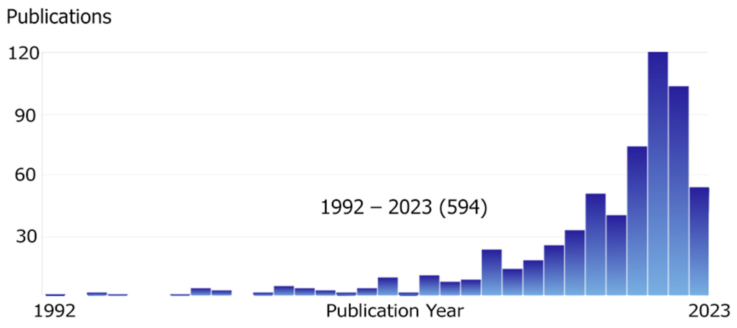
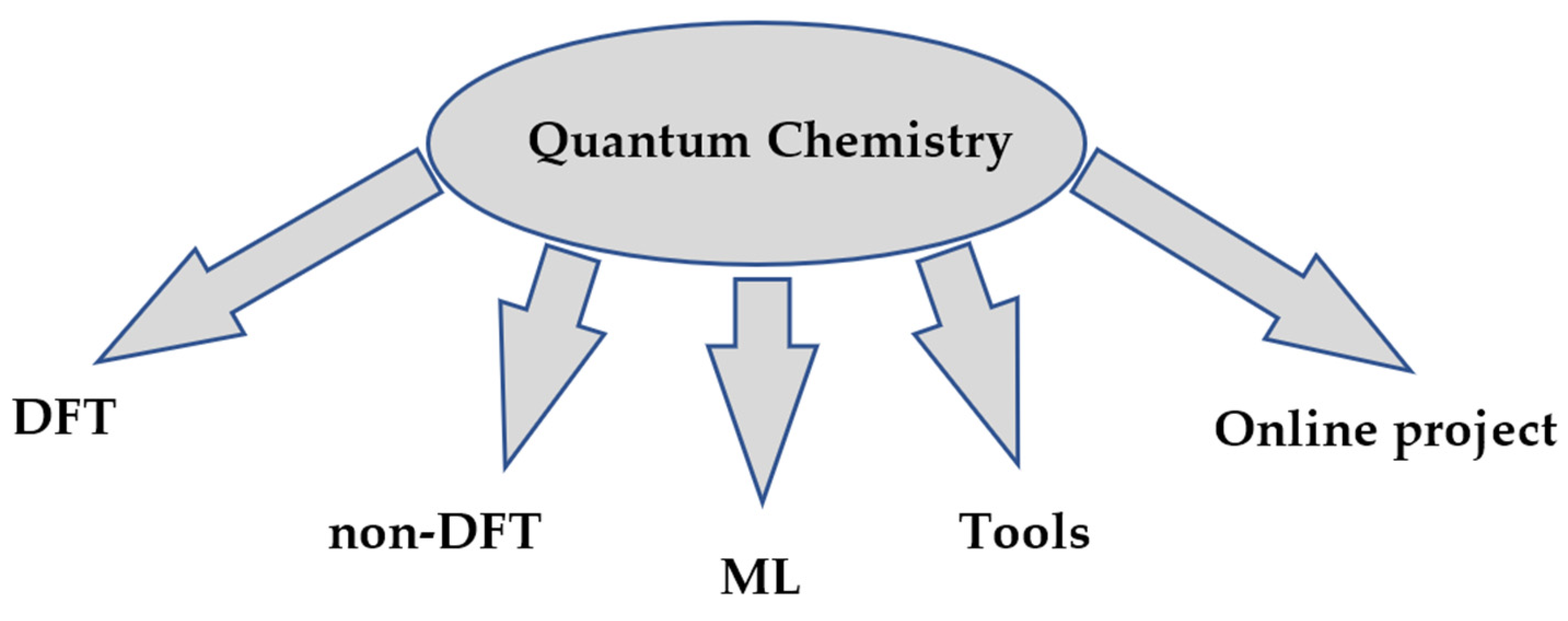
Table 1.
Python programs for the kinetics.
| Library | Kinetic Theory | Tunnel Effect | Phase | Molecularity |
|---|---|---|---|---|
| Transitivity [13] | TST CKT 1 | d-TST | Gas Solution, Surface reactions, Enzyme-catalyzed reactions | Uni/bi |
| Eyringpy [14] | TST MT CKT | Wigner Eckart | Gas Solution | Uni/bi |
| Micki [15] | TST | Wigner | Gas | Uni/bi |
| RMG [16,17,18] (Arkane) | TST (RRKM) CKT | Wigner Eckart | Gas Solution | Uni/bi |
| TAMkin [19] | TST (RRKM), VTST | Wigner Eckart | Gas | Uni/bi |
| TUMME [20] | TST (RRKM), VTST | Wigner Eckart | Gas Surface reactions on catalyst | Uni/bi |
| Pilgrim [21] | VTST, SCT | SCT | Gas Solution Condensed phases | Uni/bi |
| Polymatter [22] | TST, VTST, other | – | Gas Plasma | Uni/bi |
| Vulcan [23] | TST (RRKM), VTST | Small-curvature tunneling | Exoplanetary reactions | Uni/bi |
| RPMDrate [24] | Polymer molecular Dynamics | RPMDrate | Gas | Uni/bi |
| MORESIM [25] | REMD(H-RE, resRE) | – | Gas | Uni/bi |
| CKBIT [26] | – | – | Gas Solution Solid | Uni/bi |
| pyJac [27] | – | – | Gas Solution | Uni/bi |
| SIR model [28] | Virus spread analog | – | – | – |
1 CKT—Collins–Kimbal Theory. VTST—Variational Transition State Theory; d-TST—deformed-TST; RMG –Reaction mechanism generator (Arkane package); RRKM—Rice-Ramsperger-Kassel-Marcus theory; Uni—unimolecular reactions; bi—bimolecular reactions; REMD—Replica Exchange Molecular Dynamics; H-RE—Hamiltonian Replica Exchange; resRE—Reservoir Replica.
Table 2.
Python programs for thermodynamics.
| Library | Approach | DFT | Phase | Scope |
|---|---|---|---|---|
| pMuTT [30] | Statistical mechanics | GROMACS, Gaussian, Cantera | Gases, liquids, solids | Systems/ Reactions/Components |
| Pasta [31] | Statistical mechanics (pMuTT) | Quantum Espresso, SIESTA, VASP | – | Transition states |
| ASE 1 [32] | Statistical mechanics | ABINIT, CASTEP, CP2K, FHI-aims, Gaussian, GPAW, NWChem, Octopus, Quantum Espresso, VASP | Gases, liquids, solids | Systems/ Reactions/Components |
| TAMkin [19] | Statistical mechanics based on NMA (MBH, PHVA, MC) | Gaussian, Q-Chem | Gas | Systems/ Reactions/Components |
| AFLOW-CCE [33] | Statistical mechanics based on CCE (NMA—quasiharmonic Debye model) | VASP (LDA, PBE, SCAN), QUANTUM ESPRESSO, AIMS, ABINIT, ELK, CIF, | Ionic liquids or solids | Systems/ Reactions/Components |
| Pymatgen [34] | Internal library | VASP, ABINIT, Gaussian | – | Systems/ Reactions/Components |
| OC2020 [35] 2 | Machine learning model/Dataset | VASP, RPBE, Bader/LOBSTER | Solids | Systems |
| RMG [16,17,18] | Machine learning model (parameters dataset) | – | Gas, Solution | Components |
| pGrAdd [36] | Dataset of group additivity | – | Gas | Systems/ Reactions/Components |
| PYroMat [37] | Models Dataset | – | Gas, liquids | Components/Systems |
| ETM [38] | UNIFAC, SRK | – | Gas-liquid | Systems |
| IFG [39] | Fermi–Dirac statistics | – | Gas | Systems/Components |
| The First Law [40] | The First law of thermodynamics | – | Gas | Systems |
1 ASE—The atomic simulation environment—A Python library for working with atoms; 2 OC2020—The Open Catalyst 2020 (OC20) dataset; NMA—Normal mode analysis; MC—Monte Carlo; MBH—Mobile Block Hessian; PHVA—Partial Hessian Vibrational; IFG—Thermodynamic coefficients of ideal Fermi gas; CCE—coordination corrected enthalpies; LDA—Local Density Approximation, PBE—Perdew-Burke-Ernzerhof; SCAN—Strongly Constrained and Appropriately Normed; VASP—Vienna ab initio simulation package; UNIFAC—universal functional activity coefficient; SRK—Soave-Redlich-Kwong; ETM—Enhanced thermodynamic modeling for hydrothermal liquefaction.
Disclaimer/Publisher’s Note: The statements, opinions and data contained in all publications are solely those of the individual author(s) and contributor(s) and not of MDPI and/or the editor(s). MDPI and/or the editor(s) disclaim responsibility for any injury to people or property resulting from any ideas, methods, instructions or products referred to in the content. |
© 2023 by the authors. Licensee MDPI, Basel, Switzerland. This article is an open access article distributed under the terms and conditions of the Creative Commons Attribution (CC BY) license (https://creativecommons.org/licenses/by/4.0/).
Share and Cite
MDPI and ACS Style
Ryzhkov, F.V.; Ryzhkova, Y.E.; Elinson, M.N. Python in Chemistry: Physicochemical Tools. Processes 2023, 11, 2897. https://doi.org/10.3390/pr11102897
AMA Style
Ryzhkov FV, Ryzhkova YE, Elinson MN. Python in Chemistry: Physicochemical Tools. Processes. 2023; 11(10):2897. https://doi.org/10.3390/pr11102897
Chicago/Turabian StyleRyzhkov, Fedor V., Yuliya E. Ryzhkova, and Michail N. Elinson. 2023. "Python in Chemistry: Physicochemical Tools" Processes 11, no. 10: 2897. https://doi.org/10.3390/pr11102897
Note that from the first issue of 2016, this journal uses article numbers instead of page numbers. See further details here.