
Intelligent and Small Samples Gear Fault Detection Based on Wavelet Analysis and Improved CNN
1
School of Mechanical Engineering, Hubei University of Technology, Wuhan 430068, China
2
College of Naval Architecture and Ocean, Naval University of Engineering, Wuhan 430033, China
*
Author to whom correspondence should be addressed.
Processes 2023, 11(10), 2969; https://doi.org/10.3390/pr11102969
Submission received: 7 September 2023
/
Revised: 28 September 2023
/
Accepted: 9 October 2023
/
Published: 13 October 2023
Abstract
:Traditional methods for identifying gear faults typically require a substantial number of faulty samples, which in reality are challenging to obtain. To tackle this challenge, this paper introduces a sophisticated approach for intelligent gear fault identification, utilizing discrete wavelet decomposition and an enhanced convolutional neural network (CNN) optimized for scenarios with limited sample data. Initially, the features of the sample signal are extracted and enhanced using discrete wavelet decomposition. Subsequently, the refined signal is transformed into a two-dimensional image through a Markov transition field, preparing it for improved two-dimensional CNN training. Finally, the refined network model is applied to assess the gear fault dataset, achieving a training accuracy of 97% and a classification accuracy of 88.33%. This demonstrates the method’s feasibility and effectiveness in identifying gear faults with limited sample data.
1. Introduction
With advancements in manufacturing capabilities, mechanical equipment has evolved to become more intricate. Gears, serving as essential elements in transmitting motion and power, are ubiquitous in mechanical configurations. The prevalence of gear faults within these systems can, if not identified promptly, inflict extensive damage on the machinery, leading to potential safety hazards and significant property losses. Hence, the development of intelligent methodologies for gear fault detection and diagnosis that employ various advanced deep-learning algorithms without necessitating equipment disassembly is of paramount importance for the health management of mechanical systems [1,2].
Contemporary applications of wavelet analysis and image diagnostic methods have demonstrated remarkable accuracy in classifying gear faults, highlighting their significance in the field of intelligent gear fault identification [3]. The image diagnostic method, which is a crucial technique, enables the identification and classification of faults through deep learning [4]. Several scholars have made significant contributions to research in this field. For example, Jin et al. proposed a novel fault diagnosis method based on image recognition. This method involves processing the vibration signals of gears using wavelet packet bispectrum analysis (WPBA) to obtain bicoherence textures and extracting features from them. Finally, support vector machine (SVM) is employed to identify gear faults and their locations, achieving precise detection of gear faults in fiber manufacturing lines [5]. Li et al. collected normal vibration signals and faulty vibration signals from wind power transmission gearboxes, extracted image features from the processed data, and utilized an enhanced artificial immune algorithm for fault recognition, resulting in a 5% increase in fault recognition accuracy [6]. Additionally, Tang et al. designed a dual-channel CNN method based on compressed sensing (CS), utilizing non-contact measurements of thermal imagery and acoustic signals from mobile devices. This approach ensures precise and intelligent diagnosis of common gearbox faults, significantly improving the diagnostic accuracy of industrial helical gearboxes [7]. Liang et al. proposed a rolling bearing fault diagnosis method based on ICEEMDAN, utilizing the Hilbert transform to convert IMF components from one-dimensional time–domain signals into two-dimensional time–frequency–domain images. Subsequently, they employed a ResNet network that incorporated the attention-based attention mechanism (CBAM) structure for precise fault feature extraction. This approach yielded an accuracy rate that was 7–12% higher than that achieved with other traditional network models [8].
However, the methods aforementioned predominantly rely on conventional deep-learning methodologies, necessitating extensive fault datasets as training samples to attain optimal recognition accuracy [9]. Nonetheless, acquiring a plethora of fault data and signals is inherently challenging in real-world scenarios, and the inherent background noise complicates these data signals even further. Consequently, the practical application of deep-learning methodologies in real-world production scenarios is restricted. To counteract this limitation, researchers have introduced small-sample learning methodologies to address the diminishing accuracy of traditional deep-learning models in scenarios plagued by insufficient data availability [10]. Innovations in network structure and learning processes have been introduced to efficiently identify the networks under these circumstances. The implementation of small-sample learning methodologies mitigates the constraints induced by inadequate data availability and background noise, eventually enhancing the performance of the fault identification system. For example, Wang et al. proposed a fault diagnosis method based on the combination of a new dual-stage attention-based recurrent neural network (DA-RNN) and depth residual dispersion self-calibration convolution network (SC-ResNeSt). To address the issue of the traditional convolution layers lacking a dynamic receptive field, self-calibrated convolution modules were introduced on the basis of the distraction network (ResNeSt), and a new network model, SC-ResNeSt, was established [11]. Chen et al. proposed an adaptive multi-channel residual shrinkage network (AMC-RSN), which extracts as many features as possible by constructing an adaptive multi-channel network. They also incorporated the Meta-ACON activation function before the fully connected layer, which activates neurons based on the model’s output to achieve higher recognition accuracy under conditions of multiple faults and strong noise [12]. Su et al. introduced a data reconstruction hierarchical recursive meta-learning (DRHRML) method, illustrating significant efficacy in diagnosing small-sample bearing faults under varying operating conditions [13]. Another study by Chen et al. focused on constructing an innovative deep convolutional autoencoder neural network capable of autonomously learning different features of spectral spatial data using multiple convolutional kernels [14]. Some researchers addressed the issue of network overfitting by transferring data features or utilizing data augmentation methods to simultaneously increase the quantity of data available for network learning and reduce overfitting. Huang et al. proposed a deep multi-source transfer learning model that combines maximum mean discrepancy (MMD), local maximum mean difference (LMMD), and triplet loss for alignment. This model achieved an accuracy of over 95% in four different operating conditions of the Paderborn bearing fault dataset, making it suitable for bearing fault diagnosis under various conditions [15]. Li et al. presented a novel approach for planetary gear fault diagnosis based on intrinsic feature extraction and deep transfer learning, enabling the diagnosis of planetary gear faults [16]. Krizhevsky et al. applied random cropping of 224 × 224 patches from original images, horizontal flipping, and PCA color augmentation to enhance the data and reduce overfitting during neural network training, resulting in a 1% decrease in the model’s error rate [17].
Despite the advancements in gear fault diagnosis with limited samples, there remains a necessity for improvements in recognition accuracy and operational efficiency. To address these concerns, this study introduces an innovative small-sample learning approach for the recognition and classification of gear faults. Initially, a convolutional neural network (CNN) is utilized to exploit the two-dimensional characteristics of gear faults, aiming to attain elevated recognition rates. To augment recognition accuracy in unstable conditions, wavelet decomposition and reconstruction techniques are employed to amplify the complexity of the sample information features, thereby facilitating diverse learning within the network, enhancing its resilience, and ensuring optimal performance in intricate environments. Moreover, to rectify the dimensional incongruity between the one-dimensional vibrational signal and the two-dimensional image neural network, a Markov variation field is deployed to convert the vibrational signal into a two-dimensional image representation. To surmount the challenges posed by limited data in small-sample learning scenarios, an image enhancement technique is implemented to augment the dataset, thereby ensuring exhaustive network training. Finally, we utilize the improved convolutional neural network to conduct comparative experiments on the test dataset, achieving high recognition accuracy. This approach effectively tackles the challenges of limited sample data in real-world working conditions and the influence of background noise on recognition accuracy during actual operation. The results demonstrate that our proposed method outperforms other small-sample recognition techniques in terms of diagnostic performance, confirming its feasibility and effectiveness in gear fault detection.
2. Key Theories and Techniques
2.1. Wavelet Decomposition
Wavelet transformation rectifies the shortcomings of Fourier decomposition in analyzing non-stationary time series by replacing the sinusoidal waves of Fourier decomposition with a collection of diminishing orthogonal bases. This substitution enables the effective capture of abrupt alterations and non-stationary components within a sequence [18,19]. Gear vibration signals, which are vulnerable to noise disruption throughout the acquisition phase [20], exhibit non-stationarity and irregular variances in the time domain. Such noise disruptions can be alleviated through the meticulous decomposition and reconstruction facilitated by wavelet transformation. The discrete wavelet transform (DWT) is distinguished by non-redundant decomposition and precise reconstruction, which facilitate the separation of frequency components in gear fault vibration signals and, consequently, provide a comprehensive representation of fault characteristics [21,22]. DWT analyzes high-frequency signals and low-frequency signals using wavelet functions (high-pass filters) and scaling functions (low-pass filters). In this study, the multi-level Daubechies wavelet filter is employed, decomposing the time series signal into high-frequency detail signals through the high-pass filter and low-frequency approximation signals through the low-pass filter. To address the challenge of gear fault recognition in small-sample scenarios, we selected the Daubechies 8 wavelet bases for two compelling reasons. First, its orthogonality ensures the conservation of signal energy, which is a critical factor in the extraction of information from gear vibration signals. Second, the Daubechies 8 wavelet bases functions possess tight support in the time domain, rendering them highly suitable for scrutinizing local signal features. This characteristic proves instrumental in the detection of various gear faults based on vibration signals. By executing profound decomposition using DWT, the low-frequency signals derived from the preliminary low-pass filter decomposition can undergo further segmentation through these two filters, thus enriching the signal quantity. The DWT decomposition process is articulated as per Equation (1):
In this equation, represents the low-frequency signal at layer , denotes the high-frequency signal at layer , is the low-pass filter, and is the high-pass filter. When a signal of length N is subjected to DWT decomposition, it ultimately yields a low-frequency signal and multiple high-frequency signals. These decomposed signals have varying lengths, but their sum remains N. To harmonize the lengths of the decomposed signals with the original one, hierarchical extraction of each level’s signal is necessary succeeded by a reconstruction that matches the original signal. The reconstruction formula is as follows:
Wavelet energy elucidates the energy distribution and crucial characteristics of vibration signals across various frequency bands [23] and is suitable for classification efforts. This energy is computed by summing the squares of the decomposed signal coefficients. To understand the contribution of each decomposition level to the total energy, the wavelet energies at each level are quantified, and their proportional energy with respect to the total energy is then calculated using the following formula:
In this equation, represents the matrix of wavelet energy percentages, corresponds to the number of signals discerned post-wavelet decomposition that is equivalent to the summation of decomposition levels and one, denotes the length of each signal post-wavelet decomposition, and characterizes the matrix of signals discerned after wavelet decomposition. The percentage of wavelet energy indicates the distribution of critical features in the gear vibration signal and serves as a fundamental criterion for weight classification [24].
2.2. Markov Transition Field
The Markov transition field (MTF) acts as a mediator in signal recognition by converting the one-dimensional gear vibration signal into a two-dimensional representation to accentuate its attributes [25,26]. MTF, which is a probabilistic transition model, categorizes a time series into quantile bins, depicting states of the sequence. Every value in the sequence is assigned to its respective quantile bin. Utilizing a first-order Markov chain, transition probabilities of each value are calculated, allowing for the formulation of a Markov matrix.
In this equation, and represent the state of a value x in the time series at moments and , respectively; hence, represents the probability that a point currently in state will transition to state . Given the memoryless nature of a Markov chain, the deduced transition matrix is solely contingent on the preceding state, causing a subsequent loss of invaluable data. To mitigate this information loss, this study extends the matrix to the Markov transition field . Instead of segregating the time series into quantile bins, the dataset is segmented directly into bins along the temporal axis with bins corresponding to timestamps and being represented as and , respectively. depicts the transition probability from to , represented through the ensuing matrix:
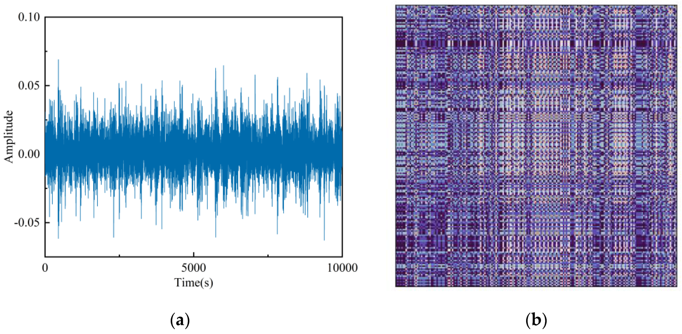
By deriving the Markov transition matrix from the time series signal, matrix elements can be employed as pixels to metamorphose the one-dimensional time series signal into a two-dimensional image using Matlab’s graphic capacities. Figure 1 showcases the bidimensional image emanated from the time series signal post-transformation via the Markov transition field.
2.3. Improved Convolution Neural Network
2.3.1. Improvement of Network Structure
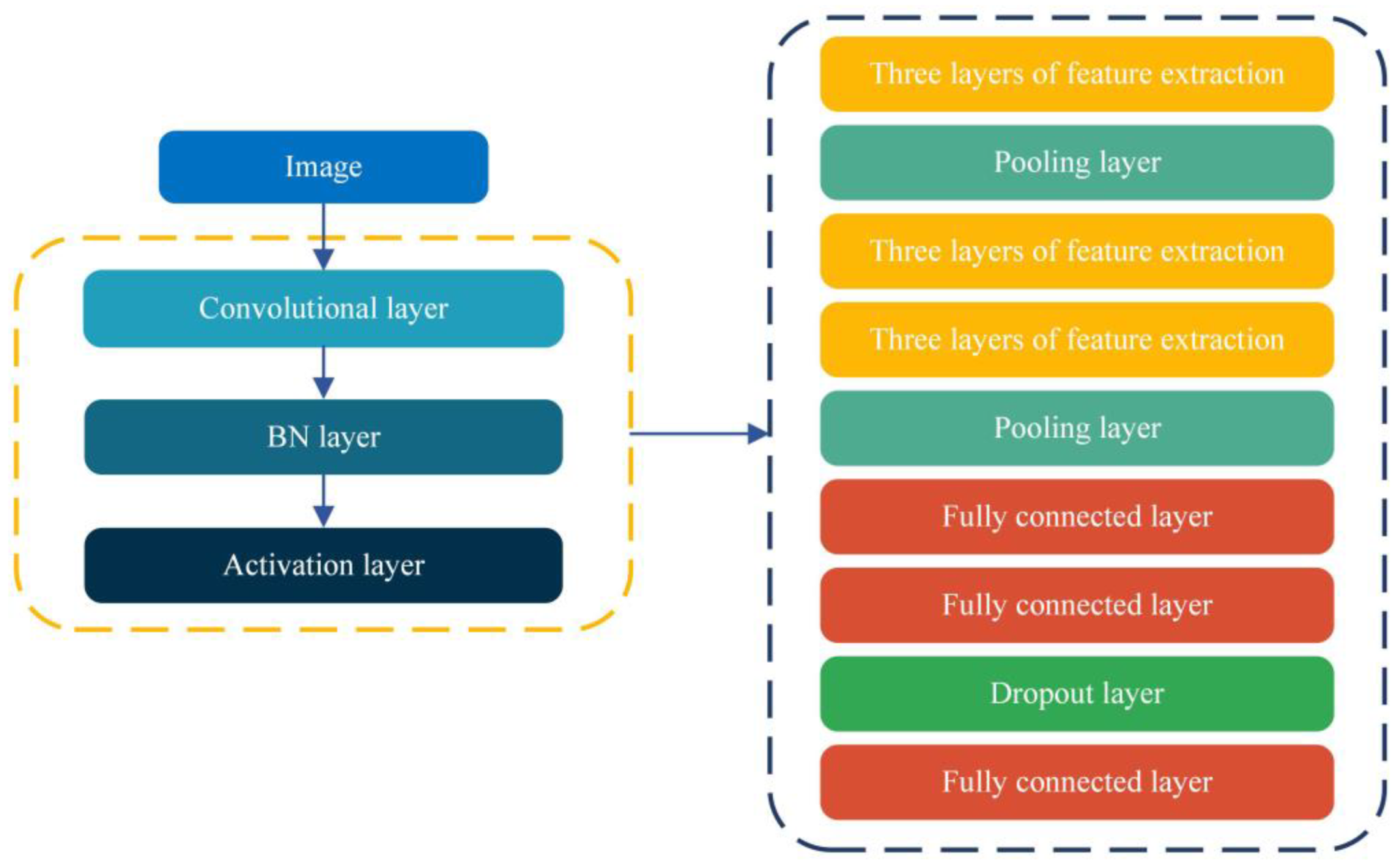
With years of advancements, the convolutional neural network (CNN) has made significant progress in the fields of image and video processing thanks to improvements in computational power [27]. This paper employs a CNN architecture that builds upon the classical VGG network structure, which includes convolutional, activation, and pooling layers. Additionally, it incorporates BN (batch normalization) layers [28] and dropout layers [29]. The customized architecture is illustrated below.
In Figure 2, each convolutional layer aggregates multiple convolutional units with every unit endowed with a convolutional kernel or filter. The calculation for each unit is delineated as follows:
In this equation, W represents the weight matrix of the convolutional kernel, symbolizes the image matrix, and stands for the bias matrix. The kernel transverses the image from left to right with a prescribed stride, computing a feature value at each interval to construe a new image or feature map drawn from the original image. During the CNN training phase, the input data distribution in each layer may oscillate due to alterations in the antecedent layer’s parameters, intensifying the complexity and resource demands for tuning hyperparameters [30]. To counteract this, a BN layer is proposed, formulated as:
In the equation, is the scaling factor that calibrates the input, while β serves as the offset factor that shifts the input accordingly. The rectified image data are then channeled through a nonlinear activation function f(x), retaining pivotal features and mitigating the computational burden of the network by nullifying inconsequential features. Herein, the activation layer employs the ReLU (rectified linear unit) function [31] expressed as:
Subsequent to the activation layer, the output undergoes further refinement through a pooling layer that filters feature data, diminishes image dimensions, and bolsters computational efficiency. This layer scans the image with a 2 × 2 pooling kernel and a stride of 2 and selects the paramount value from every quadruplet of points in the image, resulting in an image with halved dimensions.
To harness the deep-learning advantages of CNNs, multiple rounds of feature extraction are performed on the original image [32]. After passing through several layers of learning, the 2D feature maps obtained from the convolutional process are transformed into a flattened 1D matrix format using fully connected layers. To mitigate the risk of rapid parameter descent, which could lead to the loss of valuable feature information and address non-linearity issues during the learning process, this study incorporates three fully connected layers for dimensionality reduction. The fully connected layer operates in a manner similar to the convolutional layer with the distinction that the resulting data, after scanning the image, are organized in a 1D matrix format. Furthermore, to optimize the CNN, dropout layers are introduced within the fully connected layers. By randomly excluding redundant information, dropout helps mitigate overfitting and enhances the accuracy of the model.
2.3.2. Adjust Network Parameters
To facilitate deep feature learning from the small-sized original input image, this paper employs a convolutional layer configuration in which all convolutional kernels scan and traverse the output image of the previous layer with a step size of 1. Simultaneously, to enhance the extraction of edge information, the adaptive zero-padding method is utilized to ensure that the image’s dimensions (length and width) remain unchanged after each convolutional layer operation. Drawing from insights gained from previous networks with outstanding performance and considering the specific characteristics of the current gear vibration signal dataset, we have meticulously optimized and adjusted the parameters of the convolutional kernels in the four convolutional layers. These parameters are now definitively set as 5 × 5 × 16, 3 × 3 × 64, 3 × 3 × 128, and 3 × 3 × 256, respectively. Figure 3 illustrates the size changes of a grayscale image with initial dimensions of 332 × 332 after passing through a convolutional neural network.
2.3.3. Optimize Network Weights
The convolutional operations generate new images that symbolize the visual information extracted by each convolutional kernel. After their aggregation, these images are relayed to subsequent layers for advanced processing, culminating in the final, fully connected layer that ascertains the predicted class probabilities. This progression is referred to as the forward propagation of the CNN. To recalibrate the network weights across layers, backward propagation is executed that involves weight and bias adjustments. This study utilizes the cross-entropy loss function (CELF) [33] to calculate the loss value with the Adam optimizer orchestrating the network weight updates. The computation of the CELF is as follows:
In this equation, represents the total number of classes. The indicator function is assigned a value of 1 when the true class of sample aligns with ; otherwise, it takes on a value of 0. The predicted probability signifies the likelihood of sample being classified under class . Following the forward propagation of the neural network, probabilities corresponding to each class are determined. To calculate the loss value, which quantifies the deviation between the predicted probabilities and the actual labels, the cross-entropy loss function (CELF) is utilized. The Adam optimizer, which is well-known for its effectiveness, is employed to update the network weights with the aim of minimizing the loss value indicated by the CELF. The algorithm for updating via the Adam optimizer unfolds as follows:
In the equation, and represent the weight update and bias update for first-order moment estimation, respectively, and represent the weight update and bias update for first-order moment estimation, respectively, and are hyperparameters controlling the decay rate of the moving averages, and and are bias correction formulas to prevent very small gradients at the beginning of the optimization. Based on Equation (11), the gradient update algorithm for Adam can be summarized as follows:
In the equation, denotes the gradient at moment , and is the step size, generally taken to be 0.001. is a very small constant designed to prevent the denominator from being zero. In this paper, we introduce a learning rate decay strategy to optimize the network training process, which increases the gradient and reduces the experimental error by decaying the learning rate of Adam’s optimizer in equal steps.
3. Fault Diagnosis Method of Gear
3.1. Training Convolution Neural Network
To attain a proficient convolutional neural network for effective fault identification in gear vibration signals, a comprehensive training process is imperative. This training procedure involves the iterative weight updates within the network, ultimately resulting in a highly accurate model. The training process, delineated in Figure 4, encompasses five distinct stages:
- Wavelet decomposition: Initially, the original signal undergoes wavelet decomposition;
- Markov transformation: The decomposed signal is then transformed into a 2D image signal via the utilization of a Markov matrix;
- Image transformation: A plethora of new images is generated by applying various operations, such as folding and rotation, to the 2D image signals;
- Make a type label: Type labels are assigned with 70% of the data allocated for training purposes and the remaining 30% reserved for validation;
- Training convolution neural network: Labeled data are subsequently fed into the neural network, culminating in the creation of a model with heightened accuracy.
In Figure 4, the initial step involves preparing the dataset for input into the neural network. The convolutional neural network utilized in this study is a two-dimensional network; hence, the dataset must satisfy two fundamental requirements: first, the dataset should consist of two-dimensional images to align with the network’s dimensions, and second, the dataset should be sufficiently extensive to ensure thorough weight updates within the network. However, due to the nature of gear vibration signals, which are one-dimensional time series data, obtaining a large number of fault signals as training samples is challenging as they occur infrequently during normal operation. Moreover, small sample sizes contain limited feature information due to data scarcity, potentially leading to reduced performance of the highly accurate network on the test dataset. This drop in performance signifies a decline in the network’s generalization ability. Consequently, increasing the quantity of signal features is imperative.
In this study, we employ the discrete wavelet decomposition and hierarchical reconstruction method proposed in the previous section to decompose the data into low-frequency and high-frequency signals, both of which have the same length as the original signal. This approach enhances the feature information of the signals. Subsequently, we calculate the Markov transition matrices for each decomposed signal. These two-dimensional probability matrices are then converted into pixel matrices, which are subsequently output and saved as two-dimensional images. In this manner, the features of small-sample data can be represented by multiple two-dimensional images. These images are further transformed through operations such as flipping, brightness adjustment, angle rotation, and others, generating a substantial number of new images. These new images serve as the training dataset for the small-sample data, effectively achieving data augmentation. To illustrate, the transformation process for creating a training dataset that meets the requirements from a small sample consisting of 48 vibration acceleration data points is depicted in Figure 5.
Once the training dataset is prepared, it can be input into the neural network for learning. The learning process follows several steps. First, the training dataset is labeled with class categories to facilitate computer processing. For example, the four classification tasks of gear tooth breakage, chipped, health, miss, root, and surface are assigned labels 0, 1, 2, 3, and 4, respectively, with each label representing a specific signal type. Next, the entire training dataset is randomly divided into training and validation sets in a 7:3 ratio. The training set is utilized for network learning, while the validation set is used to assess the network’s performance on unseen data. This evaluation helps determine if the network has overfit and provides insights into its classification accuracy. The learning process concludes when the network reaches a sufficient number of learning iterations and maintains high accuracy on the validation set. At this stage, the network’s weights and architecture are saved, marking the end of the training process.
3.2. Weight Allocation Mechanism Based on Wavelet Energy Ratio
Although the network undergoes validation using the validation set during training, this validation method only involves label classification on the validation set. For instance, in the case of the dataset created from a single sample, as depicted in Figure 5, applying the aforementioned classification method to classify 1000 images does not consistently lead to the correct classification of that sample. If we aim to obtain the correct classification result for that sample, one possible approach is to consider using the mode, which involves selecting the most frequent label as the predicted label. However, considering the presence of interference in real-world signal scenarios and the fact that this issue can be amplified during small sample learning, it is necessary to have an appropriate weight allocation mechanism to address this problem even after achieving a high-accuracy network.
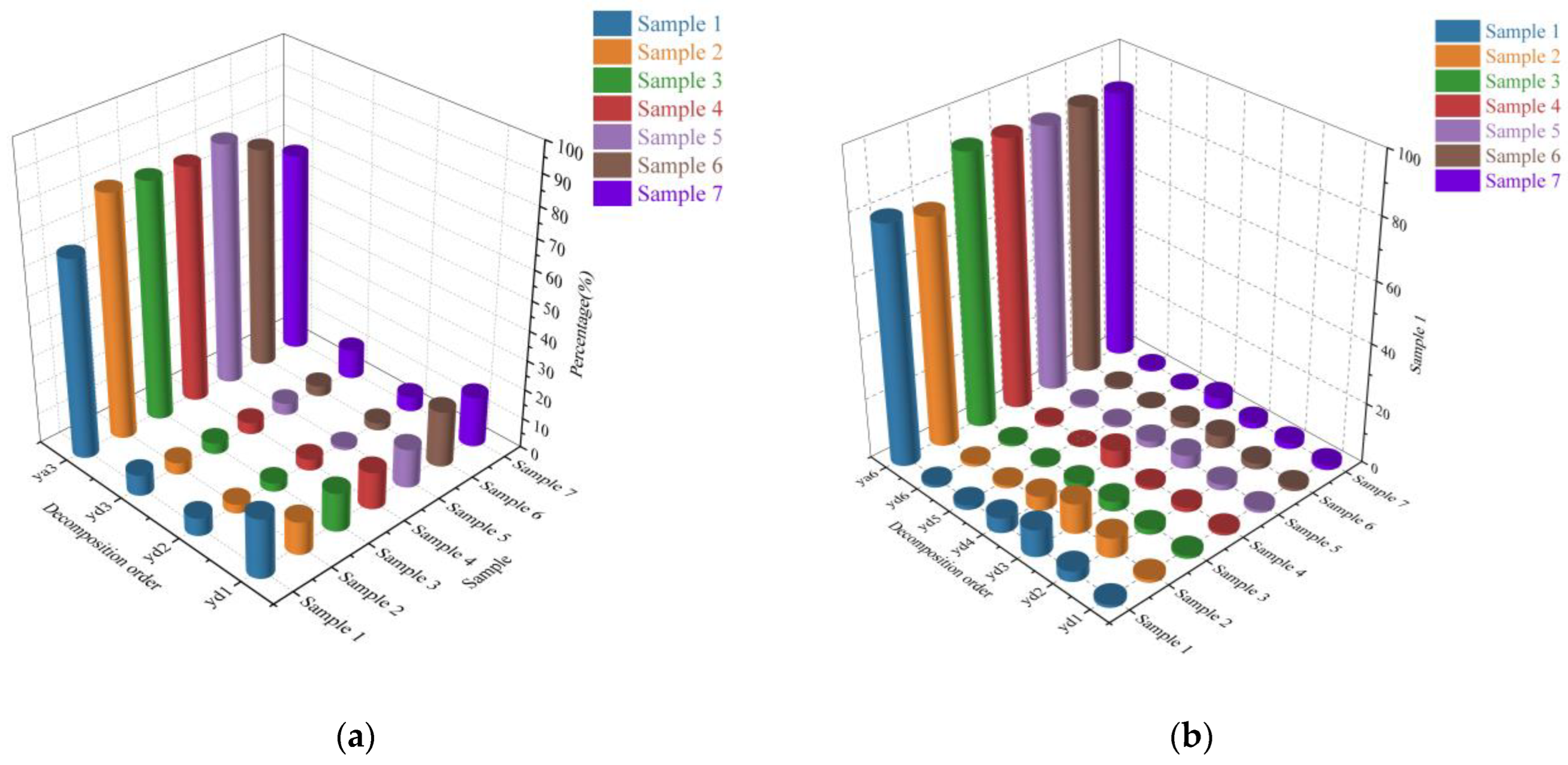
This study employs discrete wavelet decomposition to break down the signal into high-frequency and low-frequency components. Noise interference in gear vibration signals typically concentrates in the high-frequency component denoted as ‘yd’. Consequently, it is possible to assign a higher weight to the decomposed low-frequency signal and a lower weight to the high-frequency signal. This approach helps mitigate the impact of noise interference on classification accuracy. Given that the wavelet energy of gear vibration signals primarily resides in the low-frequency component denoted as ‘ya’ and is relatively less prominent in the high-frequency component (as illustrated in Figure 6), this paper utilizes this characteristic of wavelet energy to allocate weights to the classification labels. The weight allocation algorithm is as follows:
In this equation, represents the matrix of wavelet energy ratios, represents the matrix of classification labels, and represents the predicted labels for the samples.
As portrayed in Figure 7, to maintain network coherence, the classification progression for the test dataset encompasses several phases. Initially, the test dataset undergoes analogous preprocessing as the training dataset, incorporating wavelet decomposition and Markov transformation and foregoing the necessitation for image transformation and label creation operations. Subsequently, the transformed image dataset, derived from the Markov transformation, is directly integrated into a CNN, yielding individual image labels. Next, the decomposed wavelet energy is calculated to serve as weights, which are then assigned to the neural network’s predicted labels utilizing Equation (12), facilitating the formulation of weighted predicted labels. Eventually, these labels are correlated to signal categories, adhering to the label-to-class relation, which concludes the classification procedure for the test dataset.
4. Experimental Process and Analysis
4.1. Prepare Experimental Data
Utilizing the publicly accessible gearbox dataset from Southeast University in China, we created a small sample dataset for analysis that encompassed five distinct gear health conditions: chipped, healthy, missing, root, and surface. For each data category, we randomly selected a sequence of 48 consecutive data points to form a data file, resulting in the small-sample dataset presented in Table 1. The dataset comprises two primary data clusters. The first cluster consists of five files, each representing conditions such as missing teeth, incised roots, cracks, wear, and health. Each file contains 48 data points and serves as the training dataset for the network. Conversely, the second data cluster comprises 240 files with 48 files dedicated to each of the five conditions. Each file contains 48 data points and is used as a test dataset for evaluation purposes.
Table 2 displays selected data points from the training dataset, featuring the initial 12 data points for each of the five categories. The structure of the data within an individual file in the test dataset mirrors that of the training dataset except for the higher number of files in the test dataset.
4.2. Training the CNN
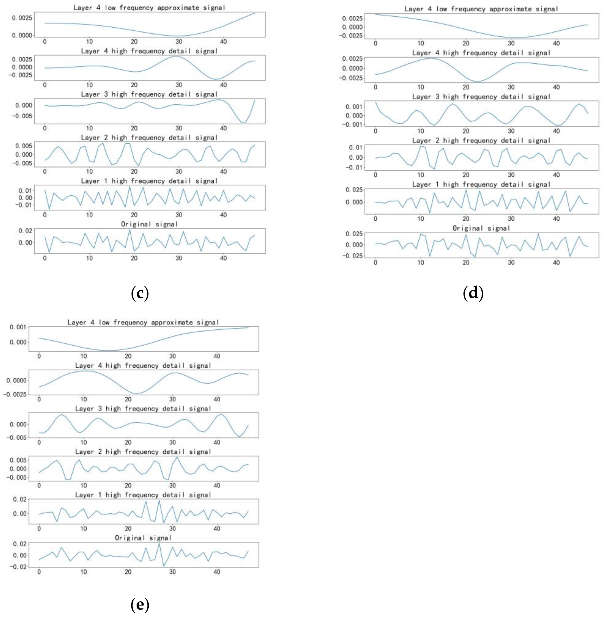
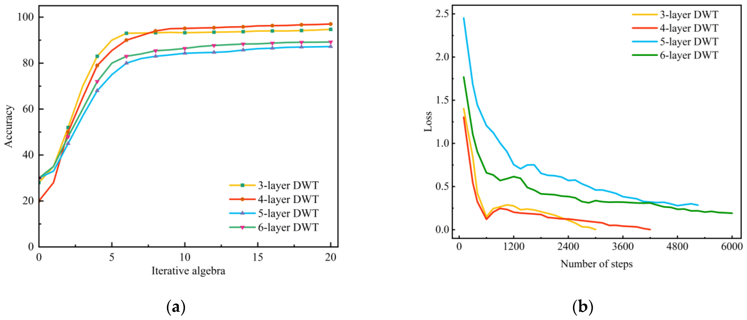
The original training dataset (as shown in Table 1) underwent training using the CNN training process depicted in Figure 4. Within the wavelet decomposition phase, we conducted decomposition at various levels (three, four, five, and six) to assess their influence on the experimental outcomes. Here, we will primarily focus on the four-layer wavelet decomposition with signal decomposition results illustrated in Figure 8. Following the four-layer wavelet decomposition, the original set of five fault signals from the training data produced 25 signals. These signals were used to calculate the Markov transition field and transform them into two-dimensional images. Subsequently, we applied data enhancement techniques, including image flipping and rotation, to augment the image dataset. This process resulted in the generation of 200 images for each signal, resulting in a total of 5000 images. Figure 9 displays some of these images used for classification. These images were labeled and randomly divided into training and validation sets at a ratio of 7:3 for input into the neural network training. The network was trained over 20 iterations with each iteration involving the processing of the entire image dataset. To expedite network learning, we configured the network to read 64 images in each cycle. The network updated weights after processing each set of 64 images. Upon processing all 5000 images, the iterative process concluded. The loss and accuracy curves obtained during training are presented in Figure 10. It is evident from the curves that the network’s loss value continually decreased throughout the training process without any significant increases, indicating the absence of overfitting. The recognition accuracy achieved following the four-layer wavelet decomposition reached 97.0%, while the accuracy levels after three-, five-, and six-layer decomposition stood at 94.7%, 87.2%, and 89.2%, respectively.
4.3. Validation of the Test Dataset
When evaluating the performance of the gear fault recognition method introduced in this study, establishing a test dataset is imperative. To guarantee the precision and effectiveness of the evaluation results, it is crucial to include an ample number of data points in the test dataset. In this research, we generated a test dataset comprising 2304 data points. More precisely, we created 48 data files for each fault type with each data file containing 48 test data points.
The test dataset underwent the process illustrated in Figure 7. Initially, it underwent wavelet decomposition with subsequent computation of wavelet energy and Markov transition fields for all decomposed signals. These Markov transition fields were then converted into a set of two-dimensional images. These images were fed into the pre-trained neural network, which assigned sample labels to each image. These labels were later used in the wavelet energy calculation formula (Equation (12)), resulting in category labels for the test dataset. By applying the mapping relationship between category labels and categories (as presented in Table 3), the fault prediction category for each data file was determined. Finally, the predicted categories were compared to the actual categories, as depicted in Figure 11, leading to the classification results displayed in Table 4.
4.4. Comparative Experiments
To further underscore the effectiveness of the method proposed in this study, we conducted two sets of comparative experiments. First, we performed comparative experiments on the small-sample detection method using datasets of various sizes. Specifically, we utilized four sets of samples, each containing 40, 32, 24, and 16 data points, and the corresponding accuracy results are depicted in Figure 12. Second, we compared the accuracy of the method proposed in this study with three other important fault detection algorithms: DBN, SVM, and ANN. The accuracy of these four detection methods on the test dataset created for this study is presented in Table 5.
Based on the classification accuracy of sample data of different sizes presented in Figure 12 and the performance of the four different detection methods on the test dataset as shown in Table 5, we can draw the following conclusions. The algorithm proposed in this study achieves a classification accuracy of over 80% when the sample data size is greater than 32 data points, but it exhibits lower accuracy and poorer detection performance when the data size is below 24 data points. Using the DBN and SVM detection methods for classifying the test dataset results in classification accuracies above 80%, but their performance is inferior to the recognition method proposed in this paper. When employing ANN for classifying the test dataset, the classification accuracy is only 60.27%, indicating lower diagnostic effectiveness.
We trained the convolutional neural network for fault classification using an Intel i5-12500H processor paired with an NVIDIA GeForce RTX 3050 4GB GPU configuration. During training, the CPU utilization was at 70%, while the GPU utilization was at 10%.
4.5. Analysis of Experimental Results
Within the experimental process, we initially used the prototype training set to train the refined 2D convolutional neural network. We continually optimized the network parameters to achieve higher accuracy. Subsequently, we applied the test dataset to simulate gear faults, which were then classified using the trained network model. Since the original training set included only one data file for each fault type, containing just 48 data points, and had a limited sample size, data augmentation was essential. After wavelet decomposition and conversion into 2D images, we still achieved improved training accuracy. To obtain more precise recognition accuracy, we created an extensive testing dataset for this investigation. We generated 48 data files for each fault type, each consisting of 48 data points, which resulted in a total of 2304 data points. Upon evaluating the testing dataset, we confirmed that the network trained using the proposed methodology demonstrates superior generalization capabilities. It maintains optimal identification efficacy even when recognizing a substantial volume of fault data with the cumulative accuracy exceeding 85%.
During the network model’s validation utilizing the test dataset, an exploration into the influence of various wavelet decomposition levels on classification accuracy was undertaken. The revelations in Table 4 insinuate that the interrelationship between the network’s recognition accuracy with differing wavelet decomposition levels and the accurate classification of the test set is not inherently linear. This is attributed to the indispensable weight allocation throughout the classification phase, which is modulated by the energy stemming from the wavelet decomposition and the noise inherent in the acquired signals. When cultivating the network model employing the original training set, the ramifications of distinct wavelet decomposition levels on training accuracy were scrutinized. Figure 10a illustrates that the network’s accuracy does not ascend proportionally with the intensification of decomposition levels. Intriguingly, the network attains paramount accuracy with a quartet of wavelet decomposition levels. This phenomenon can be ascribed to the heightened complexity introduced to the signal features by superior decomposition levels, potentially causing the network to over-simplify the learning trajectory and neglect pivotal features and, thereby, diminishing recognition accuracy.
5. Conclusions
This research introduces a novel methodology for the intelligent identification of gear faults through an enhanced convolutional neural network under conditions of insufficient sample data. Initially, the method employs discrete wavelet decomposition to expand the small-sample signal data and enriches the convolutional neural network structure by incorporating BN (batch normalization) and dropout layers to bolster the network’s generalization ability. Subsequently, a Markov transition field is invoked to metamorphose the signals derived from wavelet decomposition into two-dimensional images, thereby rendering them amenable to neural network utilization. To counteract the limitations posed by scarce data in small-sample settings, additional data augmentation is realized through image transformation methods. Preceding the application of the network model, a wavelet energy ratio-based weight allocation mechanism is introduced. This technique computes the weighted sum of the energy ratios of each signal throughout wavelet decomposition juxtaposed with the predicted labels garnered from the neural network, thus proficiently mitigating noise intrusion in small-sample signals. Validation of the proposed methodology was conducted using a publicly accessible gear fault dataset with the convolutional neural network attaining a training accuracy of up to 97% and a classification accuracy of up to 88.33% on the test dataset. These findings substantiate that the convolutional neural network, when trained via this methodology, showcases exemplary accuracy, superior generalization capability, and robust resilience.
Moreover, this research delves into the repercussions of varying wavelet decomposition levels on the convolutional neural network. It unveils a nonlinear correlation between the decomposition levels and both the training accuracy of the network and the gear fault classification accuracy. Diverse decomposition levels exhibit commendable proficiency in the classification of gear fault signals. Furthermore, the gear fault detection method presented in this research offers a distinct advantage by operating efficiently with a smaller sample dataset, resulting in accelerated network recognition speed. In our experiments, the classification of the 2304 data points in the test dataset required 20 s, primarily limited by equipment performance. With enhanced equipment capabilities, the classification speed can be further improved. This feature renders the algorithm highly suitable for online gear fault type detection. Nonetheless, the proposed methodology does warrant enhancements. More pointedly, the identification of a more efficacious weight allocation mechanism for the gear fault dataset is imperative to augment the method’s discriminative prowess on unrecognized datasets, thereby demarcating the ensuing avenue of investigation for this manuscript.
Author Contributions
Conceptualization, J.H. and T.S.; methodology, P.H. and C.Z.; software, P.H. and J.H.; validation, P.H. and T.S.; formal analysis, P.H.; investigation, J.H.; resources, C.Z. and T.S.; data curation, P.H.; writing—original draft preparation, J.H.; writing—review and editing, P.H.; visualization, P.H.; supervision, C.Z. and T.S.; project administration, C.Z. and T.S.; funding acquisition, C.Z. All authors have read and agreed to the published version of the manuscript.
Funding
This study is supported by the National Natural Science Foundation of China (No. 51805152).
Data Availability Statement
The data involved in this article have been presented in the article.
Conflicts of Interest
The authors declare that they have no conflict of interest.
References
- Wu, Z.H.; Yan, H.; Zhan, X.B.; Wen, L.; Jia, X.S. Gearbox Fault Diagnosis Based on Optimized Stacked Denoising Auto Encoder and Kernel Extreme Learning Machine. Processes 2023, 11, 1936. [Google Scholar] [CrossRef]
- Lin, M.C.; Han, P.Y.; Fan, Y.H.; Li, C.H.G. Development of Compound Fault Diagnosis System for Gearbox Based on Convolutional Neural Network. Sensors 2020, 20, 6169. [Google Scholar] [CrossRef]
- He, H.T.; Zhao, S.F.; Guo, W.; Wang, Y.; Xing, Z.Z.; Wang, P.F. Multi-fault recognition of gear based on wavelet image fusion and deep neural network. AIP Adv. 2021, 11, 125025. [Google Scholar] [CrossRef]
- Li, Y.; Cheng, G.; Pang, Y.S.; Kuai, M. Planetary Gear Fault Diagnosis via Feature Image Extraction Based on Multi Central Frequencies and Vibration Signal Frequency Spectrum. Sensors 2018, 18, 1735. [Google Scholar] [CrossRef]
- Jin, S.F.; Fan, D.; Malekian, R.; Duan, Z.H.; Li, Z.X. An image recognition method for gear fault diagnosis in the manufacturing line of short filament fibres. Insight 2018, 60, 270–275. [Google Scholar] [CrossRef]
- Li, L.S.; Wang, W.F.; Cai, A.M.; Li, H.; Zhang, L.W.; Liu, P.C. Mechanical Fault Diagnosis Technology of Wind Turbine Transmission System Based on Image Features. Mob. Inf. Syst. 2022, 2022, 5344652. [Google Scholar] [CrossRef]
- Tang, X.L.; Xu, Y.D.; Sun, X.Q.; Liu, Y.F.; Jia, Y.; Gu, F.S.; Ball, A.D. Intelligent fault diagnosis of helical gearboxes with compressive sensing based non-contact measurements. ISA Trans. 2023, 133, 559–574. [Google Scholar] [CrossRef] [PubMed]
- Liang, B.; Feng, W.W. Bearing Fault Diagnosis Based on ICEEMDAN Deep Learning Network. Processes 2023, 11, 2440. [Google Scholar] [CrossRef]
- Wang, P.; Fan, E.; Wang, P. Comparative analysis of image classification algorithms based on traditional machine learning and deep learning. Pattern Recognit. Lett. 2021, 141, 61–67. [Google Scholar] [CrossRef]
- Jia, P.P.; Wang, C.G.; Zhou, F.N.; Hu, X. Trend Feature Consistency Guided Deep Learning Method for Minor Fault Diagnosis. Entropy 2023, 25, 242. [Google Scholar] [CrossRef]
- Wang, H.T.; Guo, Y.F.; Liu, X.; Yang, J.; Zhang, X.H.; Shi, L.C. Fault Diagnosis Method for Imbalanced Data of Rotating Machinery Based on Time Domain Signal Prediction and SC-ResNeSt. IEEE Access 2023, 11, 38875–38893. [Google Scholar] [CrossRef]
- Chen, W.X.; Sun, K.C.; Li, X.X.; Xiao, Y.A.; Xiang, J.S.; Mao, H.L. Adaptive Multi-Channel Residual Shrinkage Networks for the Diagnosis of Multi-Fault Gearbox. Appl. Sci. 2023, 13, 1714. [Google Scholar] [CrossRef]
- Su, H.; Xiang, L.; Hu, A.J.; Xu, Y.G.; Yang, X. A novel method based on meta-learning for bearing fault diagnosis with small sample learning under different working conditions. Mech. Syst. Signal Proc. 2022, 169, 108765. [Google Scholar] [CrossRef]
- Chen, F.F.; Liu, L.L.; Tang, B.P.; Chen, B.J.; Xiao, W.R.; Zhang, F.J. A novel fusion approach of deep convolution neural network with auto-encoder and its application in planetary gearbox fault diagnosis. Proc. Inst. Mech. Eng. Part O-J. Risk Reliab. 2021, 235, 3–16. [Google Scholar] [CrossRef]
- Huang, M.; Yin, J.H.; Yan, S.M.; Xue, P.C. A fault diagnosis method of bearings based on deep transfer learning. Simul. Model. Pract. Theory 2023, 122, 102659. [Google Scholar] [CrossRef]
- Li, H.; Lv, Y.; Yuan, R.; Dang, Z.; Cai, Z.X.; An, B.N. Fault diagnosis of planetary gears based on intrinsic feature extraction and deep transfer learning. Meas. Sci. Technol. 2023, 34, 014009. [Google Scholar] [CrossRef]
- Krizhevsky, A.; Sutskever, I.; Hinton, G.E. ImageNet Classification with Deep Convolutional Neural Networks. Commun. ACM 2017, 60, 84–90. [Google Scholar] [CrossRef]
- Huang, S.Q.; Zheng, J.D.; Pan, H.Y.; Tong, J.Y. Order-statistic filtering Fourier decomposition and its application to rolling bearing fault diagnosis. J. Vib. Control 2022, 28, 1605–1620. [Google Scholar] [CrossRef]
- Duris, V.; Chumarov, S.G.; Mikheev, G.M.; Mikheev, K.G.; Semenov, V.I. The Orthogonal Wavelets in the Frequency Domain Used for the Images Filtering. IEEE Access 2020, 8, 211125–211134. [Google Scholar] [CrossRef]
- Cai, J.H.; Li, X.Q. Gear fault diagnosis based on time-frequency domain de-noising using the generalized S transform. J. Vib. Control 2018, 24, 3338–3347. [Google Scholar] [CrossRef]
- Ravikumar, K.N.; Madhusudana, C.K.; Kumar, H.; Gangadharan, K.V. Classification of gear faults in internal combustion (IC) engine gearbox using discrete wavelet transform features and K star algorithm. Eng. Sci. Technol. 2022, 30, 101048. [Google Scholar] [CrossRef]
- Lee, S.; Lee, T.; Kim, J.; Lee, J.; Ryu, K.; Kim, Y.; Park, J.W. A Study on the Application of Discrete Wavelet Decomposition for Fault Diagnosis on a Ship Oil Purifier. Processes 2022, 10, 1468. [Google Scholar] [CrossRef]
- Chen, C.M.; Li, J.Z.; Li, S.Z. Mechanical Fault Diagnosis Based on Relative Wavelet Energy. Agro Food Ind. Hi-Tech 2017, 28, 711–715. [Google Scholar]
- Ma, J.; Jiao, L. Fault Diagnosis of Planetary Gear Based on FRWT and 2D-CNN. Math. Probl. Eng. 2022, 2022, 4648653. [Google Scholar] [CrossRef]
- Wang, M.J.; Wang, W.J.; Zhang, X.N.; Iu, H.H.C. A New Fault Diagnosis of Rolling Bearing Based on Markov Transition Field and CNN. Entropy 2022, 24, 751. [Google Scholar] [CrossRef]
- Lei, C.L.; Xue, L.L.; Jiao, M.X.; Zhang, H.Q.; Shi, J.S. Rolling bearing fault diagnosis by Markov transition field and multi-dimension convolutional neural network. Meas. Sci. Technol. 2022, 33, 114009. [Google Scholar] [CrossRef]
- Li, Y.B.; Gu, J.X.; Zhen, D.; Xu, M.Q.; Ball, A. An Evaluation of Gearbox Condition Monitoring Using Infrared Thermal Images Applied with Convolutional Neural Networks. Sensors 2019, 19, 2205. [Google Scholar] [CrossRef]
- Yang, Z.J.; Lei, W.; Li, L.; Li, S.M.; Guo, S.S.; Wang, S.Q. Bactran: A Hardware Batch Normalization Implementation for CNN Training Engine. IEEE Embed. Syst. Lett. 2021, 13, 29–32. [Google Scholar]
- Wang, S.H.; Chen, Y. Fruit category classification via an eight-layer convolutional neural network with parametric rectified linear unit and dropout technique. Multimed. Tools Appl. 2020, 79, 15117–15133. [Google Scholar] [CrossRef]
- Jia, L.J.; Li, W.J.; Qiao, J.F. An online adjusting RBF neural network for nonlinear system modeling. Appl. Intell. 2023, 53, 440–453. [Google Scholar] [CrossRef]
- Boob, D.; Dey, S.S.; Lan, G.H. Complexity of training ReLU neural network. Discret. Optim. 2022, 44, 100620. [Google Scholar] [CrossRef]
- Kong, F.Z. Facial expression recognition method based on deep convolutional neural network combined with improved LBP features. Pers. Ubiquitous Comput. 2019, 23, 531–539. [Google Scholar] [CrossRef]
- Li, L.; Doroslovacki, M.; Loew, M.H. Approximating the Gradient of Cross-Entropy Loss Function. IEEE Access 2020, 8, 111626–111635. [Google Scholar] [CrossRef]
Figure 1.
Transformation of a one-dimensional time series signal (a) into a two-dimensional image (b).
Figure 1.
Transformation of a one-dimensional time series signal (a) into a two-dimensional image (b).

Figure 2.
Improved convolution neural network structure.

Figure 3.
Parameter changes of image.

Figure 4.
The training process of a CNN.

Figure 5.
Data set amplification process. (a) Small sample signal; (b) Signal after wavelet decomposition and (c) Two-dimensional images after data augmentation.
Figure 5.
Data set amplification process. (a) Small sample signal; (b) Signal after wavelet decomposition and (c) Two-dimensional images after data augmentation.

Figure 6.
The distribution of wavelet energy at different levels of decomposition: (a) 3-level wavelet decomposition and (b) 6-level wavelet decomposition.
Figure 6.
The distribution of wavelet energy at different levels of decomposition: (a) 3-level wavelet decomposition and (b) 6-level wavelet decomposition.

Figure 7.
Classification process of samples to be tested.

Figure 8.
Four-layer wavelet decomposition of gear vibration signals in different states: (a) chipped, (b) health, (c) miss, (d) root, and (e) surface.
Figure 8.
Four-layer wavelet decomposition of gear vibration signals in different states: (a) chipped, (b) health, (c) miss, (d) root, and (e) surface.


Figure 9.
A portion of images used for classification.

Figure 10.
Network accuracy curves (a) and loss values (b) for different levels of decomposition.

Figure 11.
The validation process for the test dataset.

Figure 12.
Classification Accuracy of Different Sample Sizes.


Table 1.
Detailed information of a small-sample dataset.
| Dataset Type | Number of Signal Types | Number of Files | Data Points of a Single File |
|---|---|---|---|
| Training set | 5 | 1 | 48 |
| Test set | 5 | 48 | 48 |
Table 2.
Partial data from the training dataset.
| Chipped | Health | Miss | Root | Surface |
|---|---|---|---|---|
| 0.000099 | −0.006351 | 0.00932 | 0.002831 | −0.007212 |
| −0.000266 | 0.021203 | −0.016575 | 0.003266 | −0.003612 |
| −0.00581 | −0.003597 | 0.010294 | 0.0001 | 0.000646 |
| 0.005527 | 0.005256 | 0.00652 | 0.005203 | 0.00577 |
| −0.000249 | 0.018343 | −0.00011 | 0.008528 | −0.003577 |
| −0.004404 | 0.004193 | 0.001225 | 0.008875 | 0.013957 |
| 0.019515 | 0.001658 | −0.000241 | −0.009279 | 0.0024 |
| −0.014083 | 0.005246 | −0.000982 | 0.001366 | −0.010189 |
| 0.013143 | −0.006969 | −0.005016 | 0.004518 | −0.001748 |
| 0.016012 | 0.015746 | 0.015688 | −0.00917 | 0.005802 |
| −0.026476 | 0.004352 | 0.000128 | 0.024582 | 0.005599 |
| 0.023174 | −0.013174 | −0.00914 | 0.019507 | −0.008323 |
Table 3.
Mapping of Category Labels to Categories.
| Fault Categories | Category Labels |
|---|---|
| chipped | 0 |
| health | 1 |
| missing | 2 |
| root | 3 |
| surface | 4 |
Table 4.
Classification Results of the Test.
| Decomposition Level | Network Accuracy | True/Total | Total Accuracy | |||||
|---|---|---|---|---|---|---|---|---|
| Chipped | Health | Miss | Root | Surface | Total | |||
| 3 | 94.70% | 37/48 | 45/48 | 41/48 | 40/48 | 42/48 | 205/240 | 85.42% |
| 4 | 97.00% | 36/48 | 46/48 | 46/48 | 43/48 | 37/48 | 208/240 | 86.67% |
| 5 | 87.20% | 39/48 | 43/48 | 45/48 | 42/48 | 43/48 | 212/240 | 88.33% |
| 6 | 89.20% | 35/48 | 45/48 | 43/48 | 46/48 | 40/48 | 209/240 | 87.08% |
Table 5.
Classification Accuracy of Different Methods on the Test Data Set.
| Methods | Accuracy | Training Time (s) | Classification Time (s) |
|---|---|---|---|
| This method | 88.83% | 342.03 | 20.12 |
| DBN | 81.31% | 398.34 | 24.71 |
| SVM | 82.45% | 311.3 | 25.98 |
| ANN | 60.27% | 401.23 | 19.73 |
Disclaimer/Publisher’s Note: The statements, opinions and data contained in all publications are solely those of the individual author(s) and contributor(s) and not of MDPI and/or the editor(s). MDPI and/or the editor(s) disclaim responsibility for any injury to people or property resulting from any ideas, methods, instructions or products referred to in the content. |
© 2023 by the authors. Licensee MDPI, Basel, Switzerland. This article is an open access article distributed under the terms and conditions of the Creative Commons Attribution (CC BY) license (https://creativecommons.org/licenses/by/4.0/).
Share and Cite
MDPI and ACS Style
Hu, P.; Zhao, C.; Huang, J.; Song, T. Intelligent and Small Samples Gear Fault Detection Based on Wavelet Analysis and Improved CNN. Processes 2023, 11, 2969. https://doi.org/10.3390/pr11102969
AMA Style
Hu P, Zhao C, Huang J, Song T. Intelligent and Small Samples Gear Fault Detection Based on Wavelet Analysis and Improved CNN. Processes. 2023; 11(10):2969. https://doi.org/10.3390/pr11102969
Chicago/Turabian StyleHu, Pan, Cunsheng Zhao, Jicheng Huang, and Tingxin Song. 2023. "Intelligent and Small Samples Gear Fault Detection Based on Wavelet Analysis and Improved CNN" Processes 11, no. 10: 2969. https://doi.org/10.3390/pr11102969
Note that from the first issue of 2016, this journal uses article numbers instead of page numbers. See further details here.