MiAMix: Enhancing Image Classification through a Multi-Stage Augmented Mixed Sample Data Augmentation Method

Abstract

Despite substantial progress in the field of deep learning, overfitting persists as a critical challenge, and data augmentation has emerged as a particularly promising approach due to its capacity to enhance model generalization in various computer vision tasks. While various strategies have been proposed, Mixed Sample Data Augmentation (MSDA) has shown great potential for enhancing model performance and generalization. We introduce a novel mixup method called MiAMix, which stands for Multi-stage Augmented Mixup. MiAMix integrates image augmentation into the mixup framework, utilizes multiple diversified mixing methods concurrently, and improves the mixing method by randomly selecting mixing mask augmentation methods. Recent methods utilize saliency information and the MiAMix is designed for computational efficiency as well, reducing additional overhead and offering easy integration into existing training pipelines. We comprehensively evaluate MiAMix using four image benchmarks and pitting it against current state-of-the-art mixed sample data augmentation techniques to demonstrate that MiAMix improves performance without heavy computational overhead.

1. Introduction

Deep learning has revolutionized a wide range of computer vision tasks like image classification, image segmentation, and object detection [1,2]. However, despite these significant advancements, overfitting remains a challenge [3]. The data distribution shifts between the training set and test set may cause model degradation. This is also particularly exacerbated when working with limited labeled data or with corrupted data. Numerous mitigation strategies have been proposed, and among these, data augmentation has proven to be remarkably effective [4,5]. Data augmentation techniques increase the diversity of training data by applying various transformations to input images in the model training. The model can be trained with a wider slice of the underlying data distribution, which improves model generalization and robustness to unseen inputs. Of particular interest among these techniques are mixup-based methods, which create synthetic training examples through the combination of pairs of training examples and their labels [6].

Subsequent to mixup, an array of innovative strategies were developed which go beyond the simple linear weighted blending of mixup, and instead apply more intricate ways to fuse image pairs. Notable among these are CutMix and FMix methods [7,8]. The CutMix technique [7] formulates a novel approach where parts of an image are cut and pasted onto another, thereby merging the images in a region-based manner. On the other hand, FMix [8] applies a binary mask to the frequency spectrum of images for fusion, hence achieving an enhanced mixup process that can take on a wide range of mask shapes, rather than just the square mask in CutMix. These methods have been successful in preserving local spatial information while introducing more extensive variations into the training data.

While mixup-based methods have shown promising results, there remains ample room for innovation and improvement. These mixup techniques utilize little to no prior knowledge, which simplifies their integration into training pipelines and incurs only a modest increase in training costs. To further enhance performance, some methodologies have leveraged intrinsic image features to boost the impact of mixup-based methods [9]. Recently, following this approach, some methods employ the model-generated feature to guide image mixing [10]. Furthermore, some researchers have also incorporated image labels and model outputs in the training process as prior knowledge, introducing another dimension to improve these methods’ performance [11]. The utilization of these methods often introduces a considerable increase in training costs to extract the prior knowledge and construct a mixing mask dynamically. This added complexity not only impacts the speed and efficiency of the training process but can also act as a barrier to deployment in resource-constrained environments. Despite their theoretical simplicity, in practice, these methods might pose integration challenges. The necessity to adjust the existing pipeline to accommodate these techniques could complicate the training process and hinder their adoption in a broader range of applications. Given this, we are driven to ponder an important question about the evolution of mixed sample data augmentation methods: How can we fully unleash the potential of MSDA while avoiding extra computational cost and facilitating seamless integration into existing training pipelines?

Considering the RandAugment [4] and other image augmentation policies, we are actually applying multiple layers of data augmentation to the input images, and those works have shown that a multi-layered and diversified data augmentation strategy can significantly improve the generalization and performance of deep learning models. The work RandomMix [12] starts ensembling the MSDA methods by randomly choosing one from a set of methods. However, by restricting to only one mixing mask being applied, RandomMix imposes some unnecessary limitations. Firstly, the variety of mixing methods can be highly improved if multiple mask methods can be applied together. Secondly, the diversity of possible mixing shapes can be greater if we can further augment the mixing masks. Thirdly, we draw insights from AUGMIX, an innovative approach that applies different random sampled augmentations on the same input image and mixes those augmented images. With the help of customized loss function design, it achieved substantial improvements in robustness. Inspired by this, we propose to remove a limitation in conventional MSDA methods and allow a sample to mix with itself with an assigned probability. It is essential to note that during this mixing process, the input data must undergo two distinct random data augmentations.

In this paper, we propose the MiAMix: Multi-layered Augmented Mixup. MiAMix alleviates the previously mentioned restrictions. Our contributions can be summarized as follows:

• We firstly revisit the design of GMix [13], leading to an augmented form called AGMix. This novel form fully capitalizes the flexibility of the Gaussian kernel to generate a more diversified mixing output.
• A novel sampling method of the mixing ratio is designed for multiple mixing masks.
• We define a new MSDA method with multiple stages: random sample paring, mixing methods and ratios sampling, generation and augmentation of mixing masks, and finally, the mixed sample output stage. We consolidate these stages into a comprehensive framework named MiAMix and establish a search space with multiple hyper-parameters.

To assess the performance of our proposed AGmix and MiAMix method, we conducted a series of rigorous evaluations across CIFAR-10/100, and Tiny-ImageNet [14] datasets. The outcomes of these experiments substantiate that MiAMix consistently outperforms the leading mixed sample data augmentation methods, establishing a new benchmark in this realm. In addition to measuring the generalization performance, we also evaluated the robustness of our model in the presence of natural noises. The experiments demonstrated that the application of RandomMix during training considerably enhances the model’s robustness against such perturbations. Moreover, to scrutinize the effectiveness of our multi-stage design, we implemented an extensive ablation study using the ResNet18 [1] model on the Tiny-ImageNet dataset.

2. Related Works

Mixup-based data augmentation methods have played an important role in deep neural network training [15]. Mixup generates mixed samples via linear interpolation between two images and their labels [6]. The mixed input $\tilde{x}$ and label $\tilde{y}$ are generated as:

$$\tilde{x}=\lambda x_i+(1-\lambda )x_j,$$

(1)

where $x_i$, $x_j$ are raw input vectors.

$$\tilde{y}=\lambda y_i+(1-\lambda )y_j,$$

(2)

where $y_i$, $y_j$ are one-hot label encodings.

$(x_i,y_i)$ and $(x_j,y_j)$ are two examples drawn at random from our training data, and $\lambda \in [0,1]$. The $\lambda \sim \mathrm{Beta}(\alpha ,\alpha )$, for $\alpha \in (0,\infty )$. Following the development of Mixup, an assortment of techniques has been proposed that focuses on merging two images as part of the augmentation process. Among these, CutMix [7] has emerged as a particularly compelling method.

In the CutMix approach, instead of creating a linear combination of two images as Mixup does, it generates a mixing mask with a square-shaped area, and the targeted area of the image is replaced by corresponding parts from a different image. This method is considered a cutting technique due to its method of fusing two images. The cutting and replacement idea has also been used in FMix [8] and GridMix [16].

The paper [13] unified the design of different MSDA masks and proposed GMix. The Gaussian Mixup (GMix) generates mixed samples by combining two images using a Gaussian mixing mask. GMix first randomly selects a center point c in the input image. It then generates a Gaussian mask centered at c, where the mask values follow:

$$mas{k}_{gmix}=1-exp\left(-\frac{{|p-c|}^2}{2{\sigma }^2}\right)$$

(3)

where $\sigma$ is set based on the mixing ratio $\lambda$ and image size N as

$$\sigma =\sqrt{\lambda }N$$

(4)

This results in a smooth Gaussian mix of the two images, transitioning from one image to the other centered around the point c. There are numerous other outstanding works in the realm of MSDA that we cannot enumerate exhaustively. In

Table 1. Summary of Various MSDA Methods.

Method	Description
Mixup [6]	Blends two images based on a blending factor (alpha). Corresponding labels of these images are also mixed similarly.
ManifoldMix [17]	Creates virtual training examples by interpolating between data samples in the latent space of a pretrained autoencoder.
CutMix [7]	Inspired by cutout, fills a random region of an image with a patch from another image, addressing issues of information loss and region dropout.
SaliencyMix [9]	Addresses CutMix’s issue of potentially mixing non-informative patches. Selects the salient part of an image and pastes it to another image’s random/salient/non-salient region.
FMix [8]	A type of MSDA that uses random binary masks obtained by thresholding low-frequency images from the Fourier space.
GridMix [16]	Introduces the concept of local context mapping by predicting patch-level labels. Employs local data augmentation through grid-based mixing.
Gmix [13]	Employs a Gaussian mixing mask for data augmentation.
AugMix [18]	Aims to reduce the training-test data distribution gap. Applies multiple random augmentations to an input image and merges the resultant images.
AutoMix [11]	Reformulates the mixup classification into two sub-tasks with sub-networks and a bi-level optimization framework. Uses a Mix Block to generate mixed samples under the supervision of mixed labels. Trained end-to-end with a momentum pipeline.

, we have summarized some of the most representative MSDA methods and those that will be related to our subsequent experiments.

3. Methods

3.1. GMix and Our AGMix

To further enhance the mixing capabilities of our method, we extend the Gaussian kernel matrix used in GMix to a new kernel matrix with randomized covariance. The motivation behind this extension is to allow for more diversified output mixing shapes in the mix mask. Specifically, we replace the identity kernel matrix with a randomized kernel matrix as follows:

$$\Sigma =\left[\begin{array}{cc}1& q\\ q& 1\end{array}\right]q\sim \mathcal{U}(-1,1)$$

Here, $\mathrm{\Sigma }$ is the Gaussian kernel covariance matrix. We keep the value in the diagonal as 1, which means that we do not randomize the intensity of the mixing, which should be solely controlled by the mixing ratio coefficient $\lambda$. To preserve the assigned mixing ratio $\lambda$ and to constrain the shape of the mask region, we sample the parameter q from a uniform distribution in a restricted range $(-1,1)$. By randomizing the off-diagonal covariance q, we allow the mixing mask to have a broader range of shapes and mixing patterns. To add further variation to the mixing shape, we apply sinusoidal rotations to the mixing mask by defining a rotation matrix R as follows:

$$R=\left(\begin{array}{cc}cos\theta & -sin\theta \\ sin\theta & cos\theta \end{array}\right),$$

(5)

where $\theta$ is a random rotation angle. We then rotate the mixing mask M using the rotation matrix R to obtain a rotated mixing mask $M_{rot}$ as follows:

$$M_{rot}=RM{R}^T.$$

(6)

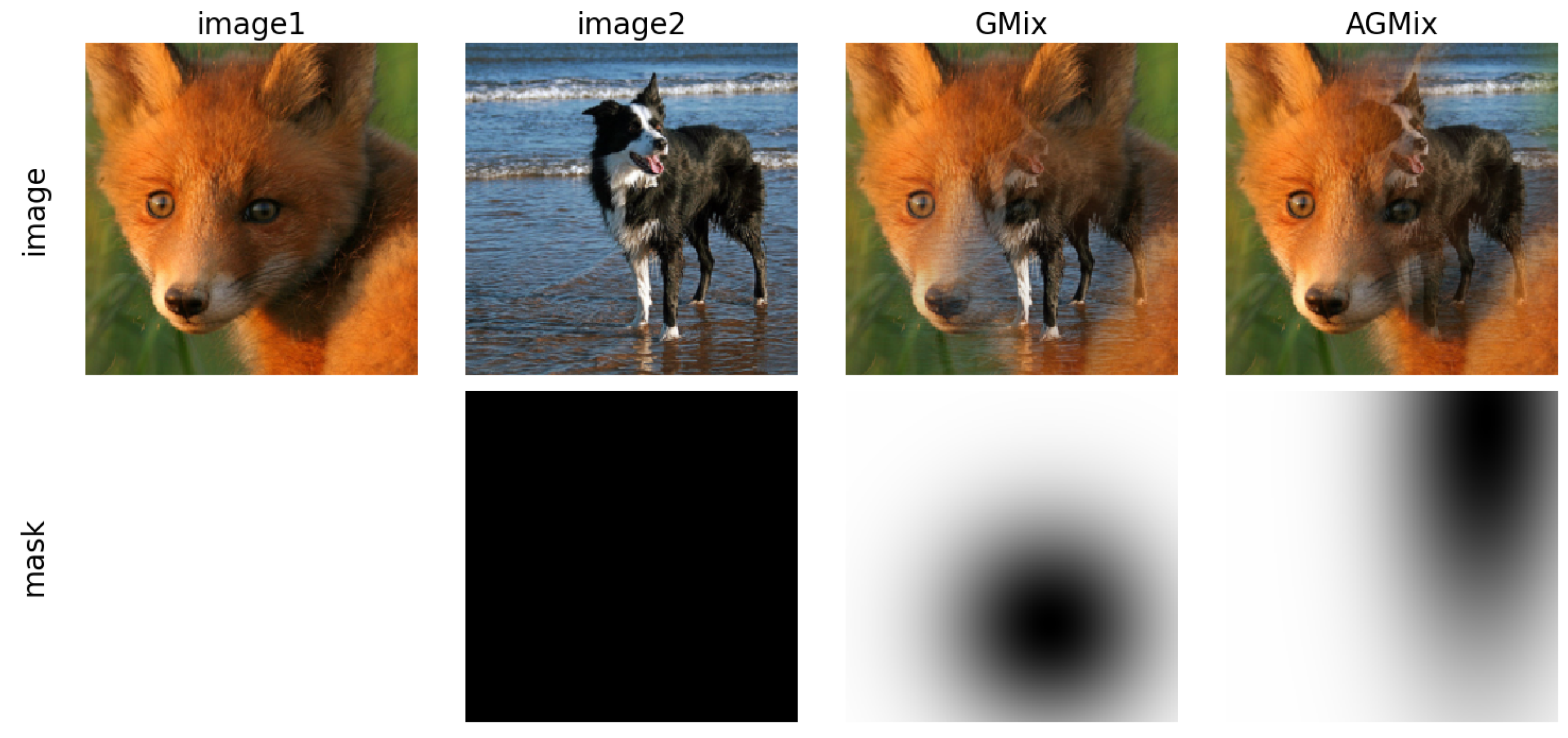
A comparative visualization between GMix and AGMix is depicted in Figure 1. This comparison underlines the successful augmentation of the original GMix approach by AGMix, introducing a wealth of varied shapes and distortions. This innovation also inspires us to apply similar rotational and shear augmentations to other applicable mixing masks. In the forthcoming experiment results section, a series of experiments provides an in-depth comparison of AGMix and GMix, further underscoring the enhancements and improvements brought by the method.

3.2. MiAMix

We introduce the MiAMix method and its detailed designs in this section. The framework is constructed by four distinct stages: random sample paring, sampling of mixing methods and ratios, the generation and augmentation of mixing masks, and finally, the mixed sample output stage. Each stage will be discussed in the ensuing subsections. These stages are presented step-by-step in Algorithm 1, the parameters are listed in Table 2, a practical illustration of the processes within each stage can be found in Figure 2, and additional examples can be found in the Appendix A.

To understand the effects of the various design choices of this proposed algorithm in this section, we conduct a series of ablation studies in the following experiment result section. We also compare our method with previous MSDA methods to justify that the MiAMix works as a balance between performance and computational overhead.

Algorithm 1: Multi-stage Augmented Mixup (MiAMix)

1: Inputs: Data samples $x_1,x_2,...,x_n$, corresponding labels $y_1,y_2,...,y_n$, 2: Parameters: mixing parameter $\alpha$, maximum number of mixing layers $k_{max}$, mixing method candidates M and corresponding sampling weights W, more parameters are listed in the Table 2 3: Outputs: Mixed samples ${\tilde{x}}_1,{\tilde{x}}_2,...,{\tilde{x}}_n$, mixed labels ${\tilde{y}}_1,{\tilde{y}}_2,...,{\tilde{y}}_n$ 4:   5: for $i=1$ to n do 6:     Sample a mixing data point $(x_t,y_t)$ either by sampling from the entire pool of data samples or alternatively, selecting itself as the mixing data point with a ratio $p_{self}$. 7:     Sample number of mixing layers k from 1 to $k_{max}$ 8:     Sample ${\lambda }_1,{\lambda }_2,\dots ,{\lambda }_k$ from a Dirichlet distribution $\mathrm{Dir}\left(\mathbf{\alpha }\right)$, where the parameter vector $\mathbf{\alpha }=({\alpha }_1,\dots ,{\alpha }_k,{\alpha }_{k+1})$, such that ${\alpha }_1={\alpha }_k=\alpha$ and ${\alpha }_{k+1}=k·\alpha$. 9:      Sample k mixing methods $m_1$, $m_2$,..., $m_k$ from M with weighted distribution over W 10:     Generate all $mas{k}_j$ from $m_j\left({\lambda }_j\right)$ 11:     Apply mask augmentation to masks 12:     Merge all the k masks to $mas{k}_{merged}$, Get the ${\lambda }_{merged}$ from the $mas{k}_{merged}$ 13:     Apply $m_{merged}$ to the sampled input pair ${\tilde{x}}_i=mas{k}_{merged}\otimes x_i+(1-mas{k}_{merged})\otimes x_t$ 14:     Apply ${\lambda }_{merged}$ to sampled label pair ${\tilde{y}}_i=\lambda y_i+(1-\lambda )y_j$ 15:     Append mixed ${\tilde{x}}_i$ and ${\tilde{y}}_i$ to output list 16: end for 17: return Mixed samples ${\tilde{x}}_1,{\tilde{x}}_2,...,{\tilde{x}}_n$, mixed labels ${\tilde{y}}_1,{\tilde{y}}_2,...,{\tilde{y}}_n$

Table 2. MiAMix Parameters.

Notation	Value	Description
$\alpha$	2	MSDA mix ratio sampling parameter
$k_{max}$	2	Maximum number of mixing layers
M	[MixUp, CutMix, FMix, GridMix, AGMix]	Mixing method candidates
W	[2, 1, 1, 1, 1]	Mixing method sampling weights
$p_{self}$	0.10	Self-mixing ratio
$p_{aug}$	0.25	Mixing mask augmentation ratio
$p_{smooth}$	0.5	Mixing mask smoothing ratio

Table 2. MiAMix Parameters.

Notation	Value	Description
$\alpha$	2	MSDA mix ratio sampling parameter
$k_{max}$	2	Maximum number of mixing layers
M	[MixUp, CutMix, FMix, GridMix, AGMix]	Mixing method candidates
W	[2, 1, 1, 1, 1]	Mixing method sampling weights
$p_{self}$	0.10	Self-mixing ratio
$p_{aug}$	0.25	Mixing mask augmentation ratio
$p_{smooth}$	0.5	Mixing mask smoothing ratio

3.2.1. Random Sample Paring

The conventional method of mix pair sampling is direct shuffling the sample indices to establish mixing pairs. There are two primary differences that arise in our approach. The first difference is that, in our image augmentation module, we prepare two sets of random augmentation results for mixing. If all images within a batch undergo the exact same augmentation, the ultimate mix’s diversity remains constrained. This observation, inspired by our examination of the open-source project OpenMixup [19], revealed a crucial oversight in prior work. In MiAMix, we addressed this issue and yielded measurable improvement. The second, and arguably more critical distinction, is the introduction of a new probability parameter, denoted as $p_{self}$, which enables images to mix with themselves and generate “corrupted” outputs. This strategy draws from the notable enhancement in robustness exhibited by AUGMIX [18]. Integrating the scenario of an image mixing with itself can significantly benefit the model, and we delve into an experimental section of this paper.

3.2.2. Sampling Number of Mixing Masks, Mixing Methods, and Ratios

Previous studies such as RandAug and AutoAug have shown that ensemble usage and multi-layer stacking in image data augmentation are essential for improving a computer vision model and mitigating overfitting [4]. However, the utilization of ensembles and stacking in mixup-based methods has been underappreciated. Therefore, to enhance input data diversity with mixing, we introduce two strategies. Firstly, we perform random sampling over different methods. For each generation of a mask, a method is sampled from a mixing methods set M, with a corresponding set of sampling weights W. The M contains not only our proposed method AGMix above but also MixUp, CutMix, GridMix, and FMix. These mixup techniques blend two images with varying masks, and the main difference between those methods is how they generate these randomized mixing masks. As such, an MSDA can be conceptualized as a standardized mask generator, denoted by m. This generator takes as input a designated mixing ratio, $\lambda$, and outputs a mixing mask. This mask shares the same dimensions as the original image, with pixel values ranging from 0 to 1. The final image can be directly procured using the formula:

$$\tilde{x}=mask\otimes x_1+(1-mask)\otimes x_2$$

(7)

In this context, ⊗ denotes element-wise multiplication, the mask is the generated mixing mask, and $x_1$ and $x_2$ represent the two original images.

Secondly, we pioneered the integration of multi-layer stacking in mixup-based methods. Therefore, we need to sample another parameter to set the mixing ratio for each mask generation step. For this, the mixup’s methodology here is:

$$\lambda \sim \mathrm{Beta}(\alpha ,\alpha ),\mathrm{for}\alpha \in (0,\infty )$$

(8)

While the Beta distribution’s original design caters to bivariate instances, the Dirichlet distribution presents a multivariate generalization. It is a multivariate probability distribution parameterized by a positive reals vector $\mathbf{\alpha }$, essentially generalizing the Beta distribution. Our sampling approach is:

$${\lambda }_1,{\lambda }_2,\dots ,{\lambda }_k\sim \mathrm{Dir}\left(\mathbf{\alpha }\right),\mathrm{for}k\mathrm{masks}$$

$$\mathrm{where}\mathbf{\alpha }=({\alpha }_1,\dots ,{\alpha }_k,{\alpha }_{k+1}),\mathrm{and}{\alpha }_1={\alpha }_k=\alpha ,{\alpha }_{k+1}=k\times \alpha$$

(9)

We maintain $\alpha$ as the sole sampling parameter for simplicity. With the Dirichlet distribution’s multidimensional property, the mixing ratios derived from sampling are employed for multiple mask generators. In other words, our MiAMix approach employs the parameter ${\lambda }_i$ to determine the mixing ratio for each mask $mas{k}_i$. This parameter selection method plays a pivotal role in defining the multi-layered mixing process.

3.2.3. Mixing Mask Augmentation

Upon generation of the masks, we further execute augmentation procedures on these masks. To preserve the mixing ratio inherent to the generated masks, the selected augmentation processes should not bring substantial change to the mixing ratio of the mask, so we mainly focus on some morphological mask augmentations. Three primary methods are utilized: shear, rotation, and smoothing. The smoothing applies an average filter with varying window sizes to subtly smooth the mixing edge. It should be explicitly noted that these augmentations are particularly applicable to CutMix, FMix, and GridMix methodologies. In contrast, Mixup and AGMix neither require nor undertake the aforementioned augmentations.

3.2.4. Mixing Output

During the mask generation step, we may have multiple mixing masks. The MiAMix employs the masks to merge two images and obtains the mixed weights for labels by point-wise multiplication.

$${\mathrm{mask}}_{product}=\prod _{i=1}^n{\mathrm{mask}}_i$$

(10)

The n denotes the number of masks, and the multiplication operation is conducted in a pointwise manner. Another approach we also tried is by summing the weighted mask:

$${\mathrm{mask}}_{sum}=\mathrm{clip}\left(\sum _{i=1}^n{\mathrm{mask}}_i,0,1\right),$$

(11)

The clipping serves to confine the mixing ratio at each pixel within the [0,1] interval. It is crucial to note that the cumulative mask weights could potentially exceed 1 at specific pixels. As a consequence, we enforce a clipping operation subsequent to the summation of masks if we sum them up.

In the output stage, our approach is different from the conventional mixup method. We sum the weights of the merged mask, $mas{k}_{merged}$, to determine the final ${\lambda }_{merged}$, which defines the weights of the labels.

$${\lambda }_{merged}=\frac{1}{H\times W}\sum _{j=1}^H\sum _{k=1}^W{\mathrm{mask}}_{merge{d}_{jk}}$$

(12)

In this equation, H and W denote the height and width of the mask, respectively, j and k are the indices of the pixels within each mask. Therefore, ${\lambda }_{merged}$ represents the overall mixing intensity by averaging the mixing ratios over all the pixels in $mas{k}_{merged}$. The rationale behind this is that, if multiple masks have significant overlap between them, the final mixing ratio will deviate from the initially set ${\lambda }_{sum}=\Sigma {\lambda }_i$, regardless of whether the masks are merged via multiplication or summation. We will compare these two ways of merging the mixing mask and two ways of acquiring the weights $\lambda$ for labels in the upcoming experimental results section.

3.3. Why a Diversified MSDA Design Excels

The work [13] established that Mixup, through linear interpolation between data samples in both input x and output y, acts as implicit regularization as well. Mathematically, this can be seen as adding a regularization term to the loss function that affects the gradient and Hessian concerning x. Differentiated variants like CutMix employ varying mixing masks. The nature of the mask greatly impacts the regularization coefficients. For instance, CutMix, as a more spatially diversified mask, achieves spatially-conscious regularization, primarily because the coefficients of these masks are pixel-distance-dependent. In contrast, the conventional mixup technique imposes uniform regularization across all pixels.

Such diversity in masking potentially enhances regularization by exposing the model to an expansive range of intermediate samples. To put it illustratively, while mixup applies regularization to prompt the model to comprehend images over an extensive range and relate distant pixels, CutMix sharpens the model’s focus, urging it to capitalize on information from adjacent pixels. The optimal mask design may be contingent on various factors, such as the specific dataset in use or the particular task at hand. For example, tasks that emphasize holistic comprehension might benefit more from mixup, whereas those that prioritize discerning localized information might find CutMix more apt. Admittedly, such strategic choices might appear to be intentionally fitting a particular data distribution. Nevertheless, it is evident that increased diversity in mixing masks yields a more potent and bespoke regularization effect. Inspired by this profound understanding, we have devised an even more diversified approach and will demonstrate its superior performance in the subsequent experimental results section.

4. Results

In order to examine the benefits of MiAMix, we conduct experiments on fundamental tasks in image classification. Specifically, we chose the CIFAR-10, CIFAR-100, and Tiny-ImageNet datasets for comparison with prior work. We replicate the corresponding methods on all those datasets to demonstrate the relative improvement of employing this method over previous mixup-based methods.

4.1. Tiny-ImageNet, CIFAR-10, and CIFAR-100 Classification

For our image classification experiments, we utilize the Tiny-ImageNet [14] dataset, which consists of 200 classes with 500 training images and 50 testing images per class. Each image in this dataset has been downscaled to a resolution of $64\times 64$ pixels. We also evaluate our methods (AGMix and MiAMix) against those mixing methods on CIFAR-10 and CIFAR-100 datasets. The CIFAR-10 dataset consists of 60,000 32 × 32 pixel images distributed across 10 distinct classes, and the CIFAR-100 dataset, mirrors the structure of the CIFAR-10 but encompasses 100 distinct classes, each holding 600 images. Both datasets include 50,000 training images and 10,000 for testing.

Training is performed using the ResNet-18 and ResNeXt-50 network architecture over the course of 400 epochs, with a batch size of 100. Our optimization strategy employs Stochastic Gradient Descent (SGD) with a momentum of 0.9 and weight decay set to $5\times {10}^{-4}$. The initial learning rate is set to 0.1 and decays according to a cosine annealing schedule.

In our investigation of various mixup methods, we select a set of methods $M=[Mixup,CutMix,Fmix,GridMix,AGMix]$. Each of these methods was given a weight, represented as a vector $W=[2,1,1,1,1]$. The mixing parameter, $\alpha$, was set to 1 throughout the experiments.

As shown in

Table 3. Comparison of various MSDAs on CIFAR-10 and CIFAR 100 using ResNet-18 and ResNeXt-50 backbones, on Tiny-ImageNet using a ResNet-18 backbone. Note that AutoMix needs additional computations for learning and processing extra prior knowledge. $TrainingCost=\frac{Trainingtime}{Vanillamodeltrainingtime}$.

Methods	CIFAR10		CIFAR100		Tiny-ImageNet ResNet-18(%)	Training Cost
	ResNet-18(%)	ResNeXt-50(%)	ResNet-18(%)	ResNeXt-50(%)
Vanilla	95.07	95.81	77.73	80.24	61.68	1.00
Mixup [6]	96.35	97.19	79.34	81.55	63.86	1.00
CutMix [7]	95.93	96.63	79.58	78.52	65.53	1.00
FMix [8]	96.53	96.76	79.91	78.99	63.47	1.07
GridMix [16]	96.33	97.30	78.60	79.80	65.14	1.03
GMix [13]	96.02	96.25	78.97	78.90	64.41	1.00
SaliencyMix [9]	96.36	96.89	79.64	79.72	64.60	1.01
AutoMix [11]	97.08	97.42	81.78	83.32	67.33	1.87
AGMix	96.15	96.37	79.36	81.04	65.68	1.03
MiAMix	96.92	97.52	81.43	83.50	67.95	1.11

AutoMix represents methods with higher training costs, hence it is colored gray. Methods highlighted with a gray background, such as MiAMix, represent our proposed methods.

, we compare the performance and training cost of several MSDA methods. The training cost is measured as the ratio of the training time of the method to the training time of the vanilla training. From the results, it is clear that our proposed method, MiAMix, shows a state-of-the-art performance among those low-cost MSDA methods. The test results even surpass the AutoMix, which embeds the mixing mask generation into the training pipeline to take more advantage of injecting dynamic prior knowledge into the sample mixing. Notably, the MiAMix method only incurs an 11% increase in training cost over the vanilla model, making it a cost-effective solution for data augmentation. In contrast, the AutoMix takes approximately 70% more training costs.

4.2. Experiment on Image Transformer Model

Image transformers [20,21] have reshaped the landscape of computer vision by achieving remarkable performance across a wide range of tasks. Given their structural differences from traditional CNN architectures, it is crucial to ensure that the data augmentation methods, especially the mixed-sample ones, generalize well with them. In this section, we present an evaluation of various mixed-sample data augmentation (MSDA) methods on the CIFAR-100 dataset using the DeiT-S Image Transformer Model. The models are trained from scratch in 200 epochs, with a batch size of 100. The Adam optimizer is applied with learning rate warm-up and decay.

As shown in

Table 4. Comparison of various MSDA on CIFAR-100 using DeiT-S Image Transformer Model.

Methods	CIFAR-100 Accuracy (%)
Vanilla	65.81
Mixup [6]	69.98
CutMix [7]	74.02
FMix [8]	70.41
GridMix [16]	69.79
SaliencyMix [9]	69.78
AutoMix [11]	76.17
MiAMix	73.98

AutoMix represents methods with higher training costs, hence it is colored gray. Methods highlighted with a gray background, such as MiAMix, represent our proposed methods.

, the incorporation of MSDA methods offers substantial improvements. Among the methods listed, MiAMix stands out by achieving a Top-1 accuracy of $73.98\%$. MiAMix demonstrates its robustness and adaptability when paired with the transformer architecture. In contrast to other mixup variants, a shift in architecture tends to induce more pronounced discrepancies in performance outcomes. This is particularly impressive, considering that transformers have intricacies that are different from traditional CNNs, emphasizing MiAMix’s wide applicability and effectiveness.

4.3. Transfer Learning

Transfer learning is a prevalent technique in modern deep learning practices. In our experiments, we utilized the CUB-200 [22] dataset, which comprises 11,788 images spanning 200 bird subcategories, with a division of 5994 for training and 5794 for testing. Images are presented at a resolution of $224\times 224$.

We employed a ResNet-18, which was pre-trained on the ImageNet-1k dataset, as our initialization checkpoint. The training was conducted over 200 epochs using the SGD optimizer with a learning rate of $1\times {10}^{-3}$, momentum set to 0.9, and a batch size of 32.

From the results showcased in

Table 5. Comparison of various MSDA on CUB-200 dataset with transfer learning. All those models are initialized from a ResNet-18 model checkpoint pre-trained on ImageNet-1k.

Methods	CUB-200 Accuracy (%)
Vanilla	77.88
Mixup [6]	79.13
CutMix [7]	79.04
FMix [8]	77.82
SaliencyMix [9]	77.95
AutoMix [11]	79.87
MiAMix	79.17

AutoMix represents methods with higher training costs, hence it is colored gray. Methods highlighted with a gray background, such as MiAMix, represent our proposed methods.

, MiAMix demonstrates commendable efficacy even under conditions of limited data availability. Moreover, its performance under the transfer learning paradigm further underscores its robustness and adaptability across diverse learning scenarios.

4.4. Robustness

To assess robustness, we set up an evaluation on the CIFAR-100-C dataset, explicitly designed for corruption robustness testing and providing 19 distinct corruptions such as noise, blur, and digital corruption. Our model architecture and parameter settings used for this evaluation are consistent with those applied to the original CIFAR-100 dataset in our above experiments. According to

Table 6. Top-1 accuracy on CIFAR-100 and corrupted CIFAR-100-C based on ResNeXt-50.

Methods	Clean Acc(%)	Corrupted Acc(%)
Vanilla	80.24	51.71
Mixup [6]	81.55	58.10
CutMix [7]	78.52	49.32
AutoMix [11]	83.32	58.36
MiAMix	83.50	58.99

AutoMix represents methods with higher training costs, hence it is colored gray. Methods highlighted with a gray background, such as MiAMix, represent our proposed methods.

, our proposed MiAMix method demonstrated exemplary performance, achieving the highest accuracy. This provides compelling evidence that our multi-stage and diversified mixing approach contributes significantly to the improvement of model robustness.

4.5. Ablation Study

The MiAMix method involves multiple stages of randomization and augmentation, which introduce many parameters into the process. It is essential to clearly articulate whether each stage is necessary and how much it contributes to the final result. Furthermore, understanding the influence of each major parameter on the outcome is also crucial. To further demonstrate the effectiveness of our method, we conducted several ablation experiments on the CIFAR-10, CIFAR-100-C, and Tiny-ImageNet datasets.

4.5.1. GMix, AGMix, and Mixing Mask Augmentation

A particular comparison of interest is between the GMix and our augmented version, AGMix, in Table 3 and Table 6. The primary difference between these two methods lies in the inclusion of additional randomization in the Gaussian Kernel. The experiment results reveal that this simple yet effective augmentation strategy indeed brings about a significant improvement in the performance of the mixup method across all three datasets and one corrupted dataset, despite maintaining almost the same training cost as GMix. As the results in

Table 7. Ablation study on mixing mask augmentation with ResNet-18 on Tiny-ImageNet. The percentage after “Smoothing” and “rotation and shear” refers to the ratio of masks applied with the respective type of augmentation during training.

Augmentations	Top-1(%)	Top-5(%)
No augmentation	66.87	86.66
+Smoothing 50%	67.29	86.82
+rotation and shear 25%	67.95	87.26

illustrate, the introduction of various forms of augmentation progressively improves model performance. These experiment results underscore the importance and effectiveness of augmenting mixing masks during the training process; furthermore, they validate the approach taken in the design of our MiAMix method.

4.5.2. The Effectiveness of Multiple Mixing Layers

The data presented in

Table 8. Ablation study on multiple mixing layers with ResNet-18 on Tiny-ImageNet. The brackets indicate that the number of turns is randomly selected from the enclosed numbers with equal probability during each training step.

Number of Turns	Top-1 (%)	Top-5 (%)
1	66.16	86.49
2	67.10	86.45
3	67.10	86.42
4	67.01	86.38
$[1,2]$ *	67.95	87.25
$[1,2,3]$ *	67.86	87.16

An asterisk (*) means that we uniformly sample a number of layers from the list during the training.

demonstrates the substantial impact of multiple mixing layers on the model’s performance. As the table shows, a discernible improvement in Top-1 accuracy is observed when more layers of masks are added, emphasizing the effectiveness of this approach in enhancing the diversity and complexity of the training data. Most notably, the model’s performance is further amplified when the number of layers is not constant but rather sampled randomly from a set of values, as indicated by the bracketed entries in the table. This observation suggests that introducing variability into the number of mixing layers could potentially be an effective approach for extracting more comprehensive and robust features from the data.

However, it is important to note that there are diminishing returns as we further increase the layers of mixing. The experimental results reveal certain limitations; particularly, an overly diversified mixing mask does not always guarantee significant performance enhancements. As the number of layers continues to grow, the increase in Top-1 accuracy begins to plateau. This phenomenon might be attributed to the potential over-complexification of the data, which may inadvertently introduce noise or ambiguities detrimental to the learning process. Therefore, based on our findings, it seems prudent to adopt a balanced approach, where the optimal configuration employs a mix of one or two layers with a sampling weight of [0.5, 0.5]. This setup offers a judicious blend of diversity and clarity, ensuring the model extracts meaningful patterns without being overwhelmed by excessive variability.

4.5.3. The Effectiveness of MSDA Ensemble

In the study, the ensemble’s efficacy was tested by systematically removing individual mixup-based data augmentation methods from the ensemble and observing the impact on Top-1 accuracy. The results, as shown in

Table 9. Effectiveness experiment of MSDA ensemble, tested on Tiny-ImageNet and CIFAR-10 datasets. Each weight corresponds to a different MSDA candidate, and a weight of zero signifies the removal of the corresponding method from the ensemble.

Weights [MixUp, CutMix, FMix, GridMix, AGmix]	Top-1 Accuracy (%)
	Tiny-ImageNet	CIFAR-10
[1, 1, 1, 1, 1]	67.51	96.86
[0, 1, 1, 1, 1]	66.81 −0.70	96.42 −0.44
[1, 0, 1, 1, 1]	66.98 −0.53	96.74 −0.12
[1, 1, 0, 1, 1]	66.95 −0.58	96.65 −0.21
[1, 1, 1, 0, 1]	66.02 −0.49	96.67 −0.19
[1, 1, 1, 1, 0]	66.86 −0.65	96.53 −0.33

The colour red is used to highlight how much the performance can degrade if the corresponding changes are made to the optimal setting which is shown in the first row.

, clearly exhibit the vital contributions each method provides to the overall performance. Eliminating any single method from the ensemble led to a decrease in accuracy, underscoring the value of the diverse mixup-based data augmentation techniques employed. This demonstrates the strength of our MiAMix approach in harnessing the collective contributions of these diverse techniques, optimizing their integration, and achieving superior performance results.

Furthermore, it is noteworthy to mention the consistent performance trends observed across both Tiny-ImageNet and CIFAR-10 datasets. Despite their intrinsic differences, the similar patterns of accuracy drop upon the removal of individual methods, highlight the strong transferability of our MiAMix ensemble approach. This consistency is particularly encouraging as it suggests that the benefits reaped from integrating diverse mixup-based data augmentation techniques are not bound to a particular dataset. Rather, when the dataset changes, the ensemble still maintains its robustness and performance. Such strong transferability is invaluable, allowing for the seamless application of our approach across different tasks and datasets without the need for extensive retuning or adaptation. This underscores the versatility and broad applicability of the MiAMix ensemble in real-world machine-learning scenarios.

4.5.4. Comparison between Mask Merging Methods and Mixing Ratio Merging Methods

As shown in

Table 10. Comparison between different ways of merging multiple mixing masks and merging mixing ratios on Tiny-ImageNet with a ResNet-18 model. “sum” and “mul”, respectively, refer to merging masks through sum and multiplication. “merged” and “orig” denote the methods of acquiring $\lambda$—either averaging the final merged mask or reusing the original $\lambda$.

Mask Merge Method	Lambda Merge Method	Top-1(%)	Top-5(%)
mul	merged	67.95	87.26
sum	merged	67.58 −0.37	86.60
mul	orig	67.42 −0.53	85.89

The colour red is used to highlight how much the performance can degrade if the corresponding changes are made to the optimal setting which is shown in the first row.

, the combination of multiplication for mask merging and the “out” method for $\lambda$ merging yields the highest accuracy for both Top-1 (67.95%) and Top-5 (87.26%). On the other hand, when using the sum operation for mask merging or reusing the original $\lambda$ (the “orig” method), the performance degrades. This suggests that reusing the original $\lambda$ might not provide a sufficiently adaptive mixing ratio for the model’s learning process. Moreover, compared with the multiplication operation, the lower flexibility of the sum operation does impede the performance. These results reaffirm the superiority of the (mul, out) method in our multi-stage data augmentation framework.

4.5.5. The Effectiveness of Mixing with an Augmented Version of the Image Itself

In our experiments, we also explore the concept of self-mixing, which refers to a particular case where an image does not undergo the usual mixup operation with another randomly paired image but instead blends with an augmented version of itself. This process can be controlled by the self-mixing ratio, denoting the percentage of images subject to self-mixing.

Table 11. Impact of self-mixing ratio on CIFAR-100 and CIFAR-100-C with ResNeXt-50. “Self-mixing ratio” denotes the percentage of images that are not mixing with other randomly paired images but mixup with an augmented version of themselves.

Self-Mixing Ratio	Clean Acc(%)	Corruption Acc(%)
0%	82.86	56.15
5%	82.83	58.83
10%	83.50	59.02
20%	83.02	58.97

showcases the impact of the self-mixing ratio on the classification accuracy of both CIFAR-100 and CIFAR-100-C datasets when employing the ResNeXt-50 model. The results illustrate a notable trend: a 10% self-mixing ratio leads to improvements in the classification performance, especially on the CIFAR-100-C dataset, which consists of corrupted versions of the original images. The improvement in CIFAR-100-C indicates that self-mixing contributes significantly to the model’s robustness against various corruptions and perturbations. By incorporating self-mixing, our model becomes exposed to a form of noise, thereby mimicking the potential real-world scenarios more effectively and enhancing the model’s ability to generalize. The noise introduced via self-mixing could be viewed as another unique variant of the data augmentation, further justifying the importance of diverse augmentation strategies in improving the performance and robustness of the model.

4.5.6. Parameter $\alpha$

The role of $\alpha$ is pivotal in determining the mixing ratio, as it governs the sampling of $\lambda$ from the Beta or Dirichlet Distribution. Specifically:

• Impact on Mixing: A larger $\alpha$ will lead to more “extreme" mixing ratios more often. This means that, on average, the mixed samples will look more like one of the original images than a 50–50 mix. Conversely, a smaller $\alpha$ generally tends to produce mixed samples that are closer to an even blend of the two original images.
• Special Case of $\mathbf{\alpha }=\mathbf{1}$: An $\mathbf{\alpha }$ set to 1 implies uniform sampling of $\mathbf{\lambda }$ over the interval [0, 1].

The results presented in Figure 3 offer several insights into the behavior of MiAMix with respect to the hyperparameter $\alpha$. Firstly, it is evident that MiAMix performs optimally with $\alpha =2$ as the default across various datasets. This showcases the method’s inherent flexibility and adaptability.

Another key observation is the method’s good transferability across different datasets when the underlying model architectures are similar. To evaluate the transferability of the optimal hyperparameters found on Tiny-ImageNet with the ResNet-18 model, we use the same $\alpha$ on the CIFAR-100 dataset with ResNet-18 and ResNext-50 models. Such a trait is highly desirable, especially when deploying models in different datasets without the need for extensive retuning.

However, when switching between fundamentally different model architectures, like the Vision Transformer (ViT) and traditional Convolutional Neural Networks (CNNs), there is a slight divergence in optimal $\alpha$ values. Due to the inherent differences between these two architectures, our experiments suggest that ViT requires a larger $\alpha$ value.

In the context of transfer learning, a more conservative $\alpha$ is favorable. Specifically, an $\alpha$ value nearing $2^{-1}$ seems to yield superior results. This preference toward mixing samples enables the generation of a more diverse dataset, particularly valuable when the available data are limited.

In summary, the model exhibits a moderate level of sensitivity to the $\alpha$ parameter, yet its transferability remains well within a manageable range. This emphasizes the method’s strong generalizability.

4.6. MiAMix vs. Other MSDA Methods

In this work, we have also conducted a comprehensive comparison between MiAMix and other prevalent MSDA methods, as detailed in

Table 12. A comprehensive comparison between MiAMix and other MSDA methods.

Method	Mixing Manner	Cost	Accuracy Improvements $\mathrm{\Delta }$			Strength/Weakness
			Table 3	Table 4	Table 5
MixUp	Linear Interpolation	Low	1.55	4.17	1.25	Easy to use
CutMix	Cropping	Low	1.13	8.21	1.16	Good for Transformer Model
FMix	Cropping	Low	1.03	4.60	−0.06	Great extension of the CutMix Doesn’t show significant advantage over simpler methods
GridMix	Cropping	Low	1.33	3.98	−1.09	Great extension of the CutMix Cannot generalize well to all cases
Saliency	Cropping	Low	1.34	3.97	0.07	Selects a representative image patches to mix
AutoMix	Cropping	High	3.28	10.36	2.00	Great improvement in almost all cases High training cost
MiAMix	Ensemble	Low	3.36	8.17	1.29	Great improvements in almost all cases More parameters to tune

Advantages are highlighted with bold text, while disadvantages are represented in gray font color.

. The first comparison lies in the manner of mixing, which generally falls under three primary categories: linear interpolation, cropping of images, and the ensemble of MSDA approaches adopted by MiAMix. Secondly, we summarized the improvements for each method and examined them across different experimental settings. Moreover, the training cost is added to the comparison as well. It is essential to highlight the significance of concurrent execution of data preparation on the CPU and GPU computation. For instance, while methods like AutoMix show promise in terms of performance, their reliance on GPU-intensive operations, such as feature extraction for mask generation, inherently lengthens the training process. Contrarily, methods designed for parallel execution, akin to MiAMix, might seem computationally intensive, but due to the design, the real-world overhead is negligible. Based on that comparison and experiments, our experiments shed light on the strengths and potential pitfalls of each approach. MiAMix offers considerable improvements across scenarios but demands more work on parameter tuning, highlighting the need for a balance between performance and ease of use. Therefore, in the following section, we will delve deeper into this topic to assist readers in effectively applying this method to their applications.

4.7. Delving into Parameter Tuning

While Table 2 enumerates several tunable parameters for our MiAMix method, we have previously detailed the effectiveness of $k_{max}$, M, $p_{self}$, and $/alpha$ in the ablation studies. Additionally, we have conducted an in-depth evaluation and analysis focusing specifically on the parameters $\alpha$ and M in terms of their transferability across different tasks and model architectures in the ablation studies. Our findings suggest that, when transitioning between tasks with similar objectives or employing models with similar architecture, the need for extensive parameter tuning is limited. The MiAMix method exhibits a commendable degree of stability in these scenarios, often achieving satisfactory results with minimal adjustments to parameters. In this section, our attention shifts to the W, $p_{aug}$, and $p_{smooth}$ parameters. Furthermore, we will give some results on different mixing mask augmentation methods and augmentation levels.

For the sampling weight W, on datasets like Tiny-ImageNet, CIFAR-10, and CIFAR-100 with the Resnet model, we identified the optimal ratio as $[2,1,1,1,1]$ for methods $[MixUp,CutMix,FMix,GridMix,AGmix]$. There exists a relatively straightforward approach for tuning these weights. One can preliminarily evaluate the impact of each candidate method on the final model’s performance. If a specific method significantly enhances performance, it is advisable to amplify its weight. Conversely, if its improvement is marginal, one might allocate a lesser weight or even set it to zero. For instance, compared to traditional CNNs, the DeiT transformer-based model excels in capturing long-range pixel interactions. Consequently, in our tests, the MixUp technique did not manifest a pronounced boost. However, methods like CutMix, which prioritize the understanding of adjacent pixels, proved to be of greater assistance. As illustrated in Table 10, we also noted that FMix’s performance was subpar, leading us to ultimately select a weight distribution of [1, 3, 0, 1, 1].

The experimental results presented in

Table 13. Experiments on tuning $p_{aug}$ and $p_{smooth}$ with ResNet-18 on CIFAR-10.

${\mathit{p}}_{\mathbf{aug}}$	${\mathit{p}}_{\mathbf{smooth}}$	Top-1 (%)
0.0	0.0	96.68
0.0	0.25	96.81
0.0	0.5	96.85
0.0	0.75	96.80
0.0	1.0	96.75
0.25	0.5	96.92
0.5	0.5	96.82
0.75	0.5	96.67

offer intriguing insights into the interplay between $p_{aug}$ and $p_{smooth}$ on the performance of ResNet-18 on the Cifar-10 dataset. When $p_{smooth}$ increases (i.e., when there is more emphasis on the application of the Gaussian filter for mask smoothing), the performance peaks at $p_{smooth}=0.5$, regardless of the value of $p_{aug}$. On the other hand, for the parameter $p_{aug}$, which controls the probability of applying rotation and distortion augmentation to the mixing mask, a value of 0.25 in combination with $p_{smooth}=0.5$ yields the highest Top-1 accuracy of $96.92\%$. The method requires a lower probability of shape augmentation $p_{aug}$ primarily because Fmix can already generate highly flexible masks, and the application of multiple layers of mixing masks inherently presents a diversified shape. To harness the full potential of the method, the result suggests that applying a moderate level of augmentation and smoothing on the mixing mask offers the best performance.

For our mixing mask augmentation, especially when considering rotation, we set the maximum rotation angle to range from $-{45}^{\circ }$ to $+{45}^{\circ }$. This range essentially covers all the orientations. For the smoothing process, Gaussian blurring is applied with a window size chosen randomly from the set $[5,7,11,13]$ for $64\times 64$ images and $[9,15,25,35,45]$ for $224\times 224$ images.

5. Future Work

While MiAMix has showcased compelling results, as is evident from our rigorous evaluations against existing state-of-the-art mixed sample data augmentation techniques, it also opens avenues for intriguing future work. One such avenue is delving deeper into the interpretability of the method. With the increasing complexity and diversity brought about by MiAMix, understanding the exact nature of the transformations and their impact on the neural network’s internal representations becomes crucial.

Another promising direction would be better parameterization. The current approach has several parameters, and while the paper identifies their optimal values from our experiments, a more extensive empirical foundation would allow us to devise a simpler strategy to adjust the level of diversification instead of tuning each hyperparameter. This can potentially lead to a more streamlined approach similar to the AutoMix [11] method. Furthermore, there is potential in exploring adaptive algorithms that could dynamically adjust the mixup strategy based on the model’s performance or the complexity of the data. This could ensure that the augmentation strategy evolves in tandem with the learning process, optimizing for both generalization and computational efficiency.

Moreover, the proposed methodology is primarily optimized for image data, but it presents potential applications beyond its current domain. It would be particularly intriguing to explore its efficacy on audio data. Given the distinct nature of audio signals and their intricate temporal dependencies, adapting and refining MiAMix for such datasets can provide a fresh perspective on its versatility. Such exploration may necessitate modifications in the mixing masks or even the introduction of new augmentation strategies tailored to audio’s unique challenges.

6. Conclusions

In conclusion, our work in this paper has provided a significant contribution toward the development and understanding of Multi-layered Augmented Mixup (MiAMix). By reimagining the design of GMix, we have introduced an augmented form, AGMix, that leverages the Gaussian kernel’s flexibility to produce a diversified range of mixing outputs. Additionally, we have devised an innovative method for sampling the mixing ratio when dealing with multiple mixing masks. Most crucially, we have proposed a novel approach for MSDA that incorporates various stages, namely: random sample pairing, mixing methods and ratios sampling, the generation and augmentation of mixing masks, and the output of mixed samples. By unifying these stages into a cohesive framework—MiAMix—we have constructed a search space replete with diverse hyper-parameters. This multi-stage approach offers a more diversified and dynamic way to apply data augmentation, potentially leading to improved model performance and better generalization on unseen data. Importantly, our methods do not incur excessive computational costs and can be seamlessly integrated into established training pipelines, making them practically viable. Furthermore, the versatile nature of MiAMix allows for future adaptations and improvements, promising an exciting path for the continuous evolution of data augmentation techniques. Given these advantages, we are optimistic about the potential of MiAMix to significantly influence and shape the field of machine learning, thereby enabling more robust and efficient model training processes.

References

- He, K.; Zhang, X.; Ren, S.; Sun, J. Deep Residual Learning for Image Recognition. arXiv 2015, arXiv:1512.03385. [Google Scholar]
- Chen, T.; Saxena, S.; Li, L.; Lin, T.Y.; Fleet, D.J.; Hinton, G. A Unified Sequence Interface for Vision Tasks. arXiv 2022, arXiv:2206.07669. [Google Scholar]
- Hendrycks, D.; Gimpel, K. A Baseline for Detecting Misclassified and Out-of-Distribution Examples in Neural Networks. arXiv 2016, arXiv:1610.02136. [Google Scholar]
- Cubuk, E.D.; Zoph, B.; Shlens, J.; Le, Q.V. RandAugment: Practical data augmentation with no separate search. arXiv 2019, arXiv:1909.13719. [Google Scholar]
- Cubuk, E.D.; Zoph, B.; Mané, D.; Vasudevan, V.; Le, Q.V. AutoAugment: Learning Augmentation Policies from Data. arXiv 2018, arXiv:1805.09501. [Google Scholar]
- Zhang, H.; Cissé, M.; Dauphin, Y.N.; Lopez-Paz, D. mixup: Beyond Empirical Risk Minimization. arXiv 2017, arXiv:1710.09412. [Google Scholar]
- Yun, S.; Han, D.; Oh, S.J.; Chun, S.; Choe, J.; Yoo, Y. CutMix: Regularization Strategy to Train Strong Classifiers with Localizable Features. CoRR 2019, arXiv:1905.04899. [Google Scholar]
- Harris, E.; Marcu, A.; Painter, M.; Niranjan, M.; Prügel-Bennett, A.; Hare, J.S. Understanding and Enhancing Mixed Sample Data Augmentation. arXiv 2020, arXiv:2002.12047. [Google Scholar]
- Uddin, A.F.M.S.; Monira, M.S.; Shin, W.; Chung, T.; Bae, S. SaliencyMix: A Saliency Guided Data Augmentation Strategy for Better Regularization. arXiv 2020, arXiv:2006.01791. [Google Scholar]
- Walawalkar, D.; Shen, Z.; Liu, Z.; Savvides, M. Attentive CutMix: An Enhanced Data Augmentation Approach for Deep Learning Based Image Classification. arXiv 2020, arXiv:2003.13048. [Google Scholar]
- Liu, Z.; Li, S.; Wu, D.; Chen, Z.; Wu, L.; Guo, J.; Li, S.Z. AutoMix: Unveiling the Power of Mixup. arXiv 2021, arXiv:2103.13027. [Google Scholar]
- Liu, X.; Shen, F.; Zhao, J.; Nie, C. RandomMix: A mixed sample data augmentation method with multiple mixed modes. arXiv 2022, arXiv:2205.08728. [Google Scholar]
- Park, C.; Yun, S.; Chun, S. A Unified Analysis of Mixed Sample Data Augmentation: A Loss Function Perspective. arXiv 2022, arXiv:2208.09913. [Google Scholar]
- Chrabaszcz, P.; Loshchilov, I.; Hutter, F. A Downsampled Variant of ImageNet as an Alternative to the CIFAR datasets. arXiv 2017, arXiv:1707.08819. [Google Scholar]
- Kumar, T.; Mileo, A.; Brennan, R.; Bendechache, M. Image Data Augmentation Approaches: A Comprehensive Survey and Future directions. arXiv 2023, arXiv:2301.02830. [Google Scholar]
- Baek, K.; Bang, D.; Shim, H. GridMix: Strong regularization through local context mapping. Pattern Recognit. 2021, 109, 107594. [Google Scholar] [CrossRef]
- Verma, V.; Lamb, A.; Beckham, C.; Najafi, A.; Mitliagkas, I.; Courville, A.; Lopez-Paz, D.; Bengio, Y. Manifold Mixup: Better Representations by Interpolating Hidden States. arXiv 2019, arXiv:1806.05236. [Google Scholar]
- Hendrycks, D.; Mu, N.; Cubuk, E.D.; Zoph, B.; Gilmer, J.; Lakshminarayanan, B. AugMix: A Simple Data Processing Method to Improve Robustness and Uncertainty. arXiv 2020, arXiv:1912.02781. [Google Scholar]
- Li, S.; Wang, Z.; Liu, Z.; Wu, D.; Li, S.Z. OpenMixup: Open Mixup Toolbox and Benchmark for Visual Representation Learning. arXiv 2022, arXiv:2209.04851. [Google Scholar]
- Dosovitskiy, A.; Beyer, L.; Kolesnikov, A.; Weissenborn, D.; Zhai, X.; Unterthiner, T.; Dehghani, M.; Minderer, M.; Heigold, G.; Gelly, S.; et al. An Image is Worth 16x16 Words: Transformers for Image Recognition at Scale. arXiv 2021, arXiv:2010.11929. [Google Scholar]
- Touvron, H.; Cord, M.; Douze, M.; Massa, F.; Sablayrolles, A.; Jégou, H. Training data-efficient image transformers & distillation through attention. arXiv 2020, arXiv:2012.12877. [Google Scholar]
- Wah, C.; Branson, S.; Welinder, P.; Perona, P.; Belongie, S. Caltech-UCSD Birds-200-2011 (CUB-200-2011); Technical Report CNS-TR-2011-001; California Institute of Technology: Pasadena, CA, USA, 2011. [Google Scholar]
Figure 1.
Examples generated by GMix and AGMix. The first column shows the generated sample and the second row shows the corresponding mixing mask. We set = 0.7 for both methods.
Figure 2.
An illustrative example of the MiAMix process, involving: (1) random sample pairing; (2) sampling the number, methods, and ratios of mixing masks; (3) augmentation of mixing masks; (4) generation of the final mixed output.
Figure 3.
Ablation Studies of hyperparameter of MiAMix on: (a) CIFAR-100, (b) Tiny-ImageNet, (c) CIFAR-100 with DeiT, (d) CUB-200 with transfer learning.