Modeling and Control Design for Distillation Columns Based on the Equilibrium Theory

Abstract

Distillation columns represent the most widely used separation equipment in the petrochemical industry. It is usually difficult to apply the traditional mechanism modeling method to online optimization and control because of its complex structure, and common simplified models produce obvious errors. Therefore, we analyze the mass transfer process of gas-liquid fluid on each column tray based on the theory of gas-liquid equilibrium and establish a nonlinear dynamic model of the distillation process. The proposed model can accurately characterize the nonlinear characteristics of the distillation process, and the model structure is largely simplified compared with the traditional mechanism model. Therefore, the model provides a new approach for model-based methods in distillation columns, especially for cases that require efficient online models. Two case studies of benzene-toluene distillation systems show that the nonlinear model has high concentration observation accuracy. Finally, a generic model control scheme is designed based on this model. Simulation results show that this control strategy performs better than a traditional PID control scheme.

1. Introduction

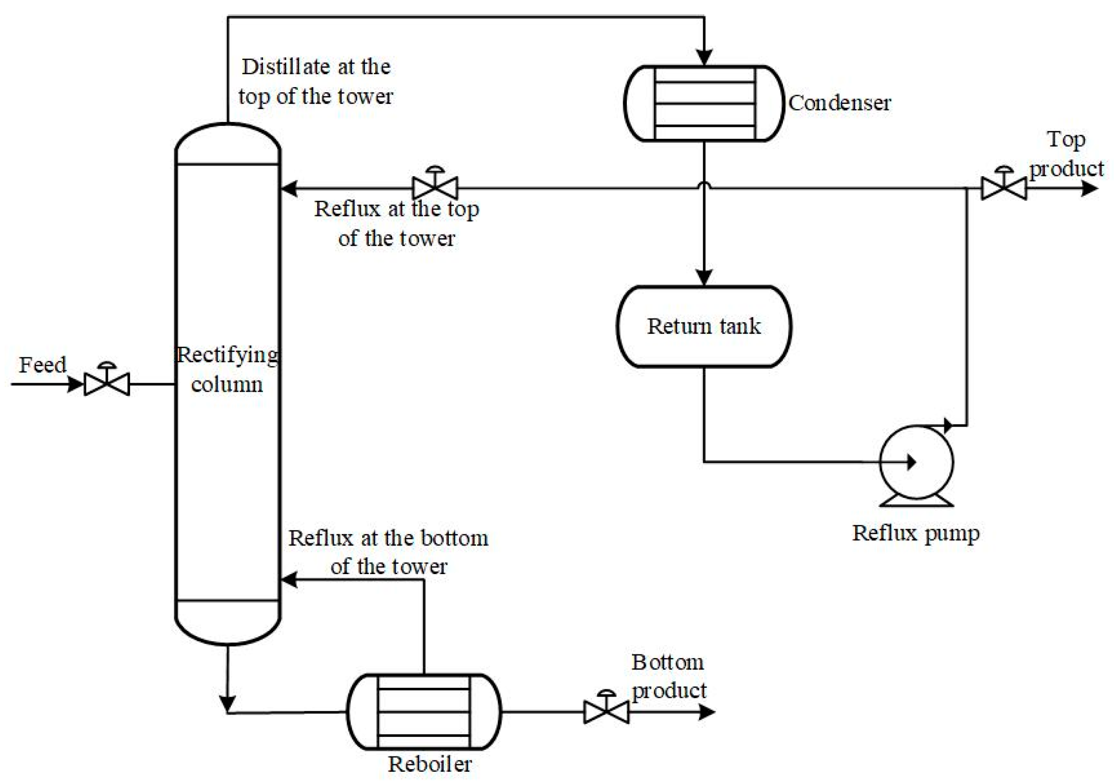
Distillation is the most widely used mass transfer operating unit in petroleum refining, petrochemical, and other industrial processes. It is also one of the most energy-intensive unit operations in petrochemicals. Figure 1 shows the structure of a typical distillation column. The energy consumption of distillation columns accounts for approximately one third of the total energy consumption of chemical plants. Statistics show that approximately 40~50% of the total energy consumption in the petroleum and chemical industry is consumed by the distillation process [1]. Therefore, improving the efficiency of the distillation process greatly impacts on the energy conservation and emission reduction of the chemical process, which cannot be realized without an efficient modeling and control method [2,3].

New process equipment design and effective control scheme are two main aspects of energy-saving research in distillation processes [4]. Many new types of distillation columns have been designed by researchers, such as the divided-wall column [5,6], the heat pump-assisted distillation column [7,8], the heat integrated distillation column [9,10], the pressure-swing distillation column with heat integration [11,12], the heat integrated extractive distillation column [13,14], and so on. Most of these columns introduce heat exchange sections to largely reuse the internal thermal cycle. Therefore, the energy utilization rate has been largely improved. However, the heat integration part makes the interaction stronger than traditional columns. Therefore, although the new part can largely improve the energy efficiency, it makes the control design more difficult. In addition, the research on energy-saving technology for processing and equipment has shortcomings, such as long cycles, large investment, and slow replacement, so it is difficult to put into commercial production in a short time [15]. To realize energy saving rapidly in a distillation process, it is necessary to strengthen the operation control. A highly effective control scheme usually relies on a nonlinear dynamic model, which must be both accurate and simplified enough.

The mechanism model is accurate enough to characterize the dynamic properties of the distillation process, and it is usually represented by differential and algebraic equations. However, a series of nonlinear differential equations with high dimension and rigidity must be solved in the modeling process of a distillation column. The size of the differential equations increases with the number of trays in the distillation column, which increases the difficulty of the online solution to the mechanism model. Therefore, it is difficult to utilize online in a control scheme for the mechanism model [16].

Many approximate linear models were investigated in distillation control design for the problem above, such as the ARX model [17], the CARIMA model [18], the internal transfer function model [19], the impulse response model [20], and so on. Manipulated variables can be easily solved out by these linear models in an online control loop. However, this oversimplified model would certainly bring in model mismatch, making the control schemes effective only in a limited operating range [21]. Once a significant disturbance is involved, the control performance will probably deteriorate. In addition, PID is the most commonly used control method for distillation columns, independent of the process model. However, PID is a linear method and, therefore, cannot process serious nonlinear problems perfectly [22], which widely exist in distillation columns.

Many researchers aim to establish an appropriate nonlinear simplified model to overcome the disadvantages of both the mechanism model and the linearization method. Among these studies, a nonlinear wave theory has provided a promising way to solve the problems above. The nonlinear wave theory was inspired by the chromatograph study by Hwang and his coworkers [23], who found that the curve of the concentration on each tray kept a relatively stable shape from the results of both simulation and experimental research. Therefore, the concentration distribution along the entire column could be regarded as a whole, which would essentially decrease the number of state variables to characterize the distillation process. Moreover, these variables could be used to establish a simplified nonlinear dynamic model [24]. In particular, this simplified nonlinear modeling method shows a decisive advantage in modeling complex chemical processes with self-organizing properties. Based on the above complex nonlinear modeling research, the concentration distribution curve and its movement characteristics in the distillation column are gradually excavated. However, some problems limit the application of this approach. First, the assumption of the stable shape of the concentration curve was established from the simulation and experiment by data analysis [25]. Second, some unrealistic assumptions were adopted to reduce the application difficulty of the theory. For example, the movement of the concentration curve was regarded as keeping a constant rate, which would not be applicable in most distillation processes. In brief, the nonlinear wave theory provides a promising solution, and some detailed assumptions can be refined to suit actual situations.

In this paper, a nonlinear dynamic model is established according to the equilibrium theory in the distillation column. Based on the equilibrium relationships in the distillation separation process, we can derive that the concentration distribution curve has a fixed descriptive function form, consistent with the simulation and experiment by Hwang. Therefore, the idea of taking the concentration distribution curve as a whole has been supported by the separation mechanism. In addition, the movement of the concentration distribution curve is re-described without the assumption of a constant moving rate, which would be more practical than the traditional nonlinear wave theory. Based on the concentration curve describing function and the moving rate description, a nonlinear dynamic model can be established. The proposed model can not only accurately describe the characteristics of the system, but also greatly simplify the structure compared with the mechanism model. Finally, a generic model control (GMC) scheme based on the proposed nonlinear model is designed for the distillation column. In the case study, the GMC controller performs better than a traditional PID control method. GMC shows good performance in both servo and regulation control. Experimental results demonstrate the effectiveness of the proposed nonlinear distillation column model and the model-based control scheme.

2. Modeling of the Distillation Column Based on the Equilibrium Theory

In the nonlinear wave theory mentioned above, the concentration distribution in the distillation column can be regarded as a whole. When the operating condition changes, the concentration curve moves along the column and behaves like wave profile propagation. For example, Figure 2 shows the movement of the concentration distribution curve along the distillation column when the feed composition Z_f increases by 5% in a distillation column with 10 trays. After the feed composition changes, the original profile 1 moves to the right in the column and finally stops at the position of profile 2, which represents a new steady state. The profile shape of the curve keeps a relatively stable structure during the process. The moving process of the concentration distribution curve represents the entire system’s dynamic response process after the change of operating conditions.

Essentially, the motion of the concentration distribution curve is a symptom of the mass transfer in the separation process. Figure 3 is a schematic diagram of the balanced relationship of a single tray. A basic assumption is adopted in the tray model that the gas and liquid phases are uniformly mixed and in thermodynamic equilibrium. The droplets in the gas phase, the bubbles in the liquid phase, and the liquid phase flowing down through the main section are ignored. The dynamics in the downpipe are not considered.

If there are enough trays in a plate distillation column, it can be assumed that the structure of the plate distillation column is similar to that of a packed column [26]. Therefore, the mass transfer partial differential equation in a minimal unit volume in the distillation process can be regarded as follows:

$$\frac{\partial x}{\partial t}-\frac{\partial x}{\partial u}=-D_T(y^{*}(x)-y)$$

(1)

$$\frac{V}{L}\frac{\partial y}{\partial u}=D_T(y^{*}(x)-y)$$

(2)

where x and y are liquid and gas phase concentrations, respectively. D_T is the dimensionless mass transfer coefficient, L is the liquid molar flow rate, V is the gas molar flow rate, $y^{*}(x)$ describes the gas-liquid equilibrium relationship, and u is the dimensionless space coordinate variable.

Suppose that the process is in a quasi-steady state where ∂x/∂t = 0. Then, transform the original coordinate system into a $l-t$ coordinate system with a velocity of v to better explain the idea of the concentration curve and its motion as a whole. Let the coordinates transform as follows:

$$l=u-u^{\prime }$$

(3)

$$u^{\prime }={\displaystyle \int vdt}$$

(4)

Substituting Equations (3) and (4) into Equations (1) and (2), we can get:

$$(1+v)\frac{\partial x}{\partial l}=D_T(y^{*}(x)-y)$$

(5)

$$\frac{V}{L}(1+v)\frac{\partial y}{\partial l}=D_T(y^{*}(x)-y)$$

(6)

where $u=u^{\prime }$ is the origin of the new coordinate of $l-t$.

According to Equations (5) and (6), the following equation can be obtained:

$$l-{\displaystyle \int \frac{(1+v)dx}{D_T(C_1+y^{*}(x)-Lx/V)}}+C_2=0$$

(7)

where C₁ and C₂ are the constant terms generated by the indefinite integration of Equations (5) and (6). To simplify the derivation, a second-order polynomial y^*(x) = ax² + bx + c is used to approximate the gas-liquid equilibrium relation y^*(x). The integrand in Equation (7) can be expressed in a concise form:

$$\frac{(1+v)}{D_T(C_1+y^{*}(x)-Lx/V)}=\frac{1}{q_3(x-q_1)(x-q_2)}$$

(8)

where $q_1$, $q_2$, and $q_3$ are equivalent parameters generated by factorization. Therefore, the analytical solution of the concentration distribution can be integrated by plugging Equation (8) into Equation (7):

$$X\left(l\right)=q_2+\frac{q_1-q_2}{1+e^{q_3(q_1-q_2)(l-q_4)}}$$

(9)

where $q_4$ is a constant term generated by the integration.

According to Equation (9), the concentration distribution of each tray has a fixed descriptive function form. The parameters ($q_1$, $q_2$, $q_3$ and $q_4$) in the formula would certainly vary with time during a dynamic process, but the formula structure does not change. Now, we transform the system from the new coordinate to the old one. Letting $S=u^{\prime }+q_4$, β = q₃(q₂ − q₁), we can obtain the description function of the concentration distribution:

$$X\left(u\right)=q_2+\frac{q_1-q_2}{1+e^{-\beta (u-S)}}$$

(10)

In the process of distillation separation, the middle part of the profile shape in the dynamic process is basically in a quasi-steady state, and q₄ changes little over time. Therefore, the moving velocity of the distribution curve can be represented by the velocity of the position S (S is called the inflection point of the concentration distribution curve):

$$\frac{dS}{dt}=\frac{d{u}^{\prime }}{dt}=v$$

(11)

The distribution parameters, q₁, q₂, and β, have practical physical significance in the distribution description function. q₁ and q₂ are the maximum and minimum approximations of the distribution description function, and β represents the slope of the inflection point. Therefore, the concentration distribution description function of the rectifying and stripping sections in a plate column can be obtained as follows:

$${\widehat{X}}_j=X_{r\_\min }+\frac{X_{r\_\max }-X_{r\_\min }}{1+e^{-k_r(j-S_1)}}\hspace{1em}j=1,2,\cdots ,f-1$$

(12)

$${\widehat{X}}_j=X_{s\_\min }+\frac{X_{s\_\max }-X_{s\_\min }}{1+e^{-k_s(j-S_2)}}\hspace{1em}j=f,f+1,\cdots ,n$$

(13)

where ${\widehat{X}}_j$ is the estimated concentration value on the jth tray. X_{r_max}, X_{r_min}, k_r, X_{s_max}, X_{s_min}, and k_s are the concentration distribution parameters. f is the feed tray, and n is the total number of trays. Note that the functions of the rectifying and stripping sections are described separately since the feed may influence the continuity of the concentration curve.

The parameters of the concentration distribution have physical significance, as mentioned above. X_{r_max} and X_{s_max} are the maximum approximate concentrations of the rectifying and stripping sections, respectively. X_{r_min} and X_{s_min} are the minimum approximate concentrations of the rectifying section and the stripping section, respectively. k_r and k_s represent the slope at the inflection point. For an intuitive representation, Case 2 in Section 3 is taken as an example here to describe the concentration distribution in the initial steady state and its expansion curve in the rectifying section and the stripping section, as shown in Figure 4.

Figure 5 shows the estimated errors of liquid component concentrations predicted by Equations (12) and (13). The parameters are determined by a simple least squares method. The largest prediction error is approximately 1 × 10⁻³, mainly around the feed tray with a strong interference factor. The results show that the solution by Equations (12) and (13) can be used to describe the shape of the distribution curve with relatively high precision.

By differentiating both sides of Equations (12) and (13), the relation between the component concentration and the moving velocity of the distribution curve (the velocity of the inflection points) can be obtained:

$$\frac{{d \widehat{X}}_j}{dt}=\frac{-k_r(X_{r\_\max }-X_j)(X_j-X_{r\_\min })}{X_{r\_\max }-X_{r\_\min }}\frac{d{S}_1}{dt}$$

(14)

$$\frac{{d \widehat{X}}_j}{dt}=\frac{-k_s(X_{s\_\max }-X_j)(X_j-X_{s\_\min })}{X_{s\_\max }-X_{s\_\min }}\frac{d{S}_2}{dt}$$

(15)

where we ignore the variation with time of the parameters since they change very slow during a dynamic process.

The material conservation relationships of each tray of the distillation column are shown as follows:

$$M_1\frac{d{X}_1}{dt}=V{Y}_2-(L+D)X_1$$

(16)

$$M\frac{d{X}_j}{dt}=L(X_{j-1}-X_j)+V(Y_{j+1}-Y_j),j=2,\dots ,f-1$$

(17)

$$M\frac{d{X}_f}{dt}=F{Z}_f+L{X}_{f-1}-L_1{X}_f+V_1{Y}_{f+1}-V{Y}_f$$

(18)

$$M\frac{d{X}_j}{dt}=L_1(X_{j-1}-X_j{)+V}_1(Y_{j+1}-Y_j),j=f+1,\dots ,n-1$$

(19)

$$M_B\frac{d{X}_n}{dt}=L_1{X}_{n-1}-V_1{Y}_n-W{X}_n$$

(20)

where M₁, M, and M_B are the liquid holdings of the top of the column, each tray, and the bottom of the column, respectively, F is the feed flow rate, and Z_f is the feed composition. The liquid flow rate is L and the gas flow rate is V. D and W are the product quantities of the top and bottom of the column, respectively, and Y is the concentration of the light component in the gas phase.

The gas-liquid molar flow rate is calculated according to mass conservation as follows:

$$V=V_1-F(1-q)$$

(21)

$$L=V-D$$

(22)

$$L_1=L+F$$

(23)

where V₁ is the gas molar flow rate in the stripping section, L₁ is the liquid molar flow rate in the stripping section, and q is feed thermal condition.

The calculation formula of the product quantity at the top and bottom of the column is:

$$D=V/(R+1)$$

(24)

$$W=L_1-V_1$$

(25)

where R is the rflux ratio.

The concentration of the light component in the gas phase can be calculated by the gas-liquid equilibrium relationship in an ideal mixture separation system:

$$Y_j=\frac{\alpha X_j}{(\alpha -1)X_j+1},j=1,2,\dots ,n$$

(26)

where, α is the relative volatility.

We plug Equations (14) and (15) into Equations (16)–(20), and the trays in the rectifying section and the stripping section are summed up, respectively. Then, the moving velocity formula of the concentration distribution curve of the distillation column can be obtained through an algebraic transformation as follows:

$$\frac{d{S}_1}{dt}=\frac{(\frac{Y_2-X_1}{M_1}+\frac{Y_f-Y_2}{M})V_1+\frac{L(X_1-X_{f-1})}{M}}{-{\displaystyle \sum _{j=1}^{f-1}\frac{kr(X_{r\_\max }-X_j)(X_j-X_{r\_\min })}{X_{r\_\max }-X_{r\_\min }}}}$$

(27)

$$\frac{d{S}_2}{dt}=\frac{(\frac{Y_n-Y_f}{M}+\frac{X_n-Y_n}{M_B})V_1+(\frac{X_{f-1}-X_{n-1}}{M}+\frac{X_{n-1}-X_n}{M_B})L+\frac{F(Z_f-X_{n-1})}{M}+\frac{F(X_{n-1}-X_n)}{M_B}}{-{\displaystyle \sum _{j=f}^n\frac{ks(X_{s\_\max }-X_j)(X_j-X_{s\_\min })}{X_{s\_\max }-X_{s\_\min }}}}$$

(28)

In conclusion, the nonlinear dynamic model of a distillation column can be established based on the equilibrium theory, including the moving velocity of the concentration distribution curve (Equations (27) and (28)), the description functions of the concentration distribution curve (Equations (12) and (13)), the gas-liquid equilibrium (Equation (26)), the gas-liquid molar flow calculation (Equations (21)–(23)), and the product quantity at the top and bottom trays of the distillation column (Equations (24) and (25)). The simulation is carried out in Matlab 2019b. In the simulation solving process, the initial values of critical variables should be provided first, such as the position of the inflection point and the profile parameters. Then, based on the algebraic and differential equations listed above, a basic Euler method can be applied to solve this DAE problem.

The proposed nonlinear dynamic model removes the material conservation differential equations compared with the mechanism model. Two differential variables are added, namely the velocities of the inflection points of the rectifying section and the stripping section. The specific comparison is shown in

Table 1. Comparison between the number of differential equations and state variables.

	Number of Differential Equations	Number of State Variables
Mechanism model	n	n
Model of this paper	2	2

. Reducing the number of differential equations and variables simplifies the structure of the nonlinear model, making online solution and control design more convenient.

3. Model Test

The nonlinearity of the distillation column will be enhanced with the increase in the trays. Therefore, to comprehensively test the model’s accuracy, we take two benzene-toluene (CAS No.71-43-2 and 108-88-3, respectively) systems with different trays as simulation experiments. There are 10 trays in the distillation column of Case 1 and 20 trays in Case 2 [27]. Suppose that the resistance of mass and heat transfer between the gas and liquid phases on the tray is zero, and when they are fully mixed reach the equilibrium state.

3.1. Case 1

The specific operating conditions of Case 1 are shown in

Table 2. Operating conditions of the distillation column in Case 1.

Operating Conditions	Value	Operating Conditions	Value
Feed flow rate F (kmol/h)	40	Feed composition Zf (benzene)	0.6
Reflux ratio R	5	Liquid holdup at the top of the tower M1 (kmol)	75
Feed stage f	5	Liquid holdup in each stage M (kmol)	10
Stage number n	10	Liquid holdup at the bottom of the tower MB (kmol)	150
Feed thermal condition q	1	Relative volatility α	2.317
Temperature of feed (°C)	20	Pressure (kpa)	101.3

. Figure 6 shows the concentration distribution of the distillation column when it reaches a steady state under the above operating conditions. The purity of benzene at the top of the column is 94.5%, and benzene at the bottom of the column is 2.5%.

Figure 7 and Figure 8 show the concentration tracking errors between the proposed model and the mechanism model on the first tray and the n-th tray when the feed flow rate F and the feed composition Z_f are increased by a step of 10%, respectively. As shown in the figures, the magnitude order of the errors stays in the range of 10⁻⁵~10⁻⁶, and the errors occur mainly at the beginning of the dynamic process and then approach zero gradually. Therefore, the tracking errors have little influence on the overall stability of the dynamic model, and the model has a high concentration observation accuracy.

3.2. Case 2

The operating conditions of Case 2 are shown in

Table 3. Operating conditions of the distillation column in Case 2.

Operating Conditions	Value	Operating Conditions	Value
Feed flow rate F (kmol/h)	100	Feed composition Zf	0.55
Reflux ratio R	1.7	Liquid holdup at the top of the tower M1 (kmol)	75
Feed stage f	11	Liquid holdup in each stage M (kmol)	10
Stage number n	20	Liquid holdup at the bottom of the tower MB (kmol)	150
Feed thermal condition q	1	Relative volatility α	2.317
Temperature of feed (°C)	20	Pressure (kpa)	101.3

. The distillation column in this case has stronger nonlinearity due to the increase in the number of trays. The purity of benzene at the top of the column is 98%, and benzene at the bottom of the column is 1.2%.

In the proposed modeling theory, the dynamic properties of the systems are represented by the change of the inflection point position and the change of the moving velocity of the concentration distribution curve. The accuracy of the dynamic model is ultimately reflected in the tracking of the concentration variation.

First, we test the concentration observation results of the dynamic model at several trays numbered 1, 7, 13, and 20 when the feed flow rate F is increased by 10%, as shown in Figure 9. As shown in the figure, during the whole dynamic change process, the observed concentration of the proposed model can track the change of the actual concentration of the column accurately, especially at the top and bottom of the column, where the two curves almost coincide. The results show that the established dynamic model can well reflect the dynamic characteristics of the system under the change of the feed flow rate.

Figure 10 records the concentration observation of the dynamic model in the distillation column under the step change of the feeding composition Z_f. It can be seen that the system has a pronounced fluctuation process. The situations are similar to the responses when F increases, except for the situation at the 13th tray. The 13th tray in the stripping section is close to the feed tray and therefore is easily interfered with by the feed flow. This factor leads to an obvious difference between the observed value and the actual value of the tray. However, the variation trend of the concentration is well depicted by the proposed model. The dynamic model can maintain high-precision concentration prediction at most of the trays, especially the top and bottom trays of the column, which are more critical in the control design than other trays.

4. Generic Model Control Based on the Nonlinear Dynamic Model

4.1. The Principle of Generic Model Control

Generic model control (GMC) has the advantages of simple control structure, excellent nonlinear control performance, and easy parameter tuning, and is widely used in various fields [28,29]. In the GMC control scheme design of a distillation column, it is necessary to ensure that the concentrations at the top and bottom of the column reach their set values. Based on the proposed nonlinear model, the control of the top and bottom concentrations can be equivalent to the positions of the inflection points in the rectifying and stripping sections, respectively, because the concentration curve keeps a relatively unchanged shape. Therefore, the concentrations at both ends should have a certain relationship to the inflection points at the middle part of the curve according to Equations (12) and (13). In the proposed model, the velocities of the inflection points are specific, as depicted in Equations (27) and (28), which represent the derivative of the inflection point positions. The GMC controller can effectively control the derivative of the controlled variable to achieve the requirements. Therefore, GMC can be directly embedded into the nonlinear model without introducing other approximation links, which significantly improves the robustness and effectiveness of the control scheme.

For the following nonlinear model:

$$\frac{dx}{dt}=f(x,u,d,t)$$

(29)

$$y=g(x)$$

(30)

where x is the state variable, u is the control variable, d is the interference variable, and y is the output variable. The functions f and g represent nonlinear functional relations.

From Equations (29) and (30), we can obtain:

$$\dot{y}=G_{x}f(x,u,d,t)$$

(31)

where $G_x=\frac{\partial g}{\partial x}$.

When the output variable of the system deviates from its set value y*, we calculate the rate of the change of y, that is ${\dot{y}}^{*}$, to make the system return to the steady state:

$${\dot{y}}^{*}=K_1(y^{*}-y)$$

(32)

where K₁ is the controller parameter.

If we want to ensure that the final controlled variable has no residual difference, the objective function relationship should include an integral part:

$${\dot{y}}^{*}=K_1(y^{*}-y)+K_2{\displaystyle \int (y^{*}-y)dt}$$

(33)

where K₂ is the controller parameter.

By substituting the above formula into Equation (31), we can obtain:

$$G_{x}f(x,u,d,t)=K_1(y^{*}-y)+K_2{\displaystyle \int (y^{*}-y)dt}$$

(34)

In order to realize the control law, the approximate model of a complex process is usually utilized, and Equation (34) is converted into the following equation:

$${\widehat{G}}_x\widehat{f}(x,u,d,t)=K_1(y^{*}-y)+K_2{\displaystyle \int (y^{*}-y)dt}$$

(35)

where $\widehat{f}$ and ${\widehat{G}}_x$ are approximate simple function relations of the process and the effect of GMC largely depends on the concrete realization form of $\widehat{f}$ and ${\widehat{G}}_x$. The errors of the approximate model would certainly exist. Therefore, the control function contains integral terms, which can effectively weaken the influence of errors.

4.2. Generic Model Control Design of the Distillation Column

In the proposed distillation column model, the movement of the inflection point can effectively represent the transition process. The concentration of the top and bottom trays are the controlled variables, and they can be controlled indirectly by direct control of the positions of the inflection points, S₁ and S₂. Reflux ratio R and gas flow rate V₁ in the distillation section are taken as manipulated variables.

According to the GMC algorithm, there are the following expressions:

$$\frac{d{S}_1}{dt}=K_{11}(S_1{}^{*}-S_1)+K_{12}{\displaystyle {\int }_0^t(S_1{}^{*}-S_1})dt$$

(36)

$$\frac{d{S}_2}{dt}=K_{21}(S_2{}^{*}-S_2)+K_{22}{\displaystyle {\int }_0^t(S_2{}^{*}-S_2})dt$$

(37)

where K₁₁, K₁₂, K₂₁, and K₂₂ represent adjustable parameters in GMC, and subscripts 1, 2 represent the rectifying and stripping sections, respectively. S₁* and S₂* are the set values of the inflection point in the rectifying and stripping units, respectively. Combined with the moving velocities of the concentration distribution curves introduced above (Equations (27) and (28)), we can obtain:

$$K_{11}(S_1{}^{*}-S_1)+K_{12}{\displaystyle {\int }_0^t(S_1{}^{*}-S_1)dt=}\frac{(\frac{Y_2-X_1}{M_1}+\frac{Y_f-Y_2}{M})V_1+\frac{L(X_1-X_{f-1})}{M}}{-{\displaystyle \sum _{j=1}^{f-1}\frac{kr\left(X_{r\_\max }-X_j\right)\left(X_j-X_{r\_\min }\right)}{X_{r\_\max }-X_{r\_\min }}}}$$

(38)

$$K_{21}(S_2{}^{*}-S_2)+K_{22}{\displaystyle {\int }_0^t(S_2{}^{*}-S_2)dt}=\frac{(\frac{Y_n-Y_f}{M}+\frac{X_n-Y_n}{MB})V_1+(\frac{X_{f-1}-X_{n-1}}{M}+\frac{X_{n-1}-X_n}{MB})L+\frac{F(Z_f-X_{n-1})}{M}+\frac{F(X_{n-1}-X_n)}{MB}}{-{\displaystyle \sum _{j=f}^n\frac{ks(X_{s\_\max }-X_j)(X_j-X_{s\_\min })}{X_{s\_\max }-X_{s\_\min }}}}$$

(39)

Then, based on the other equations of the proposed model, the control variables (the reflux ratio R and the gas flow rate V₁ in the stripping section) can be solved out. The specific control structure is shown in Figure 11.

4.3. Simulation Case 1

First, we take the example in Case 1 as the research object to carry out the control simulation experiment. The GMC controller based on the equilibrium theory model is compared with a traditional PID controller. The PID control scheme adopts proportional and integral control (PI controller), including two loops, respectively, to control the product concentration at the top and the bottom of the column. It is assumed that the set value of the concentration at the top of the column is Y1*, and the set value at the bottom is Xn*. To clearly represent the changes of controlled variables, the ordinate in the resulting chart is expressed as follows: ΔY1 = Y1 − Y1*, ΔXn = Xn − Xn*.

4.3.1. Servo Control

Figure 12 shows the response curve when the set value at the top and the bottom of the column changes. The concentration set value at the top of the column has a step change from 0.945 to 0.94, while the concentration set value at the bottom has a step change from 0.025 to 0.024. As shown in the figure, both GMC and PID finally have no offsets, and no obvious oscillation occurs. However, the stability time of GMC at the top and the bottom of the column is 5.5 h and 6 h, respectively, while PID takes approximately 19 h. Therefore, GMC has apparent advantages over PID at both the top and the bottom of the column.

4.3.2. Regulatory Control

Figure 13 and Figure 14 show the responses at the top and bottom trays when feed flow rate F and feed composition Z_f increase by 20%, respectively. As shown in the figures, the GMC control strategy based on the equilibrium theory model can effectively eliminate the influence of disturbances, and the adjustment time is approximately 5 h. Compared with PID, GMC has the advantages of fast response speed and slight overshoot. Therefore, GMC has shown excellent control performance.

4.3.3. Regulatory Control

To clearly represent the changes in the controlled variables, the absolute integral error (IAE) and the square integral error (ISE) are used as error quantification standards. The calculation formula is as follows:

$$IAE=\frac{1}{n_t}{\displaystyle \sum _{k=1}^{n_t}|x(k)-x^{*}}|$$

(40)

$$ISE=\frac{1}{n_t}{\displaystyle \sum _{k=1}^{n_t}{(x(k)-x^{*})}^2}$$

(41)

where n_t is the total sampling times, x(k) is the controlled variable, which in this paper is Y₁ or X_n, and x* corresponds to the set value of the controlled variable.

Table 4. Error index of GMC in Case 1.

	Servo Control	F+20%	Zf+20%
IAE_Y1	3.80 × 10−4	1.28 × 10−5	9.48 × 10−5
IAE_Xn	1.24 × 10−4	6.71 × 10−5	6.63 × 10−5
ISE_Y1	1.36 × 10−6	1.13 × 10−9	5.67 × 10−8
ISE_Xn	1.07 × 10−7	5.31 × 10−8	3.92 × 10−8

and

Table 5. Error index of PID in Case 1.

	Servo Control	F+20%	Zf+20%
IAE_Y1	7.94 × 10−4	1.14 × 10−4	4.91 × 10−4
IAE_Xn	2.58 × 10−4	2.10 × 10−4	2.06 × 10−4
ISE_Y1	2.44 × 10−6	5.37 × 10−8	1.08 × 10−6
ISE_Xn	1.56 × 10−7	2.59 × 10−7	1.41 × 10−7

show the error indexes of GMC and PID, respectively. It can be seen from the error index that the servo control and feed composition disturbance have a greater influence on the entire system than the feed flow rate disturbance. Generally speaking, the control effect of GMC is obviously better than PID in all aspects.

4.4. Simulation Case 2

Similar to Case 1, we take a benzene-toluene separation distillation with 20 trays (the same as Case 2 in Model Test) in Case 2 as the research object to conduct the simulation experiment. The same PID control strategy as Case 1 is utilized to compare with GMC.

4.4.1. Servo Control

Figure 15 shows the comparison of controlled variable responses of the two control schemes when the set value at the top of the column changes by a step from 0.98 to 0.992, and the set value at the bottom changes by a step from 0.012 to 0.0132. It can be seen from the figure that the fluctuation of GMC is obviously stronger than PID in this servo control. GMC stabilizes at the top and the bottom of the column after 3 h and 1.8 h, respectively, while PID takes approximately 4.5 h to complete concentration track. Therefore, GMC, based on the equilibrium theory model, has a faster response speed, and the tracking effect is better than PID.

To make a more precise comparison between the two controllers, we retune the parameters of PID and try to make the responses of the top tray basically consistent with each other, as shown in Figure 16. It can be observed from the figure that the control effect of PID at the top of the column is similar to that of GMC, but at the bottom of the column, PID deteriorates significantly, where the response cannot reach a stable state for a long time. Due to the nonlinearity and interaction of the process, if PID achieves the same control effect as GMC at the top of the column, the control effect at the bottom of the column cannot be guaranteed. Therefore, PID cannot consider both ends at the same time, so a compromise must be made between the top and bottom trays when tuning the parameters of PID. If the elimination of the offset at both ends has a priority, the response speed would be sacrificed, as shown in Figure 15. On the contrary, if the response speed has to be considered first, the system would oscillate for a long time, as shown in Figure 16. Considering that stability is more important, PID in Figure 15 is preferred, compared with that in Figure 16. In contrast, GMC can make a good balance between control accuracy and speed.

4.4.2. Regulatory Control

Figure 17 shows the response curve comparison between the two control schemes when the feed flow rate F increases by 20%. Under the disturbance of the feed flow rate, the PID control effect decreases seriously. Especially in the rectifying section, the oscillation is strong, and the controlled variable cannot be stabilized around the set value for a long time. The control effect of GMC is obviously better than PID, the overall oscillation amplitude is smaller, especially in the stripping section, and the stabilization speed is faster. Compared with PID, the overshoot and fluctuation can be almost ignored, and the controlled variables are always maintained around the set values.

Figure 18 compares the two control schemes under the disturbance of a 20% increase in feed composition Z_f. The control effect of GMC is obviously better than that of PID, and the overshoot amplitude is much smaller than that of PID. The rectifying and stripping sections can reach the new set value in approximately 1.6 h. PID oscillates for a long time in the stripping section, the influence of disturbance cannot be completely eliminated, and the fluctuation is pronounced.

4.4.3. Error Index Analysis

Similarly,

Table 6. Error index of GMC in Case 2.

	Servo Control	F+20%	Zf+20%
IAE_Y1	5.74 × 10−5	6.26 × 10−7	1.38 × 10−5
IAE_Xn	7.79 × 10−5	1.31 × 10−5	2.97 × 10−5
ISE_Y1	1.44 × 10−8	1.11 × 10−12	7.59 × 10−10
ISE_Xn	4.84 × 10−8	1.08 × 10−9	4.98 × 10−9

and

Table 7. Error index of PID in Case 2.

	Servo Control	F+20%	Zf+20%
IAE_Y1	1.51 × 10−4	2.39 × 10−6	5.28 × 10−5
IAE_Xn	3.22 × 10−4	1.81 × 10−4	1.05 × 10−4
ISE_Y1	4.42 × 10−8	1.41 × 10−11	5.18 × 10−9
ISE_Xn	2.18 × 10−7	1.25 × 10−7	3.18 × 10−8

show the error indexes of GMC and PID in Case 2, respectively. Since PID has a long-term oscillation that is difficult to eliminate in many cases, the gap of the indicators between PID and GMC is obvious. Generally, GMC has a better control performance owing to the proposed nonlinear model.

5. Conclusions

In this paper, the mass transfer mechanism of the distillation process is carefully studied and a concentration distribution function is obtained based on the equilibrium theory, including gas-liquid equilibrium, mass balance, and component equilibrium. From the derivation, the overall concentration distribution curve is in a relatively stable profile shape and can be described by a specific function structure. Then, the moving velocity of the concentration distribution curve was derived, and the nonlinear dynamic model of the distillation process was established on this basis. The proposed model can largely reduce the model size of the mechanism model and, meanwhile, capture the dynamic characteristics of the nonlinear distillation process well. In the dynamic simulation test of two benzene-toluene separation cases, the model established in this paper was compared with the mechanism model when operating condition changes are involved. The test results show that the model can accurately track the differences in each tray’s actual values. Finally, to embed the established nonlinear equilibrium theory model into an online control algorithm, we introduced generic model control (GMC) algorithm and conducted two simulation studies. Compared with a traditional PID control scheme, the responses and error indicators show that the model-based GMC has significant advantages in both servo and regulatory control studies. The simulation also proves the validity of our proposed nonlinear model.

This work provides a new mechanism modeling method for distillation columns, especially for model-based online approaches. Note that the conclusions are derived based on an approximate gas-liquid equilibrium function and an ideal system of benzene-toluene separation is utilized to prove the validity of the model. The applicability of the proposed model in non-ideal systems needs further study. In addition, side feeds or withdrawals in the middle part of the column may affect the integrity and continuity of the concentration distribution curve. Future work should focus on accurately describing the gas-liquid equilibrium relation and developing applicable nonlinear models for complex distillation systems.

References

- Kiss, A.A. Distillation technology-still young and full of breakthrough opportunities. J. Chem. Technol. Biot. 2014, 89, 479–498. [Google Scholar] [CrossRef]
- Jana, A.K. Heat integrated distillation operation. Appl. Energy 2010, 87, 1477–1494. [Google Scholar] [CrossRef]
- Carrasco, B.; Avila, E.; Viloria, A.; Ricaurte, M. Shrinking-Core Model Integrating to the Fluid-Dynamic Analysis of Fixed-Bed Adsorption Towers for H2S Removal from Natural Gas. Energies 2021, 14, 5576. [Google Scholar] [CrossRef]
- Ye, Q.; Wang, Y.; Pan, H.; Zhou, W.; Yuan, P. Design and Control of Extractive Dividing Wall Column for Separating Dipropyl Ether/1-Propyl Alcohol Mixture. Processes 2022, 10, 665. [Google Scholar] [CrossRef]
- Aurangzeb, M.; Jana, A.K. A Novel Heat Integrated Extractive Dividing Wall Column for Ethanol Dehydration. Ind. Eng. Chem. Res. 2019, 58, 9109–9117. [Google Scholar] [CrossRef]
- Tian, Y.; Meduri, V.; Bindlish, R.; Pistikopoulos, E.N. A Process Intensification synthesis framework for the design of dividing wall column systems. Comput. Chem. Eng. 2022, 160, 107679. [Google Scholar] [CrossRef]
- Jana, A.K.; Mane, A. Heat Pump Assisted Reactive Distillation: Wide Boiling Mixture. AIChE J. 2011, 57, 3233–3237. [Google Scholar] [CrossRef]
- Lu, L.; Hua, G.; Tao, J.; Chen, Y.; Zhang, Y.; Shen, W. An energy sustainable approach of heat-pump assisted azeotropic divided wall column based on the organic Rankine cycle. Braz. J. Chem. Eng. 2022, 39, 539–552. [Google Scholar] [CrossRef]
- Li, T.; Fu, S.; Zhang, Z.; Sun, J. Utilizing heat sinks for further energy efficiency improvement in multiple heat integrated five-column methanol distillation scheme. Chem. Eng. Process. 2017, 121, 65–70. [Google Scholar] [CrossRef]
- Javed, A.; Hassan, A.; Babar, M.; Azhar, U.; Riaz, A.; Mujahid, R.; Ahmad, T.; Mubashir, M.; Lim, H.R.; Show, P.L.; et al. A Comparison of the Exergy Efficiencies of Various Heat-Integrated Distillation Columns. Energies 2022, 15, 6498. [Google Scholar] [CrossRef]
- Li, Y.; Jiang, Y.; Xu, C. Robust Control of Partially Heat-Integrated Pressure-Swing Distillation for Separating Binary Maximum-Boiling Azeotropes. Ind. Eng. Chem. Res. 2019, 58, 2296–2309. [Google Scholar] [CrossRef]
- Chen, Y.; Liu, C.; Geng, Z. Design and control of fully heat-integrated pressure swing distillation with a side withdrawal for separating the methanol/methyl acetate/acetaldehyde ternary mixture. Chem. Eng. Process. 2018, 123, 233–248. [Google Scholar] [CrossRef]
- Cui, F.; Cui, C.; Sun, J. Simultaneous Optimization of Heat-Integrated Extractive Distillation with a Recycle Feed Using Pseudo Transient Continuation Models. Ind. Eng. Chem. Res. 2018, 57, 15423–15436. [Google Scholar] [CrossRef]
- Jian, X.; Li, J.; Ye, Q.; Yan, L.; Li, X.; Zhang, J. Process synthesis of intensified extractive distillation for recycling organics material from wastewater. Sep. Purif. Technol. 2022, 303, 122172. [Google Scholar] [CrossRef]
- Kong, Z.Y.; Sanchez-Ramirez, E.; Yang, A.; Shen, W.; Gabriel Segovia-Hernandez, J.; Sunarso, J. Process intensification from conventional to advanced distillations: Past, present, and future. Chem. Eng. Res. Des. 2022, 188, 378–392. [Google Scholar] [CrossRef]
- Cong, L.; Xu, L.Q.; Liu, X.G. Adaptive Temperature Control for Distillation Columns Based on Relative Stability in the Profile Pattern. Ind. Eng. Chem. Res. 2021, 60, 514–527. [Google Scholar] [CrossRef]
- Liu, X.G.; Wang, C.Y.; Cong, L. Adaptive Robust Generic Model Control of High-Purity Internal Thermally Coupled Distillation Column. Chem. Eng. Technol. 2011, 34, 111–118. [Google Scholar] [CrossRef]
- Liu, X.G.; Wang, C.Y.; Cong, L.; Ding, F. Adaptive generalised predictive control of high purity internal thermally coupled distillation column. Can. J. Chem. Eng. 2012, 90, 420–428. [Google Scholar] [CrossRef]
- Zhu, Y.; Liu, X.G. Dynamics and control of high purity heat integrated distillation columns. Ind. Eng. Chem. Res. 2005, 44, 8806–8814. [Google Scholar] [CrossRef]
- Mahindrakar, V.; Hahn, J. Model predictive control of reactive distillation for benzene hydrogenation. Control Eng. Pract. 2016, 52, 103–113. [Google Scholar] [CrossRef]
- Cong, L.; Liu, X. Temperature profile movement investigation and application to a control scheme with corrected set-point for a heat integrated distillation column. Chem. Eng. Process. 2020, 147, 107710. [Google Scholar] [CrossRef]
- Jana, A.K.; Banerjee, S. Neuro estimator-based inferential extended generic model control of a reactive distillation column. Chem. Eng. Res. Des. 2018, 130, 284–294. [Google Scholar] [CrossRef]
- Hwang, Y.L.; Helfferich, F.G. Nonlinear-Waves and Asymmetric Dynamics of Countercurrent Separation Processes. AIChE J. 1989, 35, 690–693. [Google Scholar] [CrossRef]
- Hwang, Y.L. Nonlinear-Wave Theory for Dynamics of Binary Distillation-Columns. AIChE J. 1991, 37, 705–723. [Google Scholar] [CrossRef]
- Hwang, Y.L.; Graham, G.K.; Keller, G.E.; Ting, J.; Helfferich, F.G. Experimental study of wave propagation dynamics of binary distillation columns. AIChE J. 1996, 42, 2743–2760. [Google Scholar] [CrossRef]
- Marquardt, W.; Amrhein, M. Development of a Linear Distillation Model from Design-Data for Process-Control. Comput. Chem. Eng. 1994, 18, S349–S353. [Google Scholar] [CrossRef]
- Ingham, J.; Dunn, I.J.; Heinzle, E.; Prenosil, J.E. Chemical Engineering Dynamics; Wiley-VCH: Weinheim, Germany, 2000; p. 293. [Google Scholar]
- Lee, P.L.; Sullivan, G.R. Generic Model Control (Gmc). Comput. Chem. Eng. 1988, 12, 573–580. [Google Scholar] [CrossRef]
- Prakash, K.J.J.; Patle, D.S.; Jana, A.K. Neuro-estimator based GMC control of a batch reactive distillation. Isa T. 2011, 50, 357–363. [Google Scholar] [CrossRef]
Figure 1.
Structure of the distillation column.
Figure 2.
The movement of concentration distribution curve when Zf+5%.
Figure 3.
Model diagram of a single tray.
Figure 4.
Concentration distribution curve and its expansion curve.
Figure 5.
The observed error of the function described by the concentration distribution.
Figure 6.
Concentration distribution curve of distillation column in steady state.
Figure 7.
Dynamic tracking error of concentration at the top and bottom of the column when F+10%.
Figure 8.
Dynamic tracking error of concentration at the top and bottom of the column when Zf+10%.
Figure 9.
Dynamic tracking of product concentration at the 1st, 7th, 13th and 20th trays when F+10%.
Figure 10.
Dynamic tracking of product concentration at the 1st, 7th, 13th and 20th trays when Zf+10%.
Figure 11.
GMC control structure based on the proposed model.
Figure 12.
Servo response curve at top and bottom of tower.
Figure 13.
Response curve of controlled variable when the feed flow rate F+20% in Case 1.
Figure 14.
Response curve of controlled variable when the feed composition Zf+20% in Case 1.
Figure 15.
Servo response curve at the top and bottom of the tower.
Figure 16.
Figure 17.
Response curve of controlled variable when the feed flow rate F+20% in Case 2.
Figure 18.
Response curve of controlled variable when the feed composition Zf+20% in Case 2.