CFD Analysis of the Pressure Drop Caused by the Screen Blockage Rate in a Membrane Strainer

Korea Water Resources Corporation, 125, Yuseong-daero 1689beon-gil, Yuseong-gu, Daejeon 34045, Republic of Korea
*
Author to whom correspondence should be addressed.
Processes 2024, 12(4), 831; https://doi.org/10.3390/pr12040831
Submission received: 28 February 2024
/
Revised: 8 April 2024
/
Accepted: 12 April 2024
/
Published: 19 April 2024
(This article belongs to the Section Materials Processes)
Abstract
:Autostrainer is used for the purpose of debris removal in order to increase the efficiency of the heat exchanger by taking the required raw water as a heat source for the pre-cooling hydrothermal system. During the operation of the autostrainer, a pressure drop occurs due to the blockage of the screen in the autostrainer. As a result, the resistance of the pipe network for the intake system is changed, and the operating efficiency point of the pump, valve, heat exchanger, etc., is altered. By calculating the system resistance taking into account the pressure drop caused by the blockage rate of the screen in the autostrainer, the optimum operating efficiency can be expected when the intake system such as a pump, valve or heat exchanger, etc. is constructed. In this study, Computational Fluid Dynamics (CFD) was used to construct a scenario in which screen blockage may occur, predicting pressure drop for the slot cross-section of the screen in the autostrainer to derive a resistance coefficient value. The resistance coefficient value was applied to the porous region corresponding to the screen in the autostrainer’s 3D shape and compared with the experimental value for the pressure drop and headloss coefficient. By predicting the pressure drop for the autostrainer’s screen blockage rate of 0% to 50%, the coefficient of headloss required for the design of the intake system was calculated. Additionally, in order to predict the debris removal rate, which is the original role of the autostrainer, the debris was assumed to be particles, and sedimentation rate was predicted according to the size and weight of the particles. Building on this, when introducing the autostrainer used in pre-cooling into the membrane filtration process, due to the pressure loss caused by the inflow of debris during the use of the autostrainer, this study aims to utilize Computational Fluid Dynamics (CFD) to derive the head loss coefficients according to the screen blockage rate, and use these coefficients to calculate the system’s resistance curve. Additionally, in this study, the term “autostrainer” is used instead of the term “membrane strainer” to align with more popular terminology.
1. Introduction
An autostrainer is mainly used for recycling, filtration, and pretreatment, to prevent the inflow of debris included in a fluid, such as during the recycling of water in the production process, the processing of stream water, ocean water and intake water, treatment before/after precision filtration, the filtration of circulating water in cooling towers and heat exchangers, the processing of recycling discharged water at water treatment plants and sewage treatment plants, and the pretreatment of heat exchangers. ANSYS CFX12 [1] was used as a general-purpose commercial code for numerical analysis, and the performance was verified by applying the porous technique to apply numerical analysis for strainer design [2,3], and the accuracy of the numerical analysis technique was proven. The excellent fluidity of type C was verified through experimental studies of the manual strainers C and Y, and determining the capacity coefficient was suggested as the main factor influencing the flow path shape of the main body, flow path deformation, and accumulation of filter impurities [4]. Finite volume discretization [5] and the Runge Kutta method were combined and applied to the Euler equation, which was used to determine the normal flow. Five models were designed to confirm the 3D shape and interaction and analyzed by CFD [6], and the use of the model [7] in the fluid machine flow model was presented. In the present study, an intake system was installed as shown in Figure 1, in order to increase the efficiency of a heat exchanger for the purpose of removing debris before supplying the deep water of a dam as a heat source for a pre-cooling hydrothermal system to a pre-cooling type air conditioning system through the intake system. Moreover, due to the pressure loss caused by the inflow of debris when using the autostrainer, this study initiates the use of Computational Fluid Dynamics (CFD) to derive the head loss coefficients according to the screen blockage rate, which will then be utilized to calculate the resistance curve of the system. In that case, it is installed for the purpose of removing debris to increase the efficiency of the heat exchanger before feeding the RO membrane through the water intake system. However, in this study, instead of membrane strainer, we will use the popular term autostrainer. The Figure 2 shows the dimensions applied to the water intake system.
As shown in Figure 2a, at the initial installation, a screen has a clean external appearance without debris, but due to the amount of inflowing debris, debris gradually attaches, as shown in Figure 2b, and consequently increases the blockage rate of the screen. This increased blockage rate will elevate the pressure of the equipment, and the increased pressure will change the resistance curve of the system. The resistance curve of the system is used to calculate the capacity of the system, the pump, and the heat exchanger. If the equipment is being operated at the minimum efficiency point and the resistance curve of the system is changed, the efficiency point will be moved and the desired efficiency cannot be obtained. Therefore, the equipment must be designed and selected so as to reflect such changes in the resistance curve of the system. To implement this, all head loss coefficients must first be calculated and applied to those cases that show a pressure drop in the autostrainer. In the present study, we calculated the head loss coefficients for the cases of blockage in the screen, which was utilized for calculation of the resistance curve. In addition, the settling rate was prepared for the inflow of debris to the autostrainer.
2. Design and Conditions for Numerical Analysis of Autostrainer
2.1. Autostrainer Screen Shape Design
2.1.1. Shape and Dimensions of Screens in Autostrainers
An autostrainer is operated to enable water to enter the inlet, as shown in Figure 3, and pass through 9 screens of the total of 10 installed screens to be discharged toward the outlet direction. At this point, a screen is constructed to catch and discharge debris through the backwashing drain pipe.
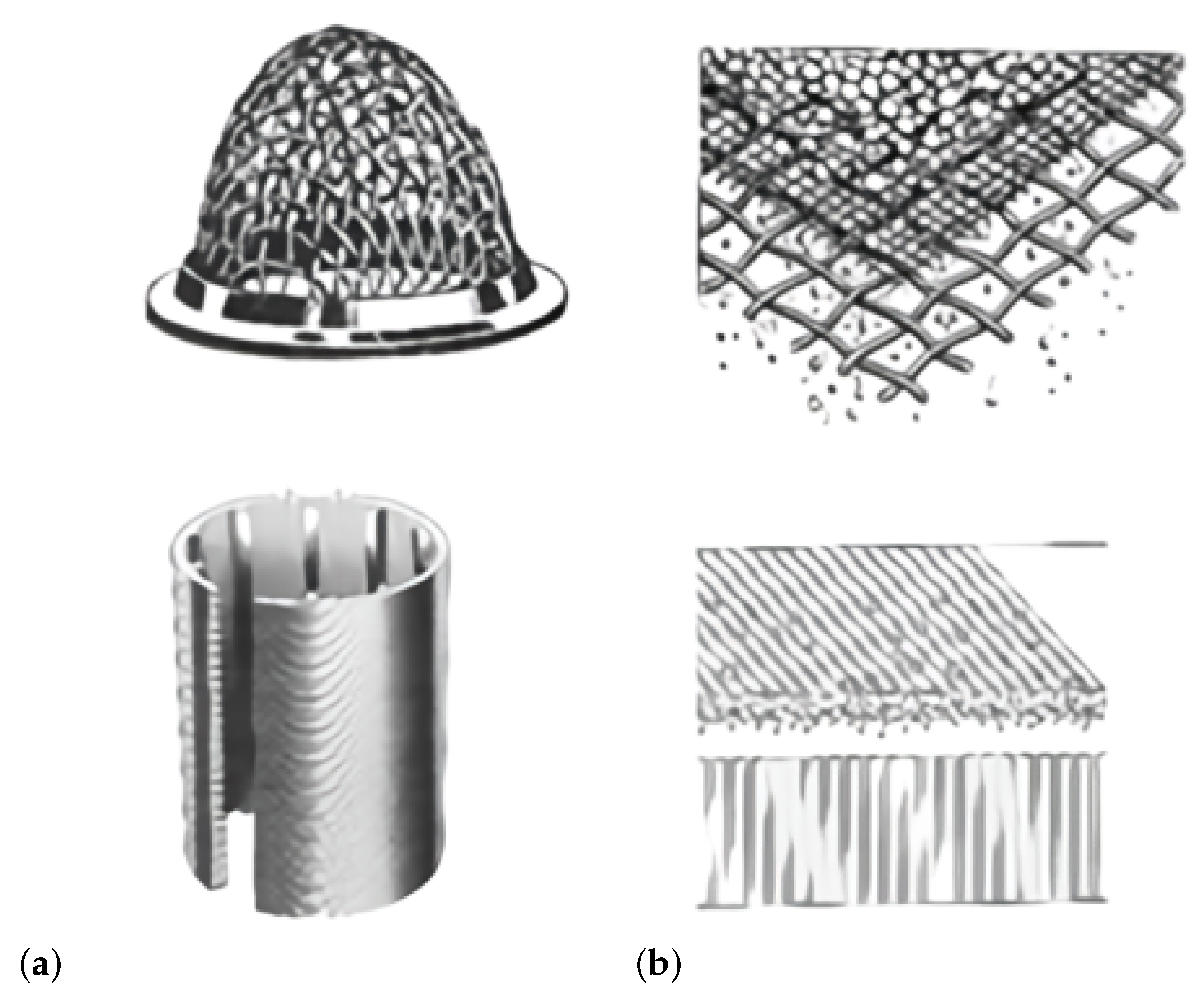
The screens that remove the debris entering an autostrainer have a circular wire shape and a wedged wire shape, as shown in Figure 4. The structure of the circular wire shape weaves circular wires like a net to determine the mesh count. The larger the number of meshes, the smaller the size of hole and the thinner the thickness of wire. For the performance of filtration, the net may be easily stretched or sag through the abrasion and pressure caused by fluids. A constant filtration effect can be obtained if the shape of the screen does not change during the operation from the mesh set at the time of design, but it is nearly impossible to obtain such an effect. In order to prevent these changes, it is mandatory to have a separate support. Debris included in the fluid may become stuck between wires, and this is not easy to clean. Regardless of the intention of the design, the thickness of the wire is determined according to the size of the mesh, and therefore it is difficult to respond to the pressure and shape of fluids. The structure of wedged wire maintains a constant gap between wires in an inverted triangle to wind up like the shape of a spring and maintain the gap with this support. The gap and size of wire can be determined by the pressure and flow of the passing fluid. When performing filtration, it is possible to filter debris included in the fluid by the size of the design, and the filtration proceeds from the wide surface to the narrow surface of the inverted triangle wires. In view of the progressive direction of the fluid, as the front surface of the filtration is wider than the rear surface, the possibility of blockage by debris is low. As the thickness gap of wires can be selected according to the type and pressure of fluid, this has the advantage of retaining a stable structure. In addition, this can be used semipermanently. Recently, this designed has been installed and used in most domestic water treatment plants.
Figure 5 shows the cross-section of the slot that composes the screen. In general, the standardized profile of the manufacturer is used. The slot used in the present study was the 18S Profile, which has the following dimensions: 1.5 mm width (b), 2.5 mm height (h), 12° angle (), and 2.4 mm cross-sectional area (Q). Fluid on the screen flows in the profile direction of the wide path from the profile of the narrow path. To remove debris between screens, the flow of backwashing proceeds in the opposite direction to the fluid path.
2.1.2. Design of Autostrainer Screens
The length of the screen is 200 mm in the region of passing water, where the autostrainer is installed. There are a total of 10 screens. Among those, 9 screens are used to remove debris and one screen is used for backwashing. Therefore, the total length of screen for filtration is The clearance between slots is 0.4 mm and the width of a slot is 1.5 mm. The penetration rate of water passing the screen is 0.2105, as shown in Equation (1). The area of screen can be obtained using Equation (2). This area can be expressed as an equation to obtain the linear velocity, as shown in Equation (3). Linear velocity means the velocity of water approaching the screen. As Equations (2) and (3) have the same value, if the amount of flow is 180 m/h in the end, the linear velocity of 0.6954 m/s can be obtained. From Equations (1)–(3), the size of the screen can be obtained for the design flow.
Applying the Equation (1), we obtain the calculation
Furthermore, using the Equation (2), we obtain
Using the result of Equation (1), 0.2105, the Equation (3) gives the screen surface area () value of
From this, we can see that v is 0.6954 m/s.
Here, ID refers to the inner diameter (m) of the screen, L is the length (m) of screen, capacity is the amount of inflow (/h), and is the approaching velocity (m/s).
2.1.3. Application of CFD to Autostrainers
In order to apply CFD to autostrainers, an analysis was implemented of the cross-section of screen slots, including the shape of the blockage. To apply CFD to the entire shape of the autostrainer, a porous model was applied for the region of the screen. Then, the coefficient of the resistance value for the porous model was derived from the result of CFD for the cross-section of the screen slots.
2.2. Shape Modeling and Grid System Construction for CFD Analysis
2.2.1. Shape Modeling and Grid System
- Application of CFD for the cross-section of the slot (2D shape)
In order to implement 2D CFD, as shown in Figure 6, a shape was assumed for the virtual blockage of the screen. The blockage rate was defined as in Equation (4). Figure 6a shows the assumption of the reduced region at the inlet in the flow direction after the generation of a blockage by debris from the front screen. Figure 6b shows the assumption of the reduced region of flow inlet after debris becomes stuck in front of the screen. Figure 6c shows the assumption of the generated blockage after debris becomes attached in the middle region of the slot. When performing the CFD for the 2D shape, we proceeded with a scenario which increased the blockage rate by 10% from 0% to 50%.
- Application of CFD to autostrainers (3D-shape)
In order to conduct the CFD for the inside of the autostrainer, as shown in Figure 7, modeling was carried out of its shape based on the diagram. The diameters of both the inlet and the outlet were 200 mm. A total of 10 screens were installed, numbered from No. 1 to No. 10. Screen No. 10 was for the backwashing, due to the blockage caused by debris. The length of the flow path on the screen was 200 mm. The thickness of the flow direction on the screen was applied with a slot thickness of 2.5 mm, to apply the resistance coefficient of the porous model. If modeling was performed for a real shape to create grids, the economies of computation would decline on account of the existence of many grids. Accordingly, the present study applied the porous mode. In addition, to achieve a more precise prediction of the inner fluid movement of the autostrainer, modeling was performed for the pipe on the backwashing side to conduct the study.
Figure 6.
Modeling of the 2D shape of the slot cross-section. (a) Scenario 1. (b) Scenario 2. (c) Scenario 3.
Figure 6.
Modeling of the 2D shape of the slot cross-section. (a) Scenario 1. (b) Scenario 2. (c) Scenario 3.
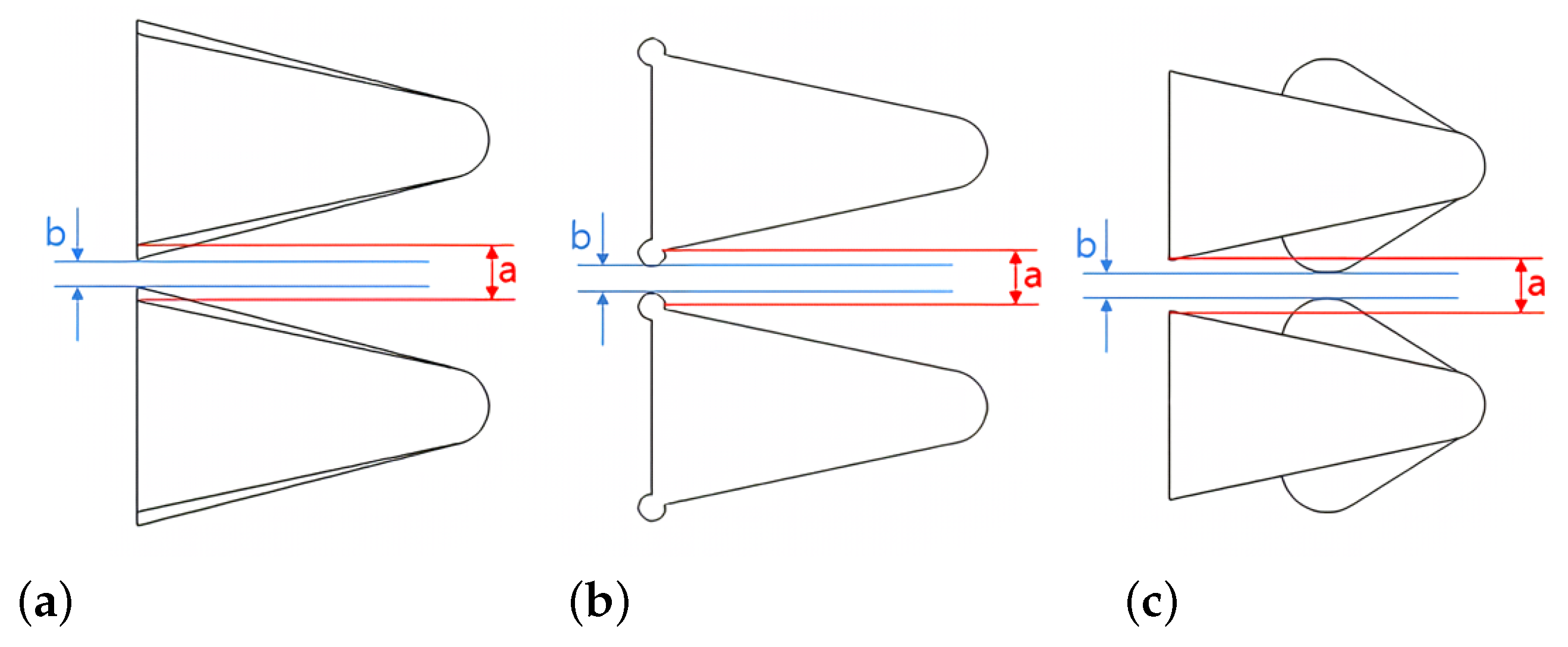
Figure 7.
Modeling of the autostrainer shape for CFD.

- Composition of the space grid system for CFD
In order to apply the said analysis, for the composition of the grid system, approximately 240,000 nodes were created per scenario for the 2D shape and applied to the system for calculation. For the 3D shape, approximately 1,320,000 nodes were applied. For the region that corresponded to the wall surfaces of the 2D shape and the 3D shape, the composition of a dense grid system was applied to improve the accuracy of calculation.
2.2.2. Numerical Approach
For the numerical analysis, the universal commercial code ANSYS CFX12 was employed. Typically, such universal commercial codes incorporate foundational algorithms like SIMPLE or SIMPLEC, as well as the Rhie and Chow method, which are primarily based on solving fluid flow problems involving pressure equations. These fundamental algorithms play a crucial role in accurately modeling the interactions between the pressure and velocity within fluid dynamics simulations. The codes that are based on these pressures provide various physical models and boundary conditions, which can be applied to problems of complex multi-physics that include the interconnection with other CAE tools. ANSYS CFX analyzes the equation obtained from the discretization through the full implicit pressure-based finite volume method using an algebraic multi-grid coupled solver. Compared to the segregated method of SIMPLE, the implicit coupling method accelerates the convergence and avoids the difficult point of convergence in pressurized flow. In addition, this technique is necessary because it handles grids with a high aspect ratio. In the numerical analysis of the application of a model for turbulent flow, some have claimed that a simple turbulent model provides sufficient accuracy, while others hold the opinion that the most developed turbulent flow model should be used to ensure the accuracy of analysis. The present study applied the turbulent flow model, which has been widely used commercially. In order to apply the porous model (2), the resistance coefficient is needed. In ANSYS CFX, permeability and loss coefficients as in Equation (5) and linear and quadratic resistance coefficients as in Equation (6) can be used. Equation (5) is applied when the density and viscosity are considered, which are composed of the velocity and pressure relations that express the permeability and the loss coefficient . In this study, Equation (5) was applied, considering density and viscosity, which expresses the permeability and loss coefficient in terms of the fluid’s velocity and pressure relationship. Here, ’U’ denotes the velocity of the fluid, referring to the average velocity as the fluid passes through a porous medium. The use of is a convention in fluid mechanics to represent velocity. The consistent use of this symbol throughout a document is important to clearly denote the velocity of the fluid. Specifically, plays a crucial role in the term related to laminar flow, and the term related to turbulent flow. The term is related to laminar flow and the term to turbulent flow. Equation (6) is applied to cases where the change in density and viscosity is ignored. and are obtained from the velocity and pressure relations and applied for calculation. As the present study corresponded to turbulent flow, was obtained and applied to the said analysis. In order to find the value of, , the resistance coefficient was calculated through an analysis based on the 2D scenario and its results. Its value was applied to the porous model of the 3D shape.
2.2.3. Boundary Condition for Numerical Analysis
For the boundary condition to apply numerical analysis, the flow condition was applied for the inlet and the pressure condition for the outlet, for each 2D scenario. A symmetry condition was applied for the top and bottom of five slots. For the turbulent flow model, its economy was considered when applying the widely used turbulent flow model and to derive the result of the pressure difference between the inlet and the outlet for each scenario. For the relations between this pressure difference and the inlet velocity, resistance coefficients were derived for each scenario of blockage to apply the porous model for 3D analysis. For 3D analysis, the mass flow rate (kg/s) was applied as the inlet boundary condition, the pressure condition as the outlet boundary condition, and the turbulence model, which is a commercially used turbulence model condition. In addition, a no-slip boundary condition was applied to the wall surface.
3. Experimental Results and Analysis by Scenario
3.1. Two-Dimensional Analysis Results for Each Scenario
Figure 8 shows the results of the velocity distribution from the results of the 2D analyses performed for each scenario. In Figure 8, (a) shows the velocity distribution that corresponds to a 0% blockage rate, (b) 50% blockage rate for scenario 1, (c) 50% blockage rate for scenario 2, and (d) 50% blockage rate for scenario 3. In the region where the flow path becomes narrow due to the gap of slots in the screen, fast velocity of fluid occurs, and the wide region shows the distribution of the slow velocity. Such a velocity difference causes the occurrence of a pressure difference between the inlet and the outlet in the analysis region.
Figure 9 shows the graph of the pressure drop caused by the change in inlet velocity, according to the blockage rate for each scenario. The horizontal axis in Figure 9a shows the velocity (0.27 m/s∼1.1 m/s) of the inlet, while the vertical axis shows the result of the pressure difference between the inlet and the outlet. When the blockage rate increased, the pressure drop increased. When the inlet velocity increased further, the pressure drop increased. With the 0% blockage rate, the pressure drop was about 0.1 kPa, with an inlet velocity of approximately 0.27 m/s. However, with an increased inlet velocity of 1.1 m/s, the pressure drop was above 10 kPa. For the 50% blockage rate, the pressure drop was about 0.4kPa, with an inlet velocity of approximately 0.27 m/s. However, with an increased inlet velocity of 1.1 m/s, the pressure drop was found to be above 50 kPa.
3.2. Comparison between the Test Results of Pressure Differences and the Results of CFD for Autostrainers
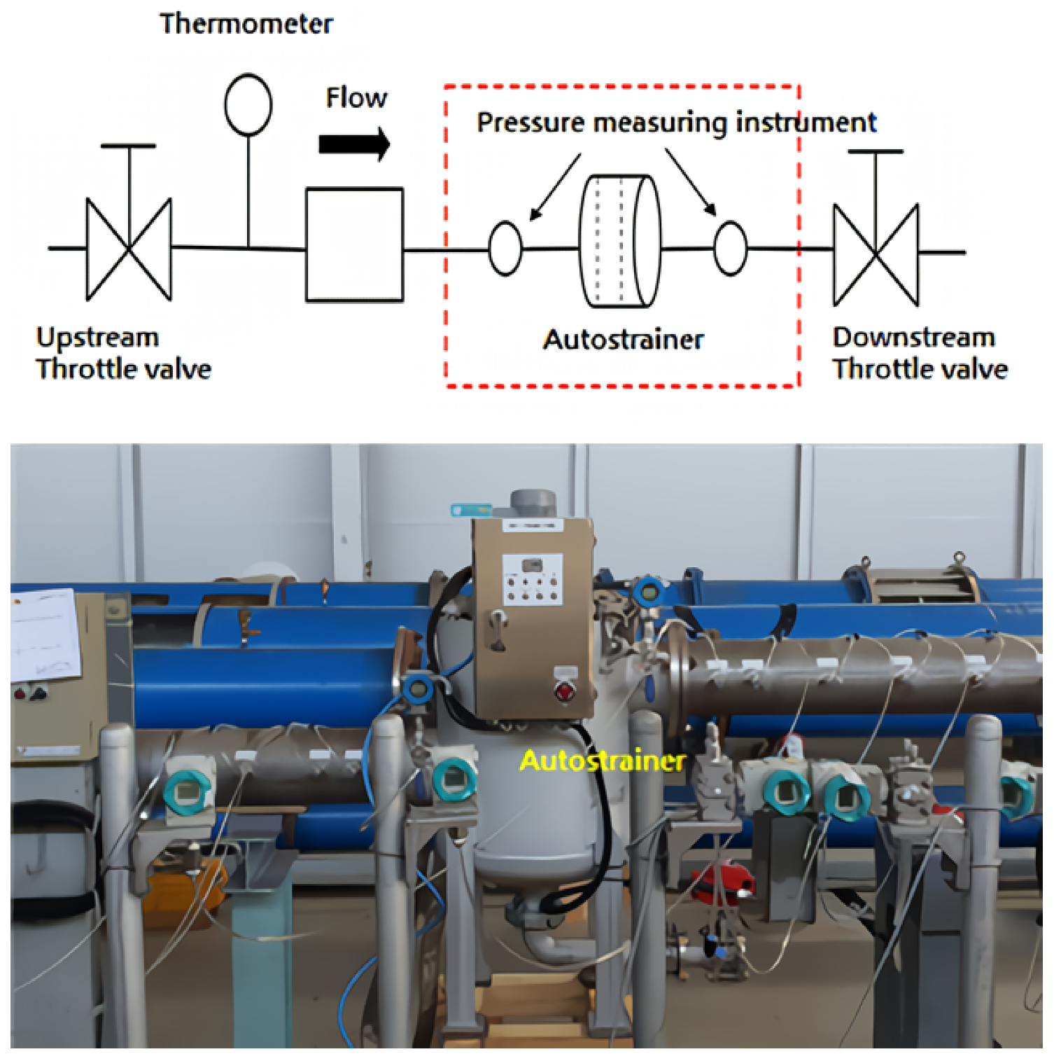
Tests were conducted to check the pressure difference caused by the change in flow in the autostrainer, which is the core element of the water intake system for the thermal source of deep water (source water) from a dam. Since a standard for the test on the autostrainer did not exist in South Korea, the test procedure for valve capacity (ANSI/ISA-75.02.01) was applied. Figure 10 shows the facility in which the pressure test of the autostrainer was performed. A valve and thermometer were placed upstream and a stroll valve was placed downstream to control the flow. In the test section, a total of 10 pressure taps were installed at the front end (0.5D = 100 mm, 1D, 2D) and the rear end (0.5D, 1D, 2D, 3D, 4D, 5D, 6D) to check pressure changes for testing.
Figure 11 shows the comparison between the test values of the autostrainer and the results of CFD for the 3D shape. The graph shows the pressure difference and headloss coefficient of the flow change. Figure 11a shows that a lower result was obtained from the application of the porous resistance coefficient derived from the analysis result of CFD for the 2D shape compared to the test value of the pressure difference for the flow change. When the corrected porous resistance coefficient was applied, a similar result for the pressure difference was derived as for the test value. As seen in Figure 11b, the headloss coefficient of the flow change had a 3.78% difference between the maximum value and the minimum value, and the average value was approximately 5.2. Upon application of the porous resistance coefficient, which had been derived from the analysis result of CFD for the 2D shape, the difference between the maximum value and the minimum values was 1.9%. The headloss coefficient had an average of 4.9. When the corrected resistance coefficient was applied, the difference between the maximum value and the minimum value was 0.3%. The headloss coefficient had an average of approximately 5.2, which was similar to the test value. Later, for the application to CFD of the 3D shape, the corrected resistance coefficient was applied to derive the headloss coefficient.
3.3. Analysis Results of 3D CFD According to the Screen Blockage Rate
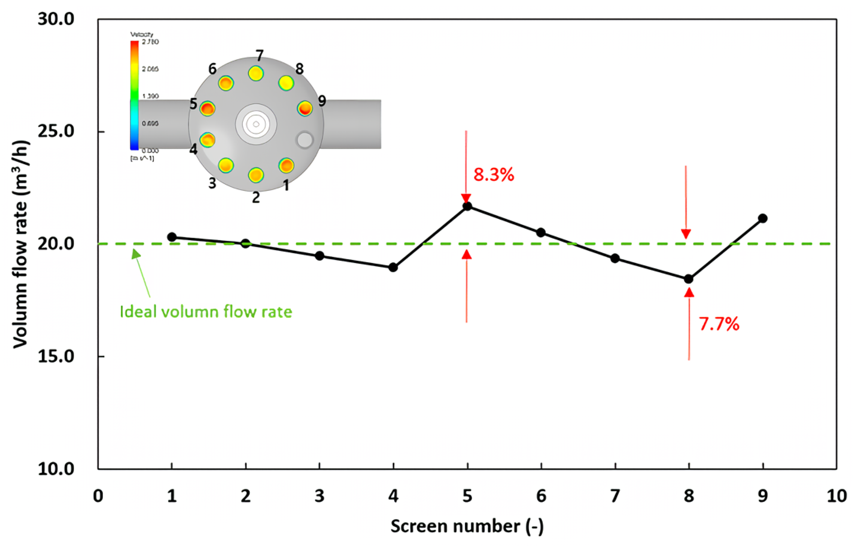
Figure 12 shows the amount of inflow to each screen at a flow velocity of 180 m/h. The ideal amount of inflow to the screen was 20 m/h for uniform inflow. According to the characteristic of inner flow, the amount of inflow to the screen will not be uniform. Fluid flows from the inlet to the screen to the outlet, and the resistance to flow through each screen is different. This results in a change in flow rate as the pressure changes due to the different resistance of each screen as the fluid passes through screens 1 to 9. The ideal flow rate is 20 m/h, but due to the pressure difference between each screen, the flow rate decreased in areas with large pressure losses 1–4 and increased by 8.3% in area 5 with small pressure losses. Up to screen No. 8, the amount of inflow decreased again. At screen No. 8, an inflow that was 7.7% lower than the average entered the screen. At screen No. 9, an inflow that was higher than the average inflow entered the screen. Based on such results, we could predict that in the region where a relatively low amount of inflow occurs, a high blockage rate of screen will occur. In addition, the inflow velocity in the vertical direction of the screen is one of the most important elements that is applied to the blockage rate of a screen. This means that the blockage rate of the screen shows different values in the vertical direction. Figure 13 shows that the inflow velocity on the top was lower than the inflow velocity at the bottom. As the velocity on the top of the screen was relatively lower, in the top region of the screen, a high blockage rate value was predicted to appear.
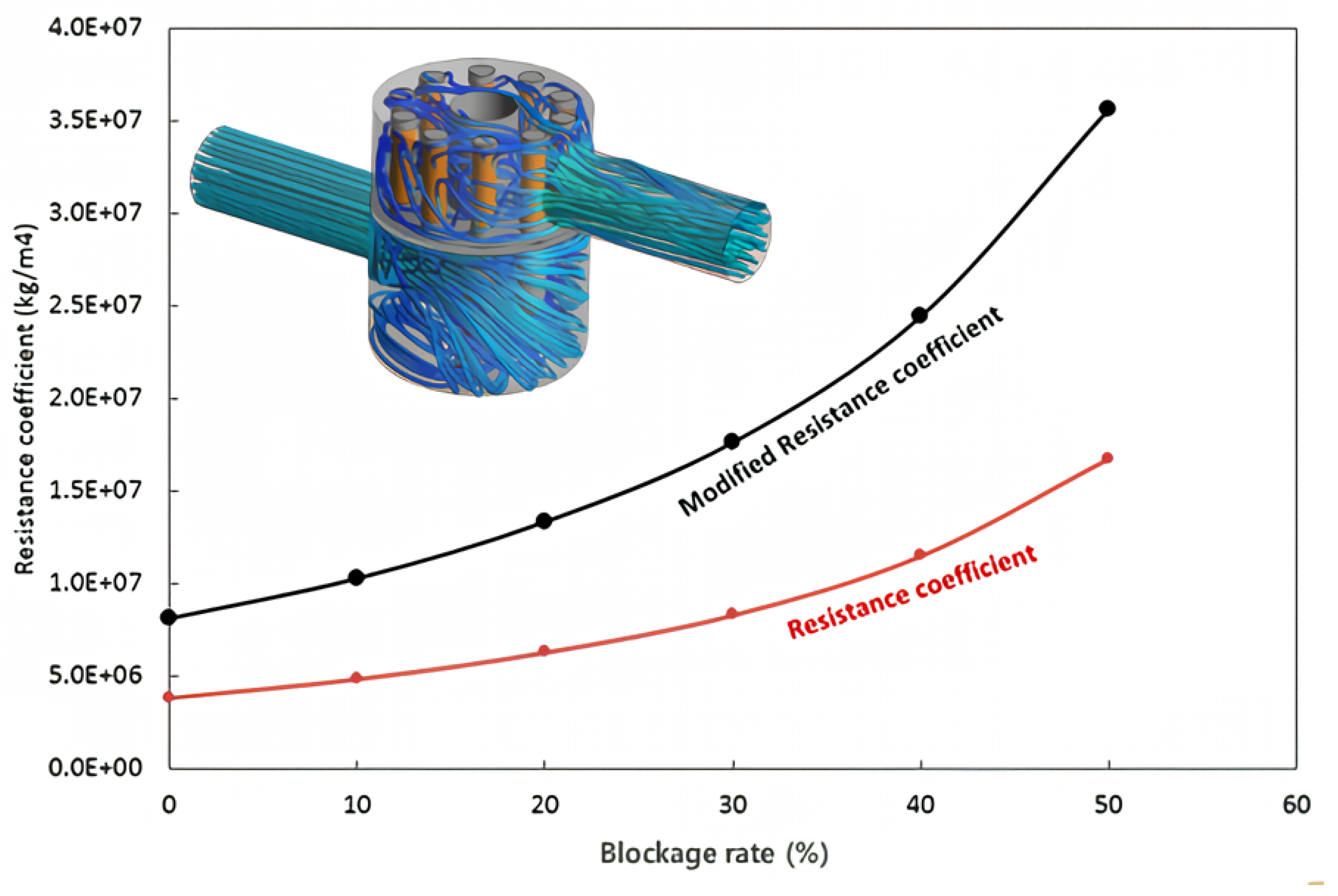
In the 2D analysis, the results of the coefficient values to be applied to the 3D porous domain were derived for each scenario’s occlusion rate shape, and the coefficient values of each occlusion rate derived in 2D were applied to the 3D shape for analysis. In order to apply 3D CFD according to the blockage rate of the screen, the value of the porous resistance coefficient was needed. The red graph in Figure 14 shows the porous resistance coefficient derived from the CFD results of the 2D shape. When the resistance coefficient was quantitatively used for the 0% blockage rate, it had a lower value than that of the test result. As the value of the test result appeared similar to the application of the corrected blockage rate for a 0% blockage rate, based on this resistance coefficient, the value of the resistance coefficient derived from the 2D result was obtained according to the blockage rate, expressed in black. Later, this value was applied to derive the CFD result according to the 3D blockage rate.
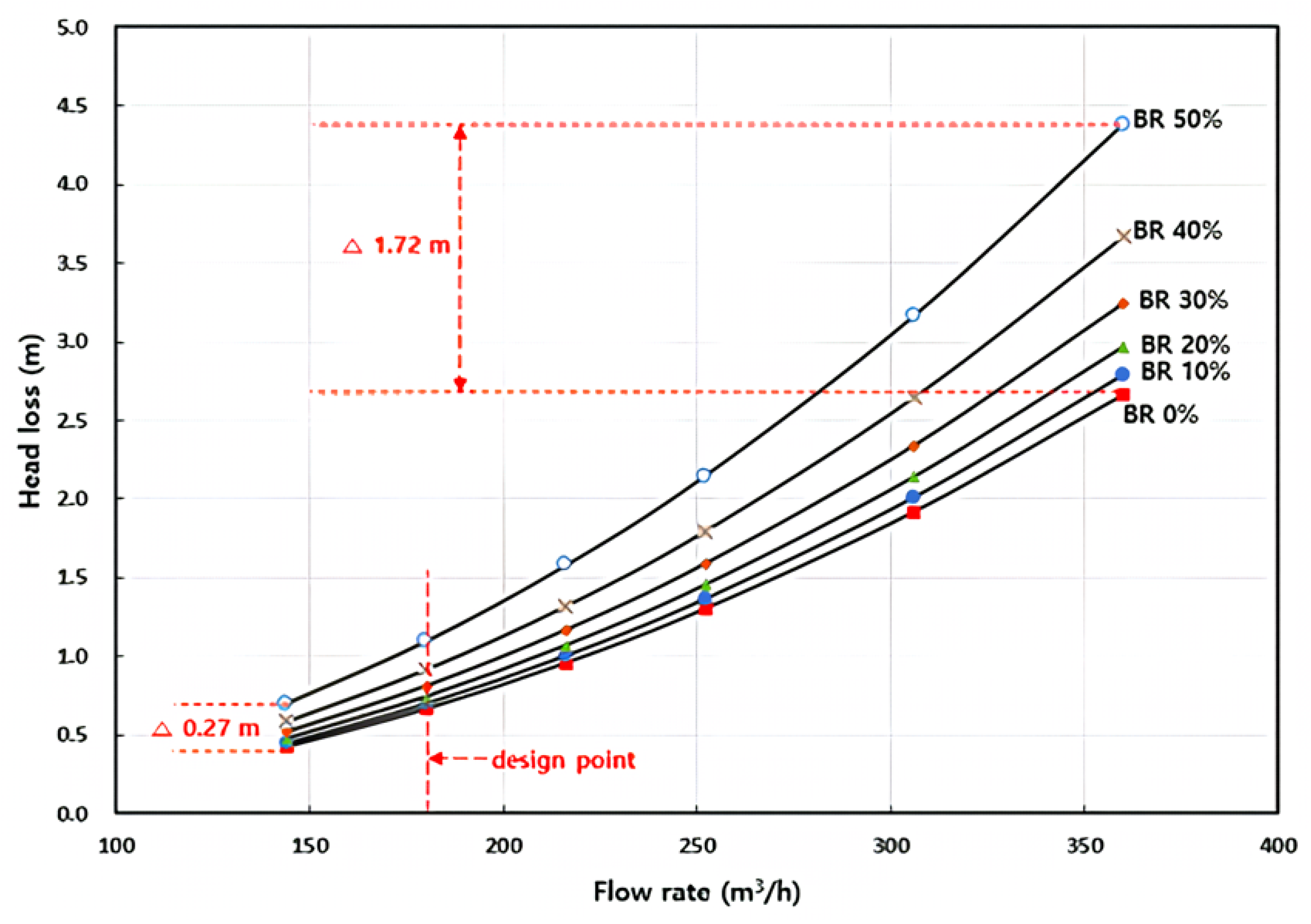
Figure 15 shows the headloss of the flow change through the application of the same blockage rate to the screens. The design flow was 180 m/h. The headloss was found to be 0.27 m with the increase in the blockage rate from 0% to 50%, which corresponds to 80% of the flow. When the flow was increased by 200%, the difference in headloss between 0% and 50% was found to be 1.72 m. The headloss with 80% flow was 0.75 m for the 50% blockage rate of screens. This value shows that the headloss increased to about 4.4 m when the flow increased by 200%. As the flow increased and the blockage rate of the screens increased, the headloss increased.
During the actual operation of the autostrainer, the blockage rate of the screens was predicted to show little difference locally. As an example of obtaining the headloss caused by such a phenomenon, the blockage rate was applied differently in the vertical direction of the screen to implement CFD. Figure 16 shows the results. From the previous result of the velocity distribution for the inflow to the screen, as the velocity of the inflow to the top was lower than that to the bottom, the blockage rate applied was higher at the top than at the bottom. As the flow increased, the headloss showed a significantly large change. As the blockage rate became higher, its slope, which indicates the amount of change, became much larger.
4. Discussion—Design Parameters
4.1. Headloss Coefficient (K), Flow Coefficient (Cv), Discharge Coefficient (Cd)
It is possible to select a pump and a heat exchanger when the resistance value of the system is derived in the design of the water intake system. In order to derive the resistance value of the system, the design parameter of headloss value (K) is mainly utilized, which is defined as in Equation (7).
Here, refers to the headloss (m), g is the acceleration of gravity (m/s2), and v is velocity (m/s).
The design parameter used much for the valve is the flow coefficient, which is defined as in Equation (8).
Here, Q is the volume flow (m/h), G is the specific gravity (water = 1), and is the pressure difference (bar).
In flow limiting devices, such as nozzles or orifices, the discharge coefficient is used: this coefficient expresses the rate of actual flow and theoretical flow, which is defined as in Equation (9). Theoretical flow is the flow without loss, for which we can apply Bernoulli’s theorem. As there is a pressure loss in actual flow, the actual flow is smaller than the theoretical flow and the discharge coefficient will be smaller than 1 (a value closer to 1 indicates less pressure loss).
Here, is the actual flow, is the theoretical flow, is the mass flow (kg/s), A is the cross-sectional area of flow path (m), is the density (kg/m), and is the pressure difference (Pa).
Table 1 shows the coefficient value results obtained when the same blockage rate was applied to the screen. As the blockage rate increased, the headloss coefficient (K) increased, while the flow coefficient (Cv) and the discharge coefficient (Cd) decreased. Table 2 shows the headloss coefficient, the flow coefficient, and the discharge coefficient when the local blockage rate was applied in the vertical direction of the screens. Figure 17 shows these results in a graph of the headloss coefficient and the discharge co-efficient. With the local blockage rate from 40% to 50%, a relatively large slope occurred. We can thereby conclude that it is economically advantageous to implement backwashing in this region.
4.2. Additional Consideration (Particle Settling Rate)
Stoke defined the settling velocity of particles as shown in Equation (10) when particles are dropped in a region without any flow (Figure 18).
Here, g is the acceleration of gravity (m/s), d the size of particle (m), the viscosity coefficient of water (m/s), the density of particle (kg/m), and the density of water (kg/m).
If the increasing fluid velocity is greater than the settling velocity of the particle, the settling rate will be 0%. From the analysis results at an inlet flow of 180 m/h in the autostrainer, the average increasing velocity of flow was found to be 0.00458 m/s. When this value is applied to the theoretical settling velocity of Stokes, as shown in Figure 19, the settling region will appear for the size and density of particles. However, as the characteristic of inner flow in the autostrainer has a complex structure, a separate analysis was necessary for the diameter and density of each particle. Sediment build-up interferes with the backwashing process, causing headloss. Figure 19 shows how much of an impact sediment can have.
Figure 20 shows the results obtained to verify the amount of settling with the change in the size and density of particles, assuming the debris to be particles in the inlet of the autostrainer. In the application of CFD, it was assumed that particles had a spherical shape. It was assumed that mutual interaction between particles, such as collision, collapse, and coalescence between particles, would not occur. When the smallest size of the inflow particle was 1 m, the settling rate was approximately 3%. With the same density, as the diameter of the particle increased, the settling rate increased with the increased mass of the particle. In addition, with the same size of particles, when the density increased, the settling rate of particles increased. For example, the density of sand was 2640 kg/m. The graph with the density of 2500 kg/m shows that if the diameter of particle was 300 m, the settling rate increased to 35%. Here, if the diameter of particles was 400 m, the gap between the slots of the screen was 400 m, and therefore a diameter larger than this was filtered by the screen. It is considered such that settling will occur according to the characteristic of the debris that enters from the inlet of the autostrainer. A structure must be included to discharge such sediments, namely sludge, out of the strainer.
5. Conclusions
The values of pressure loss were obtained according to the blockage rate of the screen in an autostrainer utilizing CFD. With these values, the design parameter of the headloss co-efficient (K) was derived. The values of the headloss coefficient were derived to be 5.150, 5.393, 5.752, 6.267, 7.097, and 8.497 in cases where the blockage rates were 0%, 10%, 20%, 30%, 40%, and 50%, respectively. The headloss coefficients in the application of the local blockage rate were derived to be 5.223, 5.515, 5.940, 6.587, and 7.651 in cases where the blockage rates were 0–10%, 10–20%, 20–30%, 30–40%, and 40–50%, respectively. These values can be utilized to obtain the resistance value of the system to select the pump and the heat exchanger. The headloss coefficient (K) values obtained in this study can be utilized as an important indicator to measure the pressure loss due to the screen clogging rate of the autostrainer. These values help to determine the resistance value of the system for selecting pumps and heat exchangers. Furthermore, these values based on the clogging rate can be useful to investigate the applicability of membrane filtration based on the clogging rate. By considering key variables such as settling rate and resistance values, it is expected to help design an appropriate water intake system to achieve optimal operating efficiency.
Author Contributions
I.M. performed the data analysis and discussed the results, J.C. and G.K. performed the measurements and simulations. H.J. performed the numerical calculations. We discussed the results and wrote the manuscript with input from all co-authors. All authors have read and agreed to the published version of the manuscript.
Funding
Open access funding was enabled and organized by the Ministry of Environment (Task Serial Number: 2020003130001).
Data Availability Statement
Data is contained within the article.
Acknowledgments
The present study was conducted with support through the project for the development of environmental technology by the Korea Environmental Industry & Technology Institute, from the budget of the Ministry of Environment (Task Serial Number: 2020003130001).
Conflicts of Interest
The authors declare no conflicts of interest.
References
- ANSYS CFX-12.0 User Manual. 2012. Available online: https://www.afs.enea.it/project/neptunius/docs/fluent/html/ug/main_pre.htm (accessed on 11 April 2024).
- Lim, J.I.; Park, J.H.; Kim, J.H.; Kim, D.J. Flow analysis of sea-water strainer. Ksfm J. Fluid Mach. 2009, 333–334. [Google Scholar]
- Jung, I.S. A Study on Pressure Drop Analysis of Strainer for Vessels. Master’s Thesis, Dong-A University, Busan, Republic of Korea, 2012. [Google Scholar]
- Sin, B.G. An Experimental Study on the Design, Production and Performance Test of C-type Strainer for the Improvement of Flow Characteristics—With a Focus on the Comparison with Y-type Strainer. Ph.D. Thesis, Hanse University, Groningen, The Netherlands, 2016. [Google Scholar]
- Jameson, A.; Schmidt, W.; Turkel, E. Numerical Solutions of the Euler Equation by Finite Volume Methods Using Runge-Kutta Time Stepping Schemes. In Proceedings of the 14th Fluid and Plasma Dynamics Conference, Palo Alto, CA, USA, 23–25 June 1981. [Google Scholar]
- Denton, J.D.; Xu, L. The Effects of Lean and Sweep on Transonic Fan Performance. In Proceedings of the ASME Turbo Expo 2002: Power for Land, Sea, and Air, Amsterdam, The Netherlands, 3–6 June 2002. [Google Scholar]
- Lee, Y.G.; Yuk, J.H.; Kang, M.H. Flow Analysis of Fluid Machinery using CFX Pres-sure-Based Coupled and Various Turbulence model. Ksfm J. Fluid Mach. 2004, 7, 82–90. [Google Scholar] [CrossRef]
Figure 1.
Reduction in efficiency with tip clearance.
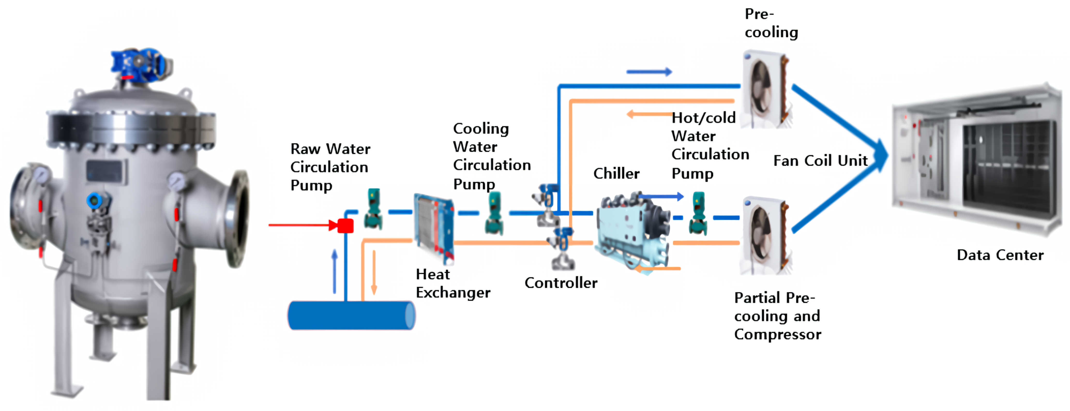
Figure 2.
Change in occlusion rate due to foreign debris introduction. (a) before (b) after.
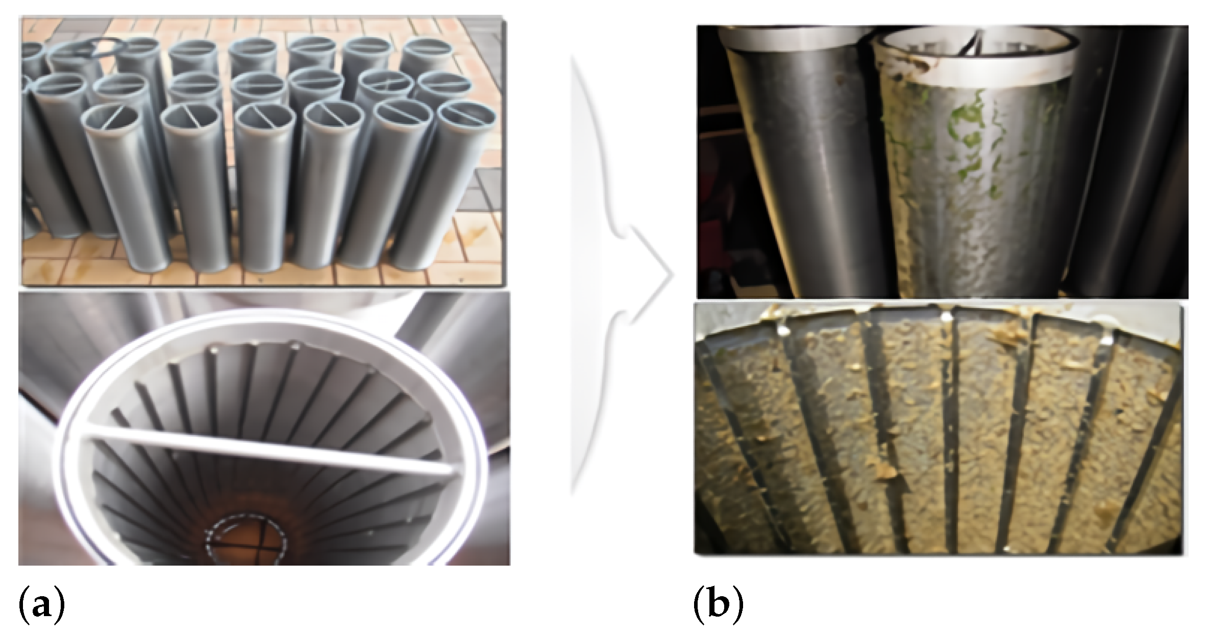
Figure 3.
Working and backwashing structure of the autostrainer.
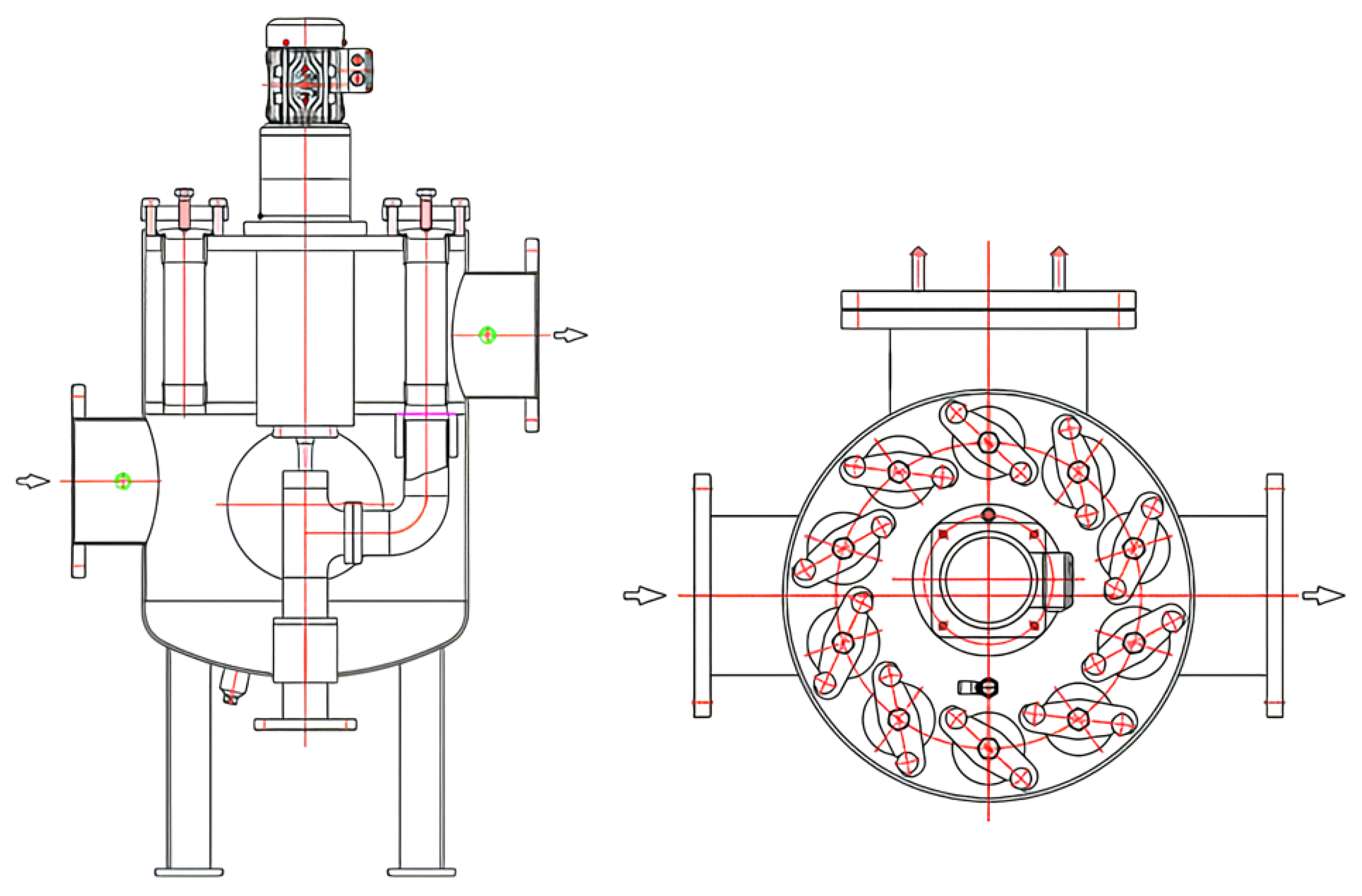
Figure 4.
Wire-shaped screen to remove entering debris. (a) Circle wire. (b) Wedged wire.

Figure 5.
Cross-section of the slots that make up the screen.

Figure 8.
Two-Dimensional Analysis Results for Each Scenario. (a) Blockage rate 0%. (b) Scenario 1—Blockage rate 50%. (c) Scenario 2—Blockage rate 50%. (d) Scenario 3—Blockage rate 50%.
Figure 8.
Two-Dimensional Analysis Results for Each Scenario. (a) Blockage rate 0%. (b) Scenario 1—Blockage rate 50%. (c) Scenario 2—Blockage rate 50%. (d) Scenario 3—Blockage rate 50%.

Figure 9.
Pressure drop (2D) according to inlet velocity conditions. (a) Scenario 1. (b) Scenario 2. (c) Scenario 3.
Figure 9.
Pressure drop (2D) according to inlet velocity conditions. (a) Scenario 1. (b) Scenario 2. (c) Scenario 3.
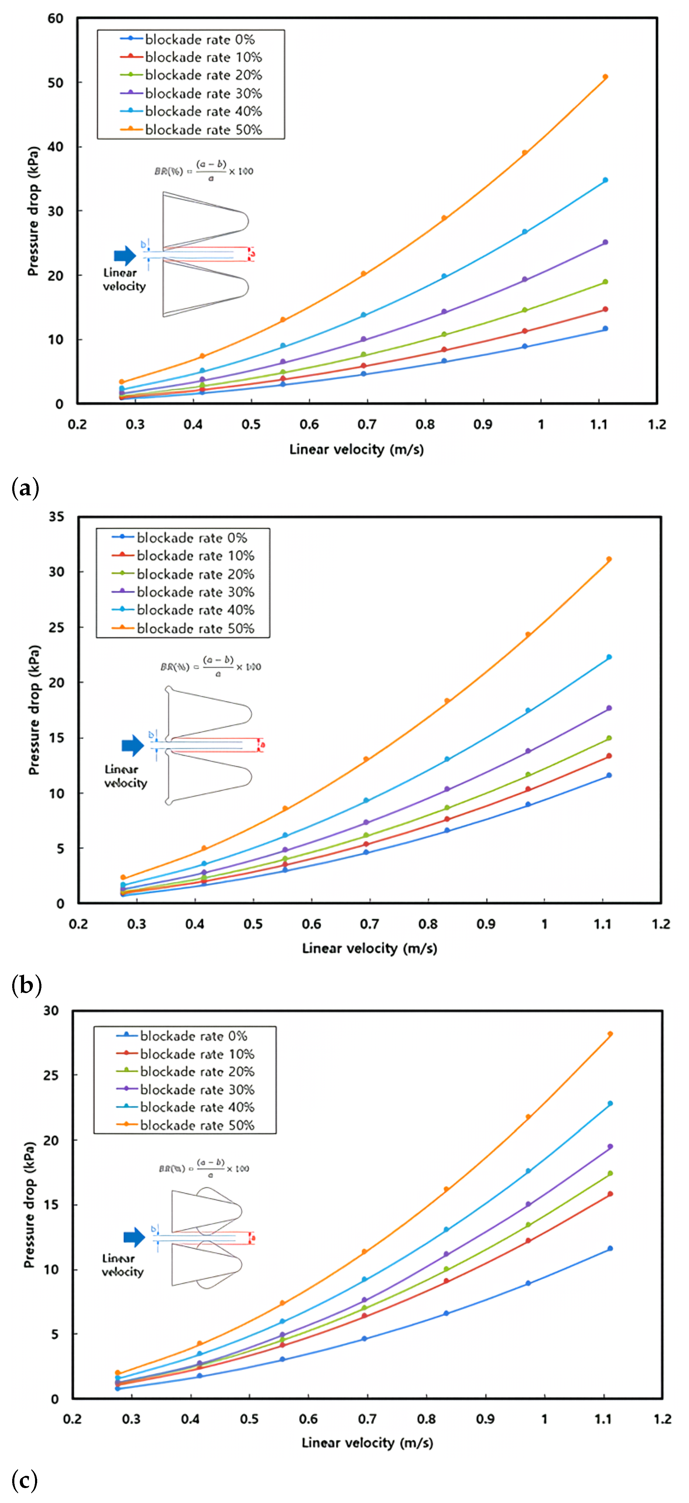
Figure 10.
Pressure test of the autostrainer.

Figure 11.
Results of the experiment and CFD. (a) Differential in-out pressure. (b) Headloss coefficient.
Figure 11.
Results of the experiment and CFD. (a) Differential in-out pressure. (b) Headloss coefficient.
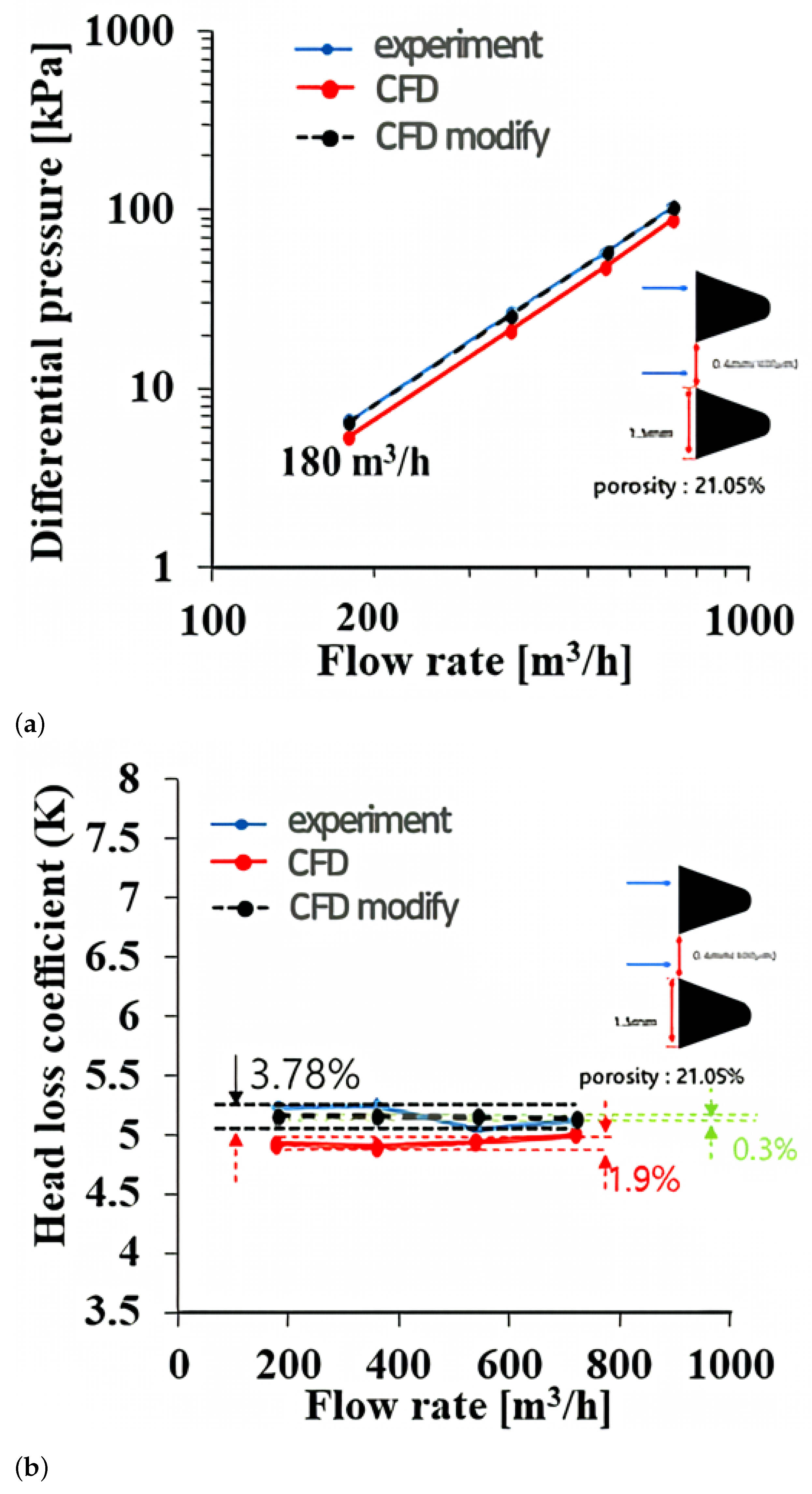
Figure 12.
Comparison of the amount of inflow to the screen in the screen blockage rate %.

Figure 13.
Velocity distribution in the vertical direction of the screen in blockage rate %.

Figure 14.
Porous resistance coefficient using the screen blockage rate.

Figure 15.
Headloss in the application of the blockage rate to screens.

Figure 16.
Headloss in the local application of the blockage rate to screens.
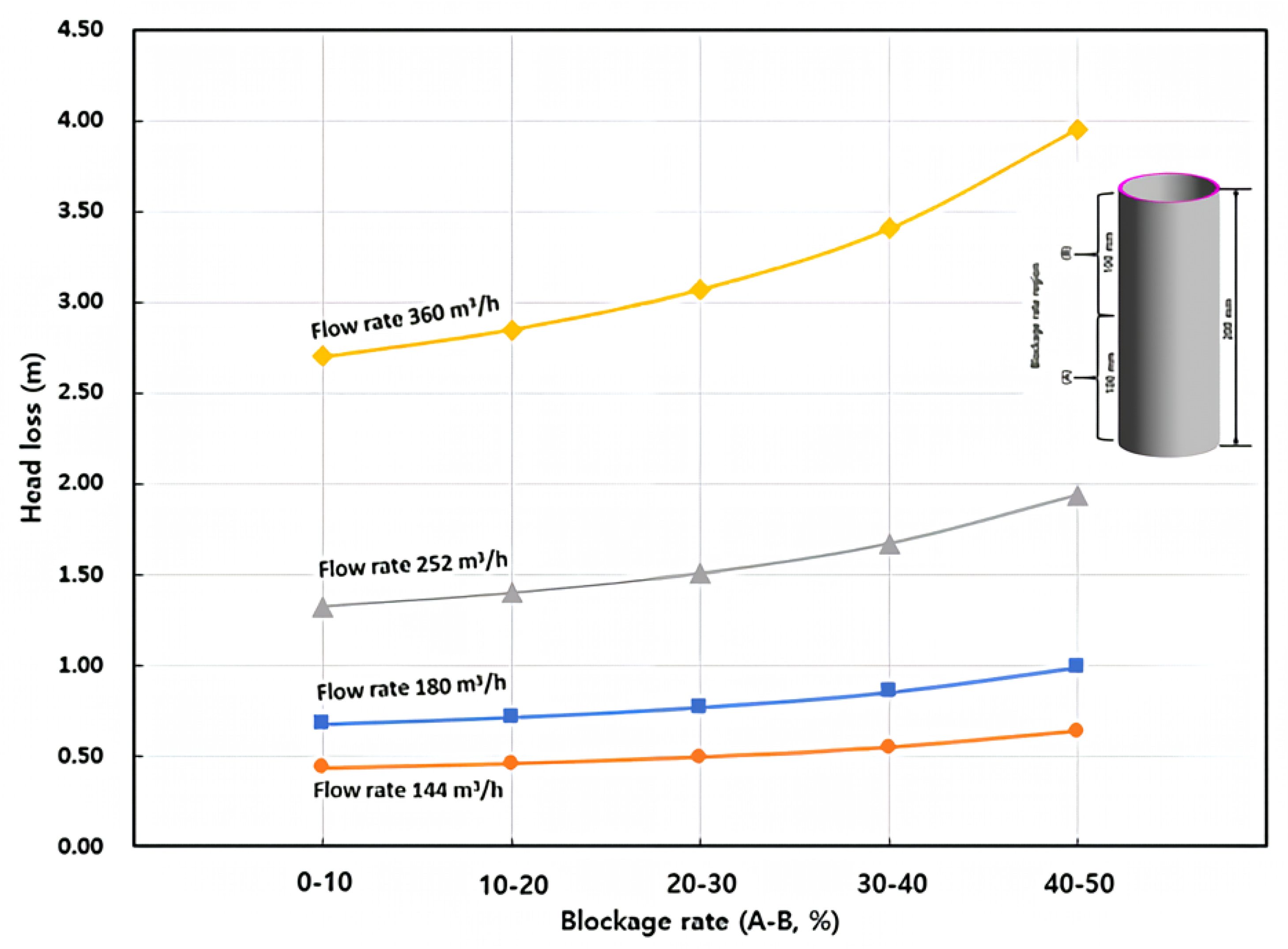
Figure 17.
Coefficients of headloss and discharge of the application of the local blockage rate to the screen.
Figure 17.
Coefficients of headloss and discharge of the application of the local blockage rate to the screen.
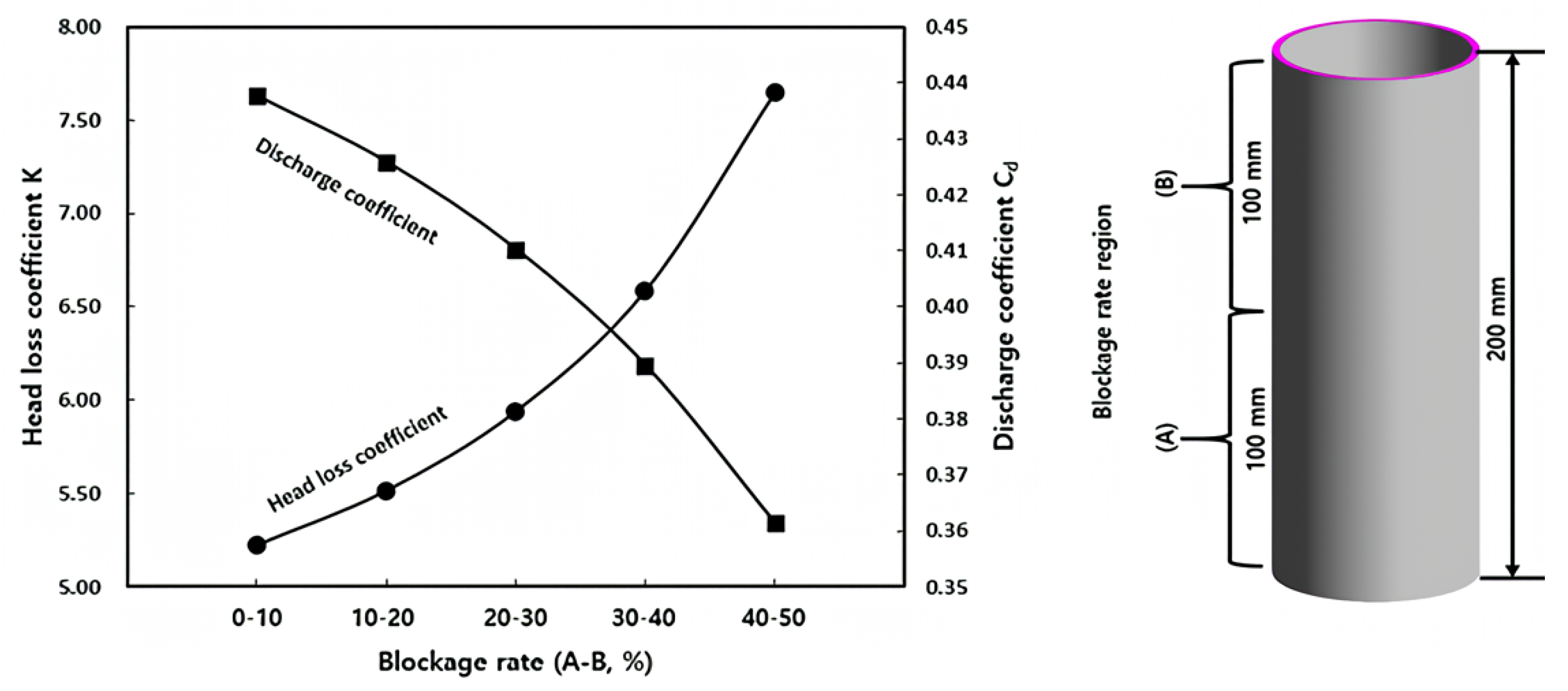
Figure 18.
Settling velocity of a particle inside a fluid without flow.
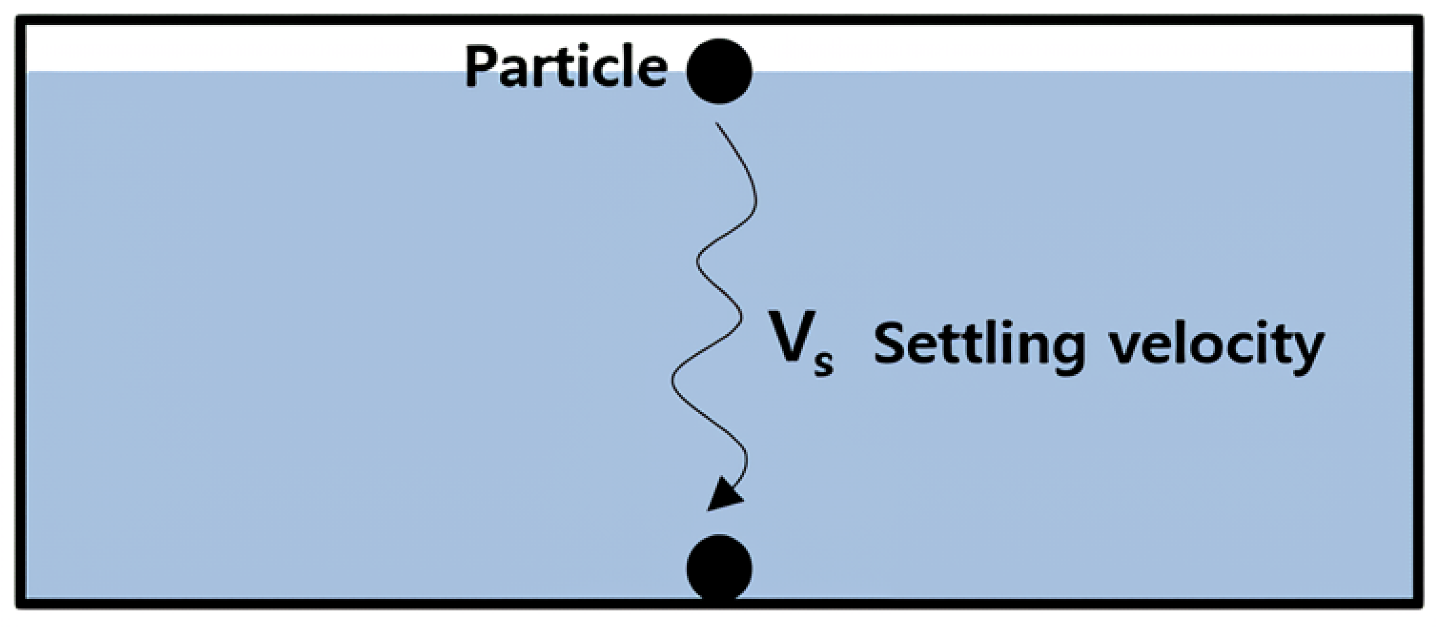
Figure 19.
Settling range of theoretical particles.
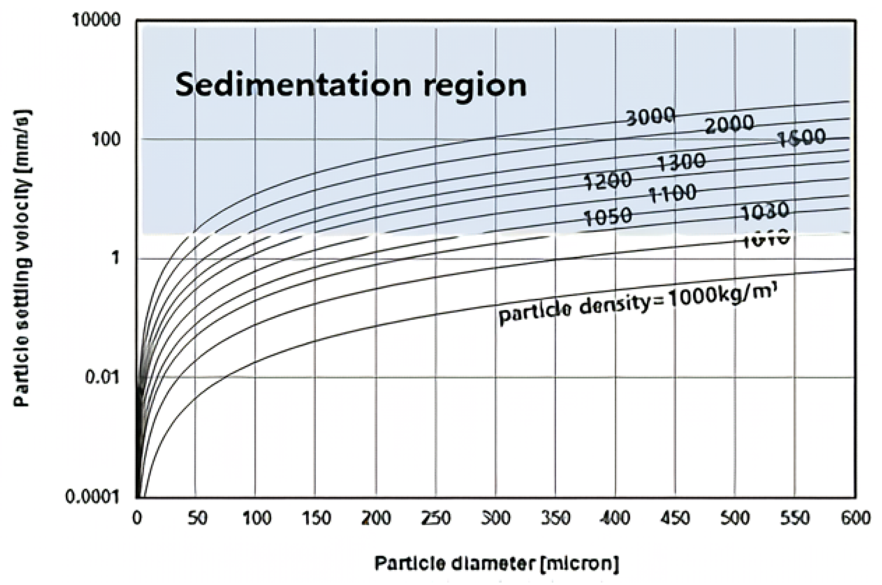
Figure 20.
Settling rate by the size and density of particles.


Table 1.
Coefficient values of the blockage rate to the screen.
| Blockage Rate (%) | Headloss Coefficient (K) | Flow Coefficient (Cv) | Discharge Coefficient (Cd) |
|---|---|---|---|
| 0 | 5.150 | 816.055 | 0.441 |
| 10 | 5.395 | 797.258 | 0.431 |
| 20 | 5.752 | 772.161 | 0.417 |
| 30 | 6.267 | 739.745 | 0.399 |
| 40 | 7.097 | 695.109 | 0.375 |
| 50 | 8.479 | 635.952 | 0.343 |
Table 2.
Coefficient values of the local blockage rate to the screen.
| Blockage Rate (%) | Headloss Coefficient (K) | Flow Coefficient (Cv) | Discharge Coefficient (Cd) |
|---|---|---|---|
| 0–10 | 5.223 | 810.296 | 0.438 |
| 10–20 | 5.515 | 788.583 | 0.426 |
| 20–30 | 5.940 | 759.830 | 0.410 |
| 30–40 | 6.587 | 721.519 | 0.390 |
| 40–50 | 7.651 | 669.486 | 0.32 |
Disclaimer/Publisher’s Note: The statements, opinions and data contained in all publications are solely those of the individual author(s) and contributor(s) and not of MDPI and/or the editor(s). MDPI and/or the editor(s) disclaim responsibility for any injury to people or property resulting from any ideas, methods, instructions or products referred to in the content. |
© 2024 by the authors. Licensee MDPI, Basel, Switzerland. This article is an open access article distributed under the terms and conditions of the Creative Commons Attribution (CC BY) license (https://creativecommons.org/licenses/by/4.0/).
Share and Cite
MDPI and ACS Style
Min, I.; Choi, J.; Kim, G.; Jo, H. CFD Analysis of the Pressure Drop Caused by the Screen Blockage Rate in a Membrane Strainer. Processes 2024, 12, 831. https://doi.org/10.3390/pr12040831
AMA Style
Min I, Choi J, Kim G, Jo H. CFD Analysis of the Pressure Drop Caused by the Screen Blockage Rate in a Membrane Strainer. Processes. 2024; 12(4):831. https://doi.org/10.3390/pr12040831
Chicago/Turabian StyleMin, Inhong, Jongwoong Choi, Gwangjae Kim, and Hyunsik Jo. 2024. "CFD Analysis of the Pressure Drop Caused by the Screen Blockage Rate in a Membrane Strainer" Processes 12, no. 4: 831. https://doi.org/10.3390/pr12040831
Note that from the first issue of 2016, this journal uses article numbers instead of page numbers. See further details here.