Low-Carbon Optimal Configuration of Integrated Electricity and Natural Gas Energy System with Life-Cycle Carbon Emission

Abstract

In response to the challenges of global warming and the development of A low-carbon economy, the integrated electricity and natural gas energy system (IEGES) is known as an important structure for future energy supply; thus, its planning and design must take low-carbon and environmental protection factors into account. Regarding carbon emissions as an optimization criterion, this paper built life-cycle carbon emission models of IEGES components. Then, taking the capacities of the energy resources, storage and conversion units of IEGES as the optimization variables, a multi-objective optimization configuration model was established considering the annual investment operation cost and the life-cycle carbon emissions. The multi-objective model was transformed into a single-objective one by an ε-constraint approach and the polynomial fitting method was employed to obtain the value of ε for obtaining uniformly distributed Pareto sets. Based on the fuzzy entropy weight method and the fuzzy affiliation degree approach, the obtained Pareto sets were ranked and the solution with the highest ranking value was selected as the optimal solution for the original problem. Finally, the configuration schemes were analyzed from the perspectives of economy, carbon emission and renewable energy utilization, and the effectiveness and rationality of the proposed optimization method were verified through MATLAB simulation.

1. Introduction

In recent years, with the growing prominence of environmental issues, realizing the decarbonization of energy production and utilization has become an inevitable trend for the sustainable development of human society [1]. To cope with the challenges of energy supply and demand conflicts and global warming, building a carbon-neutral energy system has become a consensus among countries around the world [2,3], and China has also put forward the strategic goals of “double carbon” and “new power system” [4]. An integrated energy system (IES) possesses the advantages of multiple energy complementarity and cascading energy utilization [5], which can effectively improve the energy utilization efficiency, promote the consumption of renewable energy power generation and reduce the energy cost for users. Moreover, many IES demonstration projects have confirmed the safety and reliability of IES and its potential for energy saving and emission reduction [6].

Currently, numerous studies on IES have been carried out in terms of the quantification of multi-energy resources [7,8], planning and operation optimization [9,10,11] as well as the comprehensive evaluation of energy systems [12]. Regarding the modeling of multi-energy resources, the coupling model between the energy supply system and the oil and gas production system is proposed in [13], and a reliability model of IES considering multi-energy correlation is established in [14], which presents a novel analytical method to model the dependent multi-energy capacity outage states and their joint outage probabilities for its reliability assessment. Moreover, a flexibility evaluation method considering the impact of multi-energy coupling is proposed in [15], which provides support for making full use of flexible resources and improving the operational economy. In terms of the planning of the IES, an optimal expansion planning model for an integrated energy system consisting of a power grid, a gas network and multiple energy hubs is proposed in [16], and the optimal configuration model of multitype energy storage for IES considering the system reserve value is built in [17], which can reduce the annual investment cost and operating cost and improve the system reserve capacity. Moreover, the optimal planning methods of IES with uncertainties are presented in [18,19], which consider the uncertainties of renewable energy and electricity prices. For the operation optimization of the IES, many objectives are utilized for IES optimization, such as the total operation cost, the revenue and the carbon emissions. For example, the operation cost and revenue are considered in [20] to achieve the optimal operation between different entities in the IES, and the operation cost and carbon emissions are included in [21] for obtaining the optimal design method of an integrated energy system under a low-carbon background. In addition to the operation cost, the environment cost model is proposed in [22], which consists of the environmental loss caused by the pollutants of energy generation and the resulting non-environmental loss. The above literature provides valuable insights for further research on IES.

In the low-carbon transition context, the planning of IES should not only consider the coupling of multiple energy resources, but also take the carbon emissions into consideration. The existing studies are mainly divided into two parts: one idea is to take carbon emissions as constraints of the IES planning model [23]; another idea is to incorporate carbon emissions into the objective function [24,25,26]. Specifically, in [23], the carbon peak, carbon neutrality and carbon quota constraints were introduced in the multi-stage planning model of an IES. The carbon emission benefits and environmental costs are introduced into the optimization objectives of the IES planning model in [26].

Inspired by the existing research, this paper focuses on the low-carbon planning problem of the integrated electricity and natural gas energy system (IEGES). Based on the whole life-cycle analysis method, we model the carbon emissions of each component throughout the construction, operation and recycle process of the IEGES. Meanwhile, considering that the carbon emission right can be traded in the carbon market, a multi-objective optimization model of IEGES is established with carbon trading cost, and the improved ε-constraint method is employed to solve the multi-objective model. Finally, the rationality of the proposed method is verified through MATLAB simulation from the perspectives of the economy, carbon emissions and the utilization rate of renewable energy (https://www.mathworks.com/products/matlab.html, accessed on 30 March 2024).

2. IEGES Modeling with Life-Cycle Carbon Emission

2.1. Structure of IEGES

Figure 1 is a schematic diagram of the IEGES, which contains the power supply and the natural gas supply. Specifically, the electric power supply consists of a photovoltaic cell (PV), a wind turbine (WT), a micro turbine (MT), electric storage (ES) and carbon capture (CC), and the natural gas supply consists of gas storage (GS) and power to gas (P2G). Correspondingly, both the electric load and the gas load are included.

2.2. Power Models of IEGES

2.2.1. MT Model

MT can realize both the electric power supply and natural gas consumption, and its gas–electricity conversion relationship is shown in Equation (1):

$$P_{\mathrm{MT}}^{\mathrm{e}}(t)={\eta }_{\mathrm{MT}}^{\mathrm{e}}{P}_{\mathrm{MT}}^{\mathrm{g}}(t)H_{\mathrm{NG}}/\Delta t$$

(1)

where $P_{\mathrm{MT}}^{\mathrm{e}}(t)$ is the electric power of MT at time t, ${\eta }_{\mathrm{MT}}^{\mathrm{e}}$ is the power generation efficiency of MT, $P_{\mathrm{MT}}^{\mathrm{g}}(t)$ is the gas consumption of MT in m³/h and $H_{\mathrm{NG}}$ is the calorific value of natural gas in kWh/m³.

2.2.2. ES Model

In this study, the electricity battery is adopted as the ES system, and the state of charge (SOC) of the ES system is defined as follows:

$$SOC(t+1)=SOC(t)+\frac{{\tau }_{\mathrm{ES}}{P}_{\mathrm{ES},\mathrm{c}}^{\mathrm{e}}(t){\eta }_{\mathrm{ES},\mathrm{c}}-(1-{\tau }_{\mathrm{ES}})P_{\mathrm{ES},\mathrm{d}}^{\mathrm{e}}(t)/{\eta }_{\mathrm{ES},\mathrm{d}}}{P_{\mathrm{ES},\mathrm{N}}}$$

(2)

where $SOC(t)$ is the SOC of the ES system at the beginning of the t-th scheduling period. ${\tau }_{\mathrm{ES}}$ is a binary variable, and $P_{\mathrm{ES},\mathrm{c}}^{\mathrm{e}}(t)$ and $P_{\mathrm{ES},\mathrm{d}}^{\mathrm{e}}(t)$ are the charging and discharging power of the ES system. ${\eta }_{\mathrm{ES},\mathrm{c}}$ and ${\eta }_{\mathrm{ES},\mathrm{d}}$ are the charging and discharging efficiencies of the ES system. $P_{\mathrm{ES},\mathrm{N}}$ is the rated capacity of the ES system.

2.2.3. GS Model

The GS system is assumed to be a constant-capacity gas storage tank, whose capacity is directly related to the volume and pressure of the tank. Similarly, the state of gas storage (SGS) is illustrated as follows:

$$SGS(t+1)=SGS(t)+\frac{{\tau }_{\mathrm{GS}}{v}_{\mathrm{GS},\mathrm{c}}{p}_{\mathrm{GS},0}{\eta }_{\mathrm{GS},\mathrm{c}}-(1-{\tau }_{\mathrm{GS}})v_{\mathrm{GS},\mathrm{d}}{p}_{\mathrm{GS},0}/{\eta }_{\mathrm{GS},\mathrm{d}}}{V_{\mathrm{GS}}{p}_{\mathrm{GS},N}}$$

(3)

where $SGS(t)$ is the SGS of the GS system at the beginning of the t-th scheduling period. ${\tau }_{\mathrm{GS}}$ is a binary variable, $v_{\mathrm{GS},\mathrm{c}}$ and $v_{\mathrm{GS},\mathrm{d}}$ are the gas storing and releasing rates of the GS system, and ${\eta }_{\mathrm{GS},\mathrm{c}}$ and ${\eta }_{\mathrm{GS},\mathrm{d}}$ are the corresponding efficiencies. $V_{\mathrm{GS}}$ and $p_{\mathrm{GS},\mathrm{N}}$ are the rated capacity and pressure, and $p_{\mathrm{GS},0}$ is the storing and releasing gas pressure.

2.2.4. P2G Model

P2G is a way to realize electricity–gas conversion, which can utilize abundant wind and photovoltaic power to generate natural gas, thus reducing the abandonment of renewable energy. The complete P2G process mainly includes two processes, i.e., hydridization (power to hydrogen, P2H) and methanization (hydrogen to gas, H2G), and the corresponding conversion relationship can be calculated by Equation (4):

$$P_{\mathrm{P}2\mathrm{G}}^{\mathrm{g}}(t)={\eta }_{\mathrm{P}2\mathrm{H}}^{\mathrm{e}}{\eta }_{\mathrm{H}2\mathrm{G}}^{\mathrm{e}}\frac{P_{\mathrm{P}2\mathrm{G}}^{\mathrm{e}}(t)\Delta t}{H_{\mathrm{NG}}}$$

(4)

where $P_{\mathrm{P}2\mathrm{G}}^{\mathrm{g}}(t)$ is the gas power of P2G at time t in m³/s, and $P_{\mathrm{P}2\mathrm{G}}^{\mathrm{e}}(t)$ is the electric power consumed by P2G at time t. ${\eta }_{\mathrm{P}2\mathrm{H}}^{\mathrm{e}}$ and ${\eta }_{\mathrm{H}2\mathrm{G}}^{\mathrm{e}}$ are the conversion efficiencies of P2H and H2G.

2.2.5. CC Model

CC can capture the pollutants generated during the operation of the IES with abundant wind and photovoltaic power, thus reducing the carbon emissions during the operation of the IEGES.

$$V_{\mathrm{C}\mathrm{C}}^{\mathrm{g}}(t)=K{\eta }_{\mathrm{C}\mathrm{C}}^{\mathrm{e}}{P}_{\mathrm{C}\mathrm{C}}^{\mathrm{e}}(t)\Delta t$$

(5)

where $V_{\mathrm{C}\mathrm{C}}^{\mathrm{g}}(t)$ is the carbon capture of the CC unit at time t. $P_{\mathrm{C}\mathrm{C}}^{\mathrm{e}}(t)$ is the power consumption of the CC unit at time t and ${\eta }_{\mathrm{C}\mathrm{C}}^{\mathrm{e}}$ is the efficiency of CC unit. K is the given constant; in this paper, the value of K is taken as 6.016 kg/kWh.

2.3. Life-Cycle Carbon Emission Analysis of IEGES

To achieve the low-carbon optimal configuration of an IEGES, the carbon emission should be incorporated into the planning process of the IEGES. From the life-cycle planning perspective, the carbon emissions of the IEGES not only depend on the carbon emissions of the operation level, but are also related to the carbon emissions during the installation, construction and recycling processes of each type of equipment. In this regard, the existing operation-level-based method of quantifying the carbon emission of the IEGES is no longer applicable. For example, there is almost no carbon emission during the operation of WT and PV units, but carbon emissions will be generated during the installation, construction and recycling process. Similarly, the production and recycling procedure of the ES system would generate significant carbon emissions. Thus, it is necessary to integrate the life-cycle carbon emissions into the optimal configuration of the IEGES. Moreover, from the economics perspective, in this study, the IEGES is considered to participate in carbon market trading to determine the purchasing or selling of carbon emissions based on the actual carbon emissions of the IEGES and the allocated carbon emissions, thereby realizing the economic operation of the system.

2.4. Carbon Emission Models of IEGES

Focusing on each component of the IEGES, the carbon emissions are divided into two aspects, i.e., the direct carbon emissions and the indirect carbon emissions. Therefore, the life-cycle carbon emission models of each component are established as follows.

2.4.1. Carbon Emission Models of MT and P2G

$$\begin{array}{cc}{V}_{\mathrm{i}}=V_{\mathrm{i},\mathrm{d}}+V_{\mathrm{i},\mathrm{ind}}=e_{\mathrm{i}}{E}_{\mathrm{i}}+e_{\mathrm{i},\mathrm{e}\mathrm{q}}{E}_{\mathrm{i}},& i\in \{\mathrm{MT},\mathrm{P}2\mathrm{G}\}\end{array}$$

(6)

where $V_{\mathrm{i},\mathrm{d}}$ and $V_{\mathrm{i},\mathrm{ind}}$ are the equivalent annual values of direct and indirect carbon emissions for the whole life cycle of the component i, respectively; $E_{\mathrm{i}}$ is the annual electricity generation of component i (annual electricity consumption for P2G); and $e_{\mathrm{i}}$ is the carbon emission factor of component i in kg/kWh. Note that in this study, the indirect carbon emission $V_{\mathrm{i},\mathrm{ind}}$ mainly includes the carbon emissions of component i in the processes of installation, construction and recycling, which are related to the equipment installation conditions, recycling methods, etc., and there is no accurate quantification method yet. And this paper adopts the equivalent carbon emission coefficients $e_{\mathrm{i},\mathrm{e}\mathrm{q}}$ to quantify the carbon emissions generated in the processes of installation, construction and recycling.

2.4.2. Carbon Emission Models of WT and PV

$$\begin{array}{cc}{V}_{\mathrm{i}}=V_{\mathrm{i},\mathrm{d}}+V_{\mathrm{i},\mathrm{ind}}=e_{\mathrm{i},\mathrm{eq}}{E}_{\mathrm{i}},& i\in \{\mathrm{W}\mathrm{T},\mathrm{P}\mathrm{V}\}\end{array}$$

(7)

For WT and PV, there is approximately no carbon emission during their operation process, so the direct carbon emission is assumed to be zero. Considering the indirect carbon emissions of WT and PV in the processes of installation, construction and recycling, the equivalent carbon emission coefficients $e_{\mathrm{W}\mathrm{T},\mathrm{eq}}$ and $e_{\mathrm{P}\mathrm{V},\mathrm{eq}}$ are taken to be 0.078 kg/kWh and 0.094 kg/kWh, respectively.

2.4.3. Carbon Emission Models of ES and GS

$$\begin{array}{cc}{V}_{\mathrm{i}}=V_{\mathrm{i},\mathrm{d}}+V_{\mathrm{i},\mathrm{ind}}=e_{\mathrm{i},\mathrm{eq}}{E}_{\mathrm{i}},& i\in \{\mathrm{ES},\mathrm{GS}\}\end{array}$$

(8)

For ES, similar to WT and PV, although it has almost no carbon emission during operation (i.e., V_i,d is zero), there is notable carbon emission in the installation, construction and recycling processes, and the value of the equivalent carbon emission coefficient $e_{\mathrm{i},\mathrm{eq}}$ is related to the type of ES, which is taken to be 0.09 kg/kWh in this paper. As a physical energy storage method, GS is different from battery storage, and its indirect carbon emission is significantly lower than that of ES, which is taken to be 0.03 kg/kWh.

2.4.4. Carbon Emission Model of Electricity Purchase

$$V_{\mathrm{grid}}=V_{\mathrm{grid},\mathrm{d}}+V_{\mathrm{grid},\mathrm{ind}}=e_{\mathrm{grid}}{E}_{\mathrm{grid}}$$

(9)

Due to the current situation of the power supply structure in China, this paper assumes that the purchased power from the upstream power grid is thermal power. Note that the installation, construction and recycling processes of thermal power units are beyond the scope of the IEGES (i.e., $V_{\mathrm{grid},\mathrm{ind}}$ is zero). $e_{\mathrm{grid}}$ is the carbon emission coefficient of the power purchases from the upstream power grid, which is taken to be 0.89 kg/kWh. $E_{\mathrm{grid}}$ is the annual purchased power of the IEGES.

2.4.5. Carbon Emission Model of CC

$$V_{\mathrm{CC}}=V_{\mathrm{CC},\mathrm{d}}+V_{\mathrm{CC},\mathrm{ind}}-V_{\mathrm{cap}}=e_{\mathrm{CC}}{E}_{\mathrm{CC}}+e_{\mathrm{C}\mathrm{C},\mathrm{e}\mathrm{q}}{E}_{\mathrm{CC}}-e_{\mathrm{cap}}{E}_{\mathrm{CC}}$$

(10)

where $V_{\mathrm{CC},\mathrm{d}}$, $V_{\mathrm{CC},\mathrm{ind}}$ and $V_{\mathrm{cap}}$ are the direct carbon emission, indirect carbon emission and carbon capture of the whole life cycle of the CC, respectively, and $e_{\mathrm{CC}}$, $e_{\mathrm{C}\mathrm{C},\mathrm{e}\mathrm{q}}$ and $e_{\mathrm{cap}}$ are the direct carbon emission coefficient, equivalent carbon emission coefficient and carbon capture coefficient of the CC, respectively.

3. Low-Carbon Optimal Configuration Model of IEGES

3.1. Objective Function

In this paper, the capacities of power resources units (i.e., WT, PV), energy storage units (i.e., ES, GS) and energy conversion units (i.e., MT, P2G and CC) in the IEGES are taken as the decision variables, and the life-cycle carbon emissions of each equipment are considered to establish a multi-objective optimization model considering minimizing the annual investment operating cost $f_1$ and minimizing the life-cycle carbon emission $f_2$ of the IEGES. The optimization objective function is shown as follows:

$$\left\{\begin{array}{ll}\min & f_1=C_{\mathrm{ini}}+C_{\mathrm{ope}}\\ \min & f_2={\displaystyle \sum _{\mathrm{i}\in \Gamma }{V}_{\mathrm{i}}}\end{array}\right.$$

(11)

where $C_{\mathrm{ini}}$ and $C_{\mathrm{ope}}$ are the annual investment cost and operation cost of the IEGES, respectively. The former mainly takes into account the equivalent annualized investment cost, the installation and maintenance cost, and the residual value, and the latter mainly includes the electricity purchase cost, the gas purchase cost and the carbon trading cost. $V_{\mathrm{i}}$ is the annual carbon emission of type i defined by Equations (6)–(10), and Γ is the set of the carbon emission types.

$$\left\{\begin{array}{l}{C}_{\mathrm{ini}}=C_{\mathrm{R}\mathrm{F}}{\displaystyle \sum _{i\in {\Gamma }_1}(N_{\mathrm{i}}{C}_{\mathrm{i}}}+C_{\mathrm{main},\mathrm{i}}-C_{\mathrm{r}\mathrm{e}\mathrm{m},\mathrm{i}})\\ C_{\mathrm{R}\mathrm{F}}=\frac{r{(1+r)}^{N_{\mathrm{a}\mathrm{g}\mathrm{e}}}}{{(1+r)}^{N_{\mathrm{a}\mathrm{g}\mathrm{e}}}-1}\end{array}\right.$$

(12)

where N_age is the total life cycle of the IEGES. $N_{\mathrm{i}}$, $C_{\mathrm{i}}$, C_main,i and C_rem,i are the number of installed i components, the unit investment cost, the annual installation and maintenance cost of component i and t the residual value of component i. ${\Gamma }_1$ is the set of installed components in IEGES, including MT, P2G, WT, PV, ES, GS and CC. $C_{\mathrm{R}\mathrm{F}}$ is the capital recovery factor. r is the discount rate.

$$C_{\mathrm{ope}}=C_{\mathrm{pur},e}+C_{\mathrm{pur},g}+C_{\mathrm{emis}}$$

(13)

$$C_{\mathrm{pur},e}={\alpha }_{\mathrm{pur},e}{E}_{\mathrm{pur},e}$$

(14)

$$C_{\mathrm{pur},\mathrm{g}}={\alpha }_{\mathrm{pur},g}{G}_{\mathrm{pur},e}$$

(15)

where C_pur,e, C_pur,g and C_emis are the electricity purchase cost, the natural gas purchase cost and the carbon trading cost, respectively. α_pur,e and E_pur,e are the electricity purchase price and the annual purchased electricity of the IEGES from the upstream power grid, respectively. α_pur,g and E_pur,g are the gas purchase price and the annual purchased gas of the IEGES, respectively.

To realize the green and low-carbon planning goal of the IEGES without harming the enthusiasm of investors, this paper assumes that the carbon emission right of the IEGES can be traded in the carbon market. According to the free carbon emission allowance $V_{\mathrm{free}}$ allocated by the regulator, if the actual carbon emission $V_{\mathrm{real}}$ of the IEGES is greater than $V_{\mathrm{free}}$, the IEGES operator needs to buy the corresponding carbon emission right from the carbon market, and, conversely, the IEGES operator can sell the excess carbon emission right in the carbon market. Therefore, the carbon trading cost of the IEGES can be calculated as follows:

$$C_{\mathrm{emis}}={\alpha }_{\mathrm{carb}}(V_{\mathrm{real}}-V_{\mathrm{free}})$$

(16)

$$V_{\mathrm{real}}={\displaystyle \sum _{i\in \Gamma }{e}_i{E}_{\mathrm{i}}}$$

(17)

$$V_{\mathrm{free}}=\delta {\displaystyle \sum _{i\in \Gamma }{E}_{\mathrm{i}}}$$

(18)

where α_carb is the carbon trading price, which is affected by the carbon market scales, the carbon trading mechanism, new technology applications, etc. δ is the carbon emission allocation per unit electricity, which is usually assigned by the government and is influenced by the carbon emission level and the corresponding carbon reduction potential. In this study, for simplicity, we assume α_carb and δ are the given parameters.

3.2. Constraints

The constraints of the IEGES optimal configuration model mainly include the installed capacity constraints of the equipment, the power balance constraints, the power output constraints, the energy storage constraints and the renewable energy penetration constraints, which can be shown as follows.

3.2.1. Installation Capacity Constraints

$$0\le N_{\mathrm{i}}\le N_{\mathrm{i},\max }$$

(19)

where N_i and N_i,max are the optimized number of i components and the corresponding upper limit, respectively.

3.2.2. Power Balance Constraints

(1)

Electrical power balance constraints:

$${\displaystyle \sum _i{P}_{\mathrm{i}}^{\mathrm{e}}(t)}-P_{\mathrm{P}2\mathrm{G}}^{\mathrm{e}}(t)-P_{\mathrm{C}\mathrm{C}}^{\mathrm{e}}(t)+P_{\mathrm{grid}}^{\mathrm{e}}(t)=P_{\mathrm{l}\mathrm{o}\mathrm{a}\mathrm{d}}^{\mathrm{e}}(t)$$

(20)

where $P_{\mathrm{i}}^{\mathrm{e}}(t)$ is the electric power output of component i at time t, where i refers to WT, PV, MT and ES. $P_{\mathrm{grid}}^{\mathrm{e}}(t)$ is the purchased power from the upstream grid at time t, and $P_{\mathrm{l}\mathrm{o}\mathrm{a}\mathrm{d}}^{\mathrm{e}}(t)$ is the electric load at time t of the IEGES. $P_{\mathrm{P}2\mathrm{G}}^{\mathrm{e}}(t)$ and $P_{\mathrm{C}\mathrm{C}}^{\mathrm{e}}(t)$ are the electric power outputs of P2G and CC, respectively.

(2)

Gas balance constraints:

$$P_{\mathrm{p}\mathrm{u}\mathrm{r}}^{\mathrm{g}}(t)+P_{\mathrm{P}2\mathrm{G}}^{\mathrm{g}}(t)+P_{\mathrm{GS}}^{\mathrm{g}}(t)=P_{\mathrm{l}\mathrm{o}\mathrm{a}\mathrm{d}}^{\mathrm{g}}(t)$$

(21)

where $P_{\mathrm{p}\mathrm{u}\mathrm{r}}^{\mathrm{g}}(t)$, $P_{\mathrm{P}2\mathrm{G}}^{\mathrm{g}}(t)$ and $P_{\mathrm{GS}}^{\mathrm{g}}(t)$ are the purchased gas from the gas station, and the gas output of P2G and GS at time t, respectively. $P_{\mathrm{l}\mathrm{o}\mathrm{a}\mathrm{d}}^{\mathrm{g}}(t)$ is the gas demand at time t.

3.2.3. Power Output Constraints

$$\left\{\begin{array}{l}{P}_{\mathrm{i},\min }^{\mathrm{e}}\le P_{\mathrm{i}}^{\mathrm{e}}(t)\le P_{\mathrm{i},\max }^{\mathrm{e}}\\ P_{\mathrm{i},\min }^{\mathrm{g}}\le P_{\mathrm{i}}^{\mathrm{g}}(t)\le P_{\mathrm{i},\max }^{\mathrm{g}}\end{array}\right.$$

(22)

where $P_{\mathrm{i},\max }^{\mathrm{e}}$, $P_{\mathrm{i},\min }^{\mathrm{e}}$ and $P_{\mathrm{i},\max }^{\mathrm{g}}$, $P_{\mathrm{i},\min }^{\mathrm{g}}$ are the upper and lower limits of the permissible electric power outputs and gas outputs, respectively.

3.2.4. Power Ramping Constraints

$$\left\{\begin{array}{l}-{\lambda }_{\mathrm{i},\max }^{\mathrm{down},\mathrm{e}}\Delta t\le P_{\mathrm{i}}^{\mathrm{e}}(t)-P_{\mathrm{i}}^{\mathrm{e}}(t-1)\le {\lambda }_{\mathrm{i},\max }^{\mathrm{up},\mathrm{e}}\Delta t\\ -{\lambda }_{\mathrm{i},\max }^{\mathrm{down},\mathrm{g}}\Delta t\le P_{\mathrm{i}}^{\mathrm{g}}(t)-P_{\mathrm{i}}^{\mathrm{g}}(t-1)\le {\lambda }_{\mathrm{i},\max }^{\mathrm{up},\mathrm{g}}\Delta t\end{array}\right.$$

(23)

where ${\lambda }_{\mathrm{i},\max }^{\mathrm{up},\mathrm{e}}$ and ${\lambda }_{\mathrm{i},\max }^{\mathrm{down},\mathrm{e}}$ are the upward and downward ramping rates of the electric power of component i, respectively, and ${\lambda }_{\mathrm{i},\max }^{\mathrm{up},\mathrm{g}}$ and ${\lambda }_{\mathrm{i},\max }^{\mathrm{down},\mathrm{g}}$ are the upward and downward ramping rates of the gas power of component i, respectively.

3.2.5. Energy Storage Constraints

(1)

ES-related constraints:

$$\left\{\begin{array}{l}0\le P_{\mathrm{ES},\mathrm{c}}^{\mathrm{e}}(t)\le P_{\mathrm{ES},\mathrm{c}}^{\mathrm{e},\max }\\ 0\le P_{\mathrm{ES},\mathrm{d}}^{\mathrm{e}}(t)\le P_{\mathrm{ES},\mathrm{d}}^{\mathrm{e},\max }\\ {SOC}_{\min }\le SOC(t)\le {SOC}_{\max }\end{array}\right.$$

(24)

where $P_{\mathrm{ES},\mathrm{c}}^{\mathrm{e},\max }$ and $P_{\mathrm{ES},\mathrm{d}}^{\mathrm{e},\max }$ are the maximum charging and discharging power of the ES system, and ${SOC}_{\max }$ and ${SOC}_{\min }$ are the upper and lower limits of the corresponding SOC.

(2)

GS-related constraints:

$$\left\{\begin{array}{l}0\le P_{\mathrm{GS},\mathrm{c}}^{\mathrm{g}}(t)\le P_{\mathrm{GS},\mathrm{c}}^{\mathrm{g},\max }\\ 0\le P_{\mathrm{GS},\mathrm{d}}^{\mathrm{g}}(t)\le P_{\mathrm{GS},\mathrm{d}}^{\mathrm{g},\max }\\ {SGS}_{\min }\le S\mathrm{GS}(t)\le {SGS}_{\max }\end{array}\right.$$

(25)

where $P_{\mathrm{GS},\mathrm{c}}^{\mathrm{g},\max }$ and $P_{\mathrm{GS},\mathrm{d}}^{\mathrm{g},\max }$ are the maximum gas storing and releasing power of the GS system, and ${SGS}_{\max }$ and ${SGS}_{\min }$ are the upper and lower limits of the corresponding SGS.

3.2.6. Renewable Energy Penetration Constraints

$$\theta =\frac{{\displaystyle \sum _{i\in \{\mathrm{WT},\mathrm{PV}\}}{E}_{\mathrm{i}}}}{E_{\mathrm{load}}^{\mathrm{e}}}\ge {\theta }_{\mathrm{ref}}$$

(26)

where E_i is the full-year electricity generation of renewable energy i, and i is taken as WT and PV. $E_{\mathrm{load}}^{\mathrm{e}}$ is the full-year electricity load of IEGES, and ${\theta }_{\mathrm{ref}}$ is the given requirement.

4. Multi-Objective Model Solution

4.1. Scenario Generation Method Based on K-Means Clustering

In view of the long-term uncertainty of the renewable power outputs and the electric load, the K-means method is adopted in this study to reduce the computational complexity of the problem. Specifically, the K-means method is employed for clustering the wind power, solar power and electricity load, thus obtaining the typical scenario sets $S_{\mathrm{WT}}$, $S_{\mathrm{PV}}$ and $S_{\mathrm{L}}$, and the corresponding probability sets $p_{\mathrm{WT}}$, $p_{\mathrm{PV}}$ and $p_{\mathrm{L}}$, in which $S_{\mathrm{L}}=\left\{S_{\mathrm{L}}^{\mathrm{e}},S_{\mathrm{L}}^{\mathrm{g}}\right\}$. Assuming that the above three are independent of each other, the typical scenario S and the corresponding probability p_s can be calculated as follows:

$$S=S_{\mathrm{WT}}\times S_{\mathrm{PV}}\times S_{\mathrm{L}}$$

(27)

$$p_{\mathrm{s}}=p_{\mathrm{WT},\mathrm{i}}\times p_{\mathrm{PV},\mathrm{j}}\times p_{\mathrm{L},\mathrm{l}}$$

(28)

where $p_{\mathrm{WT},\mathrm{i}}\in p_{\mathrm{WT}}$, $p_{\mathrm{PV},\mathrm{i}}\in p_{\mathrm{PV}}$ and $p_{\mathrm{L},\mathrm{l}}\in p_{\mathrm{L}}$. Then, the original multi-objective optimization problem defined by Equation (11) can be transformed as follows:

$$\left\{\begin{array}{ll}\min & f_1=C_{\mathrm{ini}}+\mathbb{E}(C_{\mathrm{ope}})\\ \min & f_2=\mathbb{E}\left({\displaystyle \sum _{\mathrm{i}\in \Gamma }{V}_{\mathrm{i}}}\right)\\ & \mathbb{E}(C_{\mathrm{ope}})={\displaystyle \sum _s^S{p}_{\mathrm{s}}(C_{\mathrm{pur},\mathrm{e}}^{\mathrm{s}}+C_{\mathrm{pur},\mathrm{g}}^{\mathrm{s}}+C_{\mathrm{emis}}^{\mathrm{s}})}\\ & \mathbb{E}({\displaystyle \sum _{\mathrm{i}\in \Gamma }{V}_{\mathrm{i}}})={\displaystyle \sum _s^S{\displaystyle \sum _{\mathrm{i}\in \Gamma }{p}_{\mathrm{s}}{V}_{\mathrm{i}}^{\mathrm{s}}}}\end{array}\right.$$

(29)

where E(·) indicates the calculation of the mathematical expectation.

4.2. Multi-Objective Model Transformation with Improved ε-Constraint

For simplicity, Equation (29) can be expressed in a generalized manner as shown in Equation (30). Then, taking objective $f_1$ as the reference objective, the objective $f_2$ is regarded as a constraint; thus, Equation (30) can be transformed through the ε-constraint method as shown in Equation (31).

$$\left\{\begin{array}{ll}\min & F=\{f_1(\mathit{x}),f_2(\mathit{x})\}\\ s.t.& \mathit{x}\in \Omega \end{array}\right.$$

(30)

$$\left\{\begin{array}{ll}\min & F=f_1(\mathit{x})\\ s.t.& f_2(\mathit{x})\le \epsilon \\ & \mathit{x}\in \Omega \end{array}\right.$$

(31)

where x is the decision vector, Ω is the feasible domain of the decision vector x and ε is a given parameter. For each Pareto solution x* of the multi-objective optimization problem defined by Equation (30), there exists a parameter ε such that x* is the optimal solution of Equation (31). Therefore, the set of Pareto solutions of the original multi-objective optimization problem can be obtained by choosing different values of ε.

For the ε-constraint method, the key lies in the selection of the parameter ε, which may lead to the infeasibility of Equation (31) if the value is too small, and result in the deterioration of objective f₂ if it is too large. Moreover, it is also necessary to consider the uniformity of the distribution of the obtained Pareto solution set to avoid the distribution of the obtained solutions being too concentrated. In this paper, the polynomial-fitting-based method is used to improve the original ε-constraint method to improve the uniformity problem of the Pareto frontier solutions. The specific solution process is as follows:

• The fixed-step method is used to select ε and obtain the corresponding objective sets $f_1$ and $f_2$.
• Taking the obtained objective $f_2$ as the set of independent variables and $f_1$ as the set of dependent variables, then the polynomial fitting method is adopted to obtain $f_1^{*}$.

  $$f_1^{*}=g(f_2){=\mathrm{a}}_0+{\mathrm{a}}_1{f}_2+{\mathrm{a}}_2{f}_2^2+\cdots +{\mathrm{a}}_{\mathrm{n}}{f}_2^{\mathrm{n}}$$

  (32)
• Solving the optimal problem defined by Equation (33) to obtain the final ε.

  $$\left\{\begin{array}{l}\begin{array}{ll}\min & \Delta D=\frac{d_{\mathrm{L}}+d_{\mathrm{R}}+{\displaystyle \sum _{j=1}^{N_{\mathrm{p}}-1}|d_{\mathrm{j}}-d_{\mathrm{ave}}|}}{d_{\mathrm{L}}+d_{\mathrm{R}}+(N_{\mathrm{p}}-1)d_{\mathrm{ave}}}\end{array}\\ \begin{array}{ll}s.t.& f_{1,\min }\le f_{1,\mathrm{i}}^{*}\le f_{1,\max }\end{array}& \\ \begin{array}{ll}& \hspace{1em} f_{2,\min }\le f_{2,\mathrm{i}}^{*}\le f_{2,\max }\end{array}\end{array}\right.$$

  (33)

  where $\Delta D$ denotes the uniformity index of the Pareto frontier, d_j is the Euclidean distance between two neighboring points in set (f₂*, f₁*), d_ave is the average value and N_p is the number of point pairs in set (f₂*, f₁*). d_L and d_D are the Euclidean distances between the left and right endpoints of the obtained point set and the corresponding left and right ideal points, respectively. $f_{1,\max }$, $f_{1,\min }$ and $f_{2,\max }$, $f_{2,\min }$ are the upper and lower limits of the objectives f₁ and f₂, respectively.

4.3. Optimal Pareto Solution Based on Fuzzy Entropy Weight Method and Fuzzy Affiliation Degree

For the obtained Pareto solution set of the multi-objective optimization problem, the fuzzy entropy weight method and fuzzy affiliation degree method are adopted to rank the obtained Pareto solutions, and the solution with the maximum ranking value is selected as the final optimal solution. The specific solution steps are shown as follows:

• Take the vector of preferences for different objective functions, ω^P = (ω₁^P, ω₂^P, …, ω_n^P), which satisfies ω₁^P + ω₂^P + … + ω_n^P = 1, where n is the number of objective functions, and n = 2 in this paper.
• Construct the decision matrix D_m×n, and m is the number of Pareto solutions. d_i,j is the value of the i-th Pareto solution at the j-th objective function: i = 1,2,…,m; j = 1,2,…,n.
• The dominance matrix M_m×n is constructed and normalized to obtain G_m×n.

$$m_{\mathrm{i},\mathrm{j}}=\frac{\underset{i}{\min }{b}_{\mathrm{i},\mathrm{j}}}{b_{\mathrm{i},\mathrm{j}}}$$

(34)

$$g_{\mathrm{i},\mathrm{j}}=\frac{b_{\mathrm{i},\mathrm{j}}}{{\displaystyle \sum _i{b}_{\mathrm{i},\mathrm{j}}}}$$

(35)

• Calculate the entropy weight ω^H = (ω₁^H, ω₂^H, …, ω_n^H).

$$H_{\mathrm{j}}=-\frac{1}{\ln m}\left({\displaystyle \sum _{i=1}^m{g}_{\mathrm{i},\mathrm{j}}\ln g_{\mathrm{i},\mathrm{j}}}\right)$$

(36)

$${\omega }_{\mathrm{j}}^H=\frac{1-H_{\mathrm{j}}}{{\displaystyle \sum _{j=1}^n\left(1-H_{\mathrm{j}}\right)}}$$

(37)

• Calculate the fuzzy entropy weights χ.

$${\omega }_{\mathrm{j}}=\frac{{\omega }_{\mathrm{j}}^P{\omega }_{\mathrm{j}}^H}{{\displaystyle \sum _{j=1}^n{\omega }_{\mathrm{j}}^P{\omega }_{\mathrm{j}}^H}}$$

(38)

• Construct the fuzzy affiliation matrix R_m×n.

$$r_{\mathrm{i},\mathrm{j}}=\frac{\underset{i}{\max }{b}_{\mathrm{i},\mathrm{j}}-b_{\mathrm{i},\mathrm{j}}}{\underset{i}{\max }{b}_{\mathrm{i},\mathrm{j}}-\underset{i}{\min }{b}_{\mathrm{i},\mathrm{j}}}$$

(39)

• Calculate the combined ranking vector W_m×1 = R_m×n(ω_1×n)^T, and select the solution with the largest value of W as the optimal solution.

$$w_{\mathrm{i}}={\displaystyle \sum _{j=1}^n{r}_{\mathrm{i},\mathrm{j}}\cdot {\omega }_{\mathrm{j}}}$$

(40)

5. Simulation Analysis

5.1. Basic Data

In this study, the capacities of WT, MT, PV, ES, GS, P2G and CC in the IEGES are the variables, and the cost parameters of each type of equipment are obtained from references [27,28]. The relevant operating parameters are shown in

Table 1. Related operating parameters of IEGES.

Parameters	Value	Parameters	Value
$e_{\mathrm{MT}}$	450 g·kWh−1	$e_{\mathrm{MT},\mathrm{eq}}$	150 g·kWh−1
$e_{\mathrm{P}2\mathrm{G}}$	0	$e_{\mathrm{P}2\mathrm{G},\mathrm{eq}}$	150 g·kWh−1
$e_{\mathrm{WT}}$	0	$e_{\mathrm{WT},\mathrm{eq}}$	78 g·kWh−1
$e_{\mathrm{PV}}$	0	$e_{\mathrm{PV},\mathrm{eq}}$	94 g·kWh−1
$e_{\mathrm{ES}}$	0	$e_{\mathrm{ES},\mathrm{eq}}$	90 g·kWh−1
$e_{\mathrm{GS}}$	0	$e_{\mathrm{GS},\mathrm{eq}}$	30 g·kWh−1
$e_{\mathrm{CC}}$	0	$e_{\mathrm{CC},\mathrm{eq}}$	130 g·kWh−1
$e_{\mathrm{grid}}$	0	$e_{\mathrm{grid},\mathrm{eq}}$	890 g·kWh−1
$e_{\mathrm{cap}}$	6016 g·kWh−1	αpur,e	0.55 ¥/kWh
αemis	50 ¥/t	αpur,g	2.5 ¥/Nm3

. The annual wind speed, solar intensity as well as the electricity and gas loads on a typical day are derived from the actual operation data from Hebei Province, China, which are shown in Figure 2 and Figure 3. Moreover, the K-means clustering method is adopted to reduce the computational complexity of the planning problem by clustering the 8760 h time-series curves into several typical daily curves. Specifically, the power output curves and the corresponding probability of the typical scenario are shown in Figure 4 (taking electricity load as an example). Note that in this study, we set the number of clusters to 4, and it is clear that the different clusters of electric load curves have similar shapes (which are determined by the inherent electricity consumption behavior), but differ significantly in their magnitude, e.g., the peak load of cluster 1 is nearly three times greater than that of cluster 4.

5.2. Case Setup

To analyze the role of CC and P2G in reducing IEGES carbon emissions, improving WT and PV utilization and verifying the reasonableness of the optimized configuration method proposed in this paper, the following three scenarios are designed for comparative analysis:

• Scheme 1: All the components are considered, i.e., WT, PV, MT, ES, GS, P2G and CC.
• Scheme 2: CC is not considered.
• Scheme 3: P2G and CC are not considered.
• Scheme 4: Compared with scheme 1, only operational carbon emissions are considered.

Note that in this study, the renewable energy utilization is defined as follows:

$$u_i=\frac{E_{\mathrm{i},\mathrm{real}}}{E_{\mathrm{i},\max }}, i\in \{\mathrm{W}\mathrm{T},\mathrm{P}\mathrm{V}\}$$

(41)

where E_i,real and E_i,max are the annual actual power output and annual available output, respectively.

5.3. Simulation Results

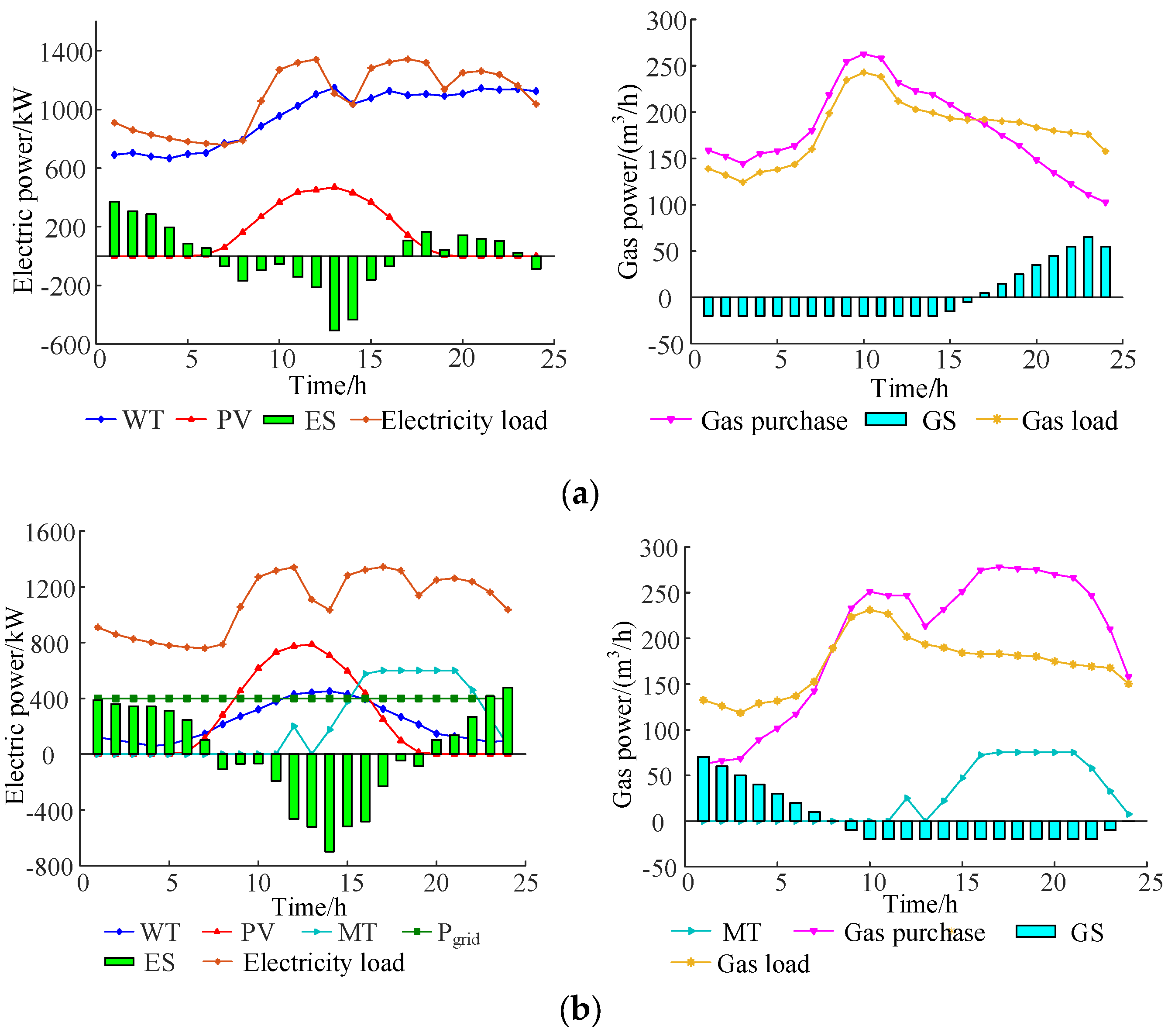
Let the renewable energy penetration rate requirement θ_ref = 50%, take the annual investment and operation cost f₁ and carbon emission f₂ of the IEGES as the optimization objectives to solve scheme 1, and obtain the Pareto sets as shown in Figure 5. From the figure, it can be seen that the IEGES cost f₁ and carbon emissions f₂ are obviously negatively correlated, and a decrease in cost f₁ will inevitably lead to an increase in carbon emissions f₂, and vice versa, and the simulation results are in line with reality. Among them, ε is obtained through the fixed-step method in Figure 5a and obtained by polynomial fitting in Figure 5b. Comparing the two, it can be concluded that the proposed method has a positive effect on improving the characteristics of the distribution of the Pareto front.

Taking ω^P = (0.5, 0.5) and the number of Pareto solutions m = 13, the fuzzy entropy weight method and fuzzy affiliation degree method are used to find the optimal solution among the obtained Pareto solutions. The optimization results of the four schemes are obtained as shown in

Table 2. Comparison of optimization results of different schemes.

Comparison	f1/×107 CNY	f2/×105 kg	θ	u
Scheme 1	2.2593	7	0.6496	0.8384
Scheme 2	2.5737	7	0.7105	0.5784
Scheme 3	2.6783	7	0.76	0.4603
Scheme 4	2.1947	7	0.7233	0.6472

, and the specific configuration results are shown in

Table 3. Optimal configuration results of different schemes.

Comparison	WT/kW	PV/kW	MT/kW	ES/kWh	GS/Nm3	P2G/kW	CC/kW
Scheme 1	1150	900	600	700	10	200	150
Scheme 2	3400	900	300	1200	30	480	/
Scheme 3	3480	1000	300	1300	0	/	/
Scheme 4	1780	950	500	850	15	250	60

. As can be seen from Table 2, the optimal results of f₂ in all schemes are the same, this is because the improved ε-constraint is adopted in this study to convert the proposed multi-objective model into a single-objective model (as shown in Section 3.2). For comparisons of different schemes, the same ε is selected for all schemes. Thus, the optimal results shown in Table 2 are reasonable. Specifically, scheme 1 has the smallest annual investment and operating cost, which is CNY 2.2593 × 10⁷. Although the renewable energy penetration (i.e., θ) of scheme 2 and scheme 3 is greater than that of scheme 1, the renewable energy utilization (i.e., u) is much lower than that of scheme 1, which is only 57.84% and 46.03% of the available amounts. This is because scheme 2 and scheme 3 are configured with a large number of WT and PV units to reduce the IEGES carbon emissions when the carbon emissions f₂ are given. According to Table 3, moreover, the renewable energy installation of scheme 2 and scheme 3 is 2.1 and 2.2 times larger than that of scheme 1, respectively, which leads to the case that a large amount of renewable energy is abandoned, whereas scheme 1 improves the utilization of renewable energy to a large extent by configuring 150 kW of CC and 200 kW of P2G. Moreover, it can be seen that although the annual cost of scheme 4 is lower than that of scheme 1, both the renewable energy penetration and the renewable energy utilization of scheme 4 are much worse. This is because in scheme 4, only the operational carbon emission is considered, the WT and PV units are regarded as zero-carbon resources; thus, more WT and PV units (i.e., 1.33 times greater than the renewable energy capacities of scheme 1 as shown in Table 3) are configured to reduce the IEGES carbon emissions, which directly deteriorated the renewable energy penetration index and the renewable energy utilization index of the IEGES system.

Based on the wind power, solar power, electric load and gas load data, the optimized power outputs of IEGES under different typical days are shown in Figure 6. Taking scenario 4 as an example, we can find that during the 00:00~15:00 time period, the WT and PV outputs are greater than the electric load, and the surplus power in this period is balanced by ES, P2G and CC. Specifically, P2G is put into operation to consume wind power in the time period 02:00~04:00 and the time period 11:00~15:00; correspondingly, P2G generates natural gas in these time periods, which facilitates the consumption of wind power. Similarly, CC is put into operation in the 11:00~15:00 time period, which improves the utilization of renewable energy. During the time period 19:00~24:00, there is no wind and no solar, the electricity load is balanced by ES and MT and power is purchased from the power grid. For the gas balance, although the gas demand increases at these time periods, the gas purchase does not increase, which is mainly due to the gas storage.

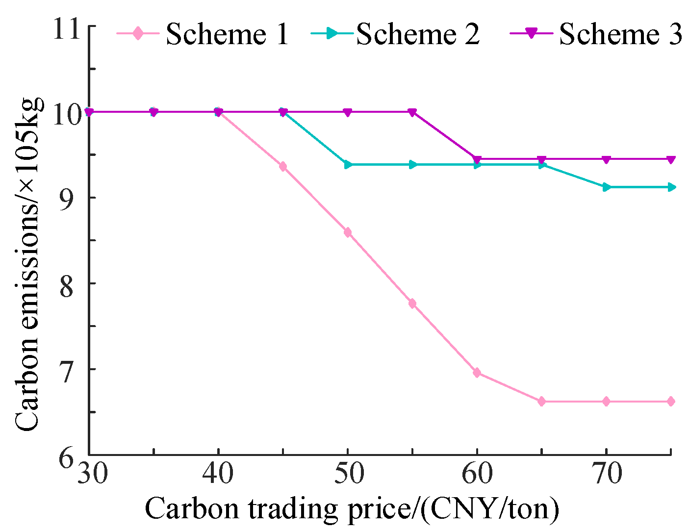
5.4. Analysis of the Impact of Carbon Trading Price on Optimization Results

In the simulation in this paper, it is assumed that the carbon trading price α_carb is fixed. In practice, the carbon trading price will fluctuate; thus, the trend of carbon emissions with carbon trading price under different schemes is presented in Figure 7. When the carbon trading price changes in the range of 30~40 CNY/t, the carbon emissions of the three schemes are at the upper limit due to the low penalty cost of carbon emissions. With the rise in carbon trading price, the penalty cost of carbon emissions increases accordingly, and the carbon emissions under scheme 1 are significantly reduced while the carbon emissions for scheme 2 and scheme 3 show a small decrease, which demonstrates that the proposed scheme can reduce carbon emissions effectively.

6. Conclusions

This paper focuses on the low-carbon planning problem of the IEGES. The life-cycle carbon emission models of each component in the IEGES are established, and a multi-objective optimal configuration model considering minimizing carbon emissions and minimizing the annual investment and operation costs is proposed. Through the numerical analysis, the following conclusions are obtained:

(1)

For the established multi-objective optimal configuration model, an optimal Pareto solution approach based on the fuzzy entropy weight method and the fuzzy affiliation degree is proposed. By comparing it with the existing fixed-step method, it is clear that the proposed method with polynomial fitting has a positive effect on improving the uniformity of the distribution of Pareto frontier solutions.

(2)

By comparing the three configuration schemes, it is obtained that the configuration of P2G and CC has a significant effect on the carbon emission reductions and renewable energy utilization of the IEGES. Moreover, the consideration of life-cycle carbon emissions makes the planning results more realistic compared with the scheme in which only the operational carbon emissions are considered.

(3)

In this study, the carbon trading price is critical to the planning results. By analyzing the effect of carbon trading price on the optimization results, it is obtained that the IEGES can reduce the carbon emission of the system remarkably through the introduction of the carbon trading mechanism.

Note that in this study, we assume that the carbon trading price is fixed, but in practice, the carbon trading price is affected by the carbon market scales, the carbon trading mechanism, new technology applications, etc. Moreover, for the modelling of life-cycle carbon emissions, the evolutionary patterns of the life-cycle carbon emissions are not included. In the context of the growing penetration of renewable energy and the decreasing carbon emissions in construction and recycling process, the evolutionary patterns of the life-cycle carbon emissions will bring significant impacts on the optimization results. Thus, future work will take carbon trading and the evolutionary patterns of the life-cycle carbon emissions and their impacts into consideration. Moreover, from the practical application perspective, the extended implementation of the proposed multi-objective optimal allocation method in specific scenarios (e.g., comprehensive buildings and microgrids) will be further investigated.

References

- Chan, C.C.; Zhou, G.Y.; Zhang, D. Intelligent energy ecosystem based on carbon neutrality. In Proceedings of the 2017 IEEE Conference on Energy Internet and Energy System Integration (EI2), Beijing, China, 26–28 November 2017; pp. 1–5. [Google Scholar]
- Zhong, Z.; Fang, J.; Hu, K.; Huang, D.; Ai, X.; Yang, X.; Wen, J.; Pan, Y.; Cheng, S. Power-to-Hydrogen by Electrolysis in Carbon Neutrality: Technology Overview and Future Development. CSEE J. Power Energy Syst. 2023, 9, 1266–1283. [Google Scholar] [CrossRef]
- Jelinek, T.; Bhave, A.; Buchoud, N.; Bühler, M.M.; Glauner, P.; Inderwildi, O.; Kraft, M.; Mok, C.; Nübel, K.; Voss, A. International Collaboration: Mainstreaming Artificial Intelligence and Cyberphysical Systems for Carbon Neutrality. IEEE Trans. Ind. Cyber-Phys. Syst. 2024, 2, 26–34. [Google Scholar] [CrossRef]
- Liu, J. Development path of power intelligence supporting the construction of new power system. Energy Sci. Technol. 2022, 20, 3–7. [Google Scholar]
- Lin, S.; Liu, C.; Shen, Y.; Li, F.; Li, D.; Fu, Y. Stochastic Planning of Integrated Energy System via Frank-Copula Function and Scenario Reduction. IEEE Trans. Smart Grid 2022, 13, 202–212. [Google Scholar] [CrossRef]
- Peng, K.; Zhang, C.; Xu, B.; Chen, Y.; Zhao, X. Status and prospect of pilot projects of integrated energy system with multi-energy collaboration. Electr. Power Autom. Equip. 2017, 37, 3–10. [Google Scholar]
- Saif, A.; Khadem, S.K.; Conlon, M.F.; Norton, B. Impact of Distributed Energy Resources in Smart Homes and Community-Based Electricity Market. IEEE Trans. Ind. Appl. 2023, 59, 59–69. [Google Scholar] [CrossRef]
- Riaz, S.; Mancarella, P. Modelling and Characterisation of Flexibility From Distributed Energy Resources. IEEE Trans. Power Syst. 2022, 37, 38–50. [Google Scholar] [CrossRef]
- Qiu, Y.; Li, Q.; Ai, Y.; Chen, W.; Benbouzid, M.; Liu, S.; Gao, F. Two-stage distributionally robust optimization-based coordinated scheduling of integrated energy system with electricity-hydrogen hybrid energy storage. Prot. Control Mod. Power Syst. 2023, 8, 33. [Google Scholar] [CrossRef]
- Qin, M.; Yang, Y.; Zhao, X.; Xu, Q.; Yuan, L. Low-carbon economic multi-objective dispatch of integrated energy system considering the price fluctuation of natural gas and carbon emission accounting. Prot. Control Mod. Power Syst. 2023, 8, 61. [Google Scholar] [CrossRef]
- Zhang, Y.; Han, Y.; Liu, D.; Dong, X. Low-Carbon Economic Dispatch of Electricity-Heat-Gas Integrated Energy Systems Based on Deep Reinforcement Learning. J. Mod. Power Syst. Clean Energy 2023, 11, 1827–1841. [Google Scholar] [CrossRef]
- Wang, S.; Ding, Y.; Ye, C.; Wan, C.; Mo, Y. Reliability evaluation of integrated electricity–gas system utilizing network equivalent and integrated optimal power flow techniques. J. Mod. Power Syst. Clean Energy 2019, 7, 1523–1535. [Google Scholar] [CrossRef]
- Li, Q.; Mao, Y.; Liu, Y.; Zhang, A.; Yang, W. Modeling of Integrated Energy System of Offshore Oil and Gas Platforms Considering Couplings Between Energy Supply System and Oil and Gas Production System. IEEE Access 2020, 8, 157974–157982. [Google Scholar] [CrossRef]
- Yan, C.; Bie, Z.; Liu, S.; Urgun, D.; Singh, C.; Xie, L. A Reliability Model for Integrated Energy System Considering Multi-energy Correlation. J. Mod. Power Syst. Clean Energy 2021, 9, 811–825. [Google Scholar] [CrossRef]
- Zhao, Y.; Wang, C.; Zhang, Z.; Lv, H. Flexibility Evaluation Method of Power System Considering the Impact of Multi-Energy Coupling. IEEE Trans. Ind. Appl. 2021, 57, 5687–5697. [Google Scholar] [CrossRef]
- Dong, W.; Lu, Z.; He, L.; Zhang, J.; Ma, T.; Cao, X. Optimal Expansion Planning Model for Integrated Energy System Considering Integrated Demand Response and Bidirectional Energy Exchange. CSEE J. Power Energy Syst. 2023, 9, 1449–1459. [Google Scholar] [CrossRef]
- Dou, X.; Wang, J.; Zhang, Z.; Gao, M. Optimal configuration of multitype energy storage for integrated energy system considering the system reserve value. CSEE J. Power Energy Syst. 2022. [Google Scholar] [CrossRef]
- Li, Z.; Wang, C.; Li, B.; Wang, J.; Zhao, P.; Zhu, W.; Yang, M.; Ding, Y. Probability-Interval-Based Optimal Planning of Integrated Energy System With Uncertain Wind Power. IEEE Trans. Ind. Appl. 2020, 56, 4–13. [Google Scholar] [CrossRef]
- Xuan, A.; Shen, X.; Guo, Q.; Sun, H. Two-Stage Planning for Electricity-Gas Coupled Integrated Energy System With Carbon Capture, Utilization, and Storage Considering Carbon Tax and Price Uncertainties. IEEE Trans. Power Syst. 2023, 38, 2553–2565. [Google Scholar] [CrossRef]
- Zhang, D.; Zhu, H.; Zhang, H.; Goh, H.H.; Liu, H.; Wu, T. Multi-Objective Optimization for Smart Integrated Energy System Considering Demand Responses and Dynamic Prices. IEEE Trans. Smart Grid 2022, 13, 1100–1112. [Google Scholar] [CrossRef]
- Yang, Y.; Luo, Z.; Yuan, X.; Lv, X.; Liu, H.; Zhen, Y.; Yang, J.; Wang, J. Bi-Level Multi-Objective Optimal Design of Integrated Energy System Under Low-Carbon Background. IEEE Access 2021, 9, 53401–53407. [Google Scholar] [CrossRef]
- Wang, Y.; Wang, Y.; Huang, Y.; Yu, H.; Du, R.; Zhang, F.; Zhang, F.; Zhu, J. Optimal Scheduling of the Regional Integrated Energy System Considering Economy and Environment. IEEE Trans. Sustain. Energy 2019, 10, 1939–1949. [Google Scholar] [CrossRef]
- Ding, X.; Zhang, X.; Wang, S.; Wang, C.; Xiong, H.; Guo, C. Low-carbon planning of regional integrated energy system considering optimal construction timing under dual carbon goals. High Volt. Eng. 2022, 48, 2584–2596. [Google Scholar]
- Zhang, X.; Liu, X.; Zhong, J. Integrated energy system planning considering a reward and punishment ladder-type carbon trading and electric-thermal transfer load uncertainty. Proc. CSEE 2020, 40, 6132–6141. [Google Scholar]
- Wen, M.; Hu, Z.; Long, Y.; Li, Y.; Jiang, T.; Wang, Y. Optimal planning of integrated energy system considering carbon emission penalty factor. J. Electr. Power Sci. Technol. 2021, 36, 11–18. [Google Scholar]
- Wang, Z.; Teng, Y.; Yan, J.; Jin, H.; Chen, Z. A new rural energy system planning method with consideration of energy resource cost and carbon emission trading benefit synergies. Proc. CSEE 2022, 42, 7074–7087. [Google Scholar]
- Yang, J.; Zhang, N.; Wang, Y.; Kang, C. Multi-energy system towards renewable energy accommodation: Review and prospect. Autom. Electr. Power Syst. 2018, 42, 11–24. [Google Scholar]
- Luo, J.; Lu, C.; Meng, F. Generation expansion planning and its benefit evaluation considering carbon emission and coal supply constraints. Autom. Electr. Power Syst. 2016, 40, 47–52. [Google Scholar]
Figure 1.
Schematic diagram of IEGES.
Figure 2.
The annual wind speed and solar intensity data: (a) annual wind speed data; (b) annual solar intensity data.
Figure 3.
Electricity load and gas load in a typical day.
Figure 4.
Typical scenario clustering results of electric load.
Figure 5.
Results of Pareto sets in scheme 1: (a) calculating ε with fixed-step method, (b) calculating ε with fitting-based method.
Figure 6.
The power outputs of IEGES in different scenarios: (a) Scenario 1, (b) Scenario 2, (c) Scenario 3, (d) Scenario 4.
Figure 7.
The trend of carbon emissions changing with carbon trading price.