Numerical Simulation of the Mixing and Salt Washing Effects of a Static Mixer in an Electric Desalination Process

Abstract

Electric desalination units in the crude oil refining process are becoming increasingly important with the growing trend towards heavy and poor crude oils. The oil–water mixing effect of the static mixer plays a crucial role in the electric desalination process. The present study investigated the effect of various variables, such as mixer type, number of mixing elements, washing water consumption, and oil viscosity and density on the oil–water mixing efficiency of a static mixer. In addition, this study also analyzed the effect of these variables on the salt washing process that occurs during mixing using a kinetic equation for the dissolution of inorganic salts. The results showed that the number of mixing elements was the most significant variable, followed by the amount of washing water injected. The density of the crude oil had a negligible effect. Based on these results, the use of four mixing elements in the SMX static mixer was recommended. The injection of washing water should be controlled at about 8%, while ensuring that the interfacial tension between oil and water remains below 0.01 N/m. Under these conditions, the salt washing efficiency reached 46.3%. This study provides a theoretical basis for designing static mixers and optimizing their operation in electric desalination processes.

1. Introduction

Worldwide, major oil fields are generally in the middle and late stages of production, which means that the quality of crude oil tends to be heavier and poorer [1]. The salt and water content of crude oil has also increased due to the implementation of various measures to increase production [2,3,4]. A gradual increase in the salt content of crude oil can lead to numerous hazards during the subsequent processes. For example, it can cause scaling on the heat exchanger tube wall, which can clog the tubes and reduce heat transfer efficiency. It can poison and deactivate the catalysts, resulting in lower product conversion rates and inferior products [5]. It can also cause significant corrosion of equipment [6]. At the same time, crude oil with a higher water content not only increases energy consumption during the refining process but also causes excessive vapor phase loading in the distillation tower due to the instantaneous evaporation of a large amount of water, leading to tower flushing accidents. Therefore, the requirements for desalination and dehydration of crude oil in the refining process are increasing [7,8].

The oil industry currently uses electric desalination units for crude oil pre-treatment in oil fields and refineries [9]. The electric desalination process uses a static mixer to thoroughly mix crude oil and washing water, dissolve the salt in the crude oil, and then separate the oil and water in the electric desalination tank through the combined action of the electric field and the gravity field to remove salt and water [10]. To save energy and water and reduce the load on the electric desalination process, the amount of washing water injected is generally 3–12%. The performance of the static mixer is crucial in the electric desalination process [11,12].

Most of the studies on static mixers have been carried out using Computational Fluid Dynamics (CFD), except for Hammoudi’s work, which is experimental (

Table 1. Summary of research on the process analysis of the static mixer.

Researchers	Factor	Conclusion
Hammoudi et al. [13]	SMX static mixer, Reynolds number	The mixing performance is good at Reynolds numbers greater than 4500.
Nasser A. A et al. [14]	The installation method for the static mixer in the electric desalination process	A total saving of more than 8.5 million gallons of wash water was achieved during the nine months of the field trial.
Wang et al. [15]	Aspect ratio, the central center position of elements	When the central position of the elements is changed, the blending effect will improve.
Jiang et al. [16]	Thickness of mixing element	The thickness of the mixing elements significantly affects the flow field.
Lowry et al. [17]	Roughness of mixing element	With the static mixer, roughness had up to a 60% contribution to the overall pressure loss.
Chakleh et al. [18]	Types of static mixers	The performance of SMV static mixers is superior to that of SK static mixers and other recently developed static mixers.
Moghaddam [19]	Types of static mixers	The SMX static mixer is superior to both the INLINER SERIES 45 static mixer and the KOMAX static mixer.
Liu et al. [20]	The number of mixing elements	To balance pressure loss and mixing uniformity, it is recommended to use four mixing units.
Zalc, J. M. et al. [21]	Feeding methods, feeding positions, the number of mixing elements	When the level of mixing reaches a certain point, adding more mixing elements does not significantly improve the mixing effect.
Valdes et al. [22]	Oil–water interfacial tension	The mixing effect of liquid–liquid two-phase flow through the static mixer is affected by the amount of surfactant used.
Jegatheeswaran et al. [23]	Viscosity of the liquid	When mixing liquids of varying viscosities, the energy required to achieve the desired mixing state increases with the viscosity of the liquids.

) [13,14]. However, these studies mainly focus on the influence of static mixers (such as the shape and thickness of the mixing elements [15,16] and the type [17,18,19]) and the properties of the mixed liquid [20,21,22,23] on the oil–water mixing effect, and they only discuss the transmission process without delving into the mass transfer process of salt washing efficiency in the electric desalination process.

The basic purpose of using static mixers in the electrical desalination process is to wash out the salt particles suspended in the crude oil. The oil and water are made sufficiently turbulent by the static mixer to ensure that the wash water comes into contact with the salt particles suspended in the crude oil, thereby dissolving the salt in the water and achieving the desired result of salt washing.

The static mixers currently used in the electrical desalination process include the SMX, SMV, and SSK types. The efficiency of oil–water mixing can be improved by increasing the number of mixing elements.

In our case, the research should not only focus on the mixing process but also on the mass transfer of salt from oil to water. As such, we introduce the salt dissolution kinetics using a User-Defined Function (UDF) and analyze the mixing process and mass transfer process simultaneously to provide data guidance for the selection of the static mixer in the electric desalination process.

As such, we will investigate the effect of static mixer morphology, crude oil properties, and washing water properties on the characteristics of the oil–water two-phase flow characteristics and salt mass transfer performance. This will provide a theoretical basis for the design and optimization of static mixers and their operation.

2. Materials and Methods

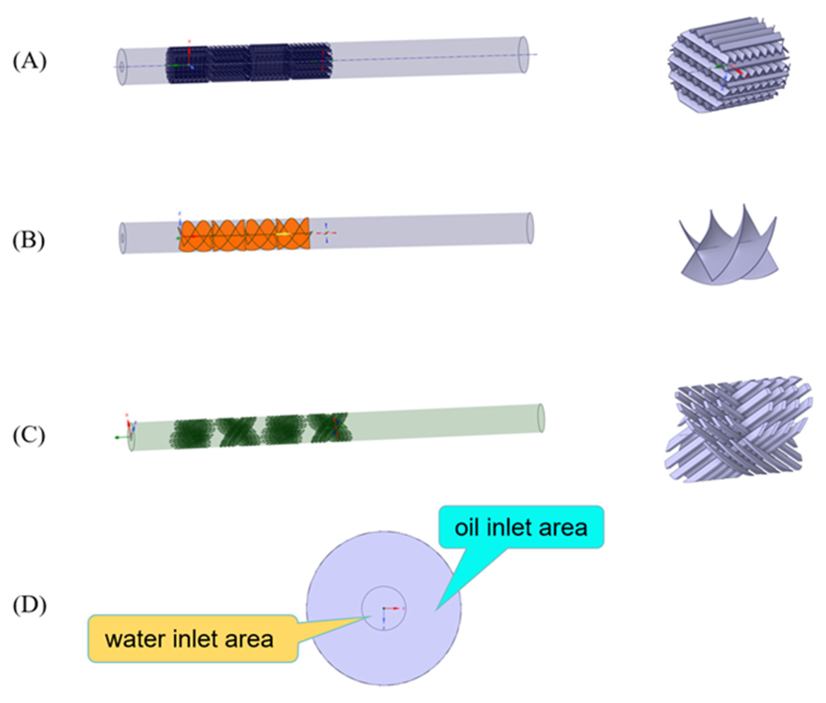
2.1. Physical Model and Boundary Conditions

This study simulated three types of static mixers, namely SMX, SMV, and SSK, each with the same blade thickness composition and a total pipe diameter of 550 mm. The stabilization zone is set before and after the mixing of the internal components, resulting in a total pipe length of 9000 mm for each model. The front stabilization zone has a length of 1000 mm, and each mixing element has a radial length of 950 mm. The geometric meshes of the three models are shown in Figure 1.

Table 2. Properties of crude oils used in the simulation.

Property	Value
Density (393.15 K)	880 kg/m3
Viscosity (393.15 K)	0.002 kg/(m·s)
Specific heat capacity	1845 J/(kg·K)
Oil–water interfacial tension	0.01 N/m

lists the crude oil properties. For the washing water properties, water–liquid is selected from the Fluent database, and for the salt properties, NaCl is selected from the Fluent database. The oil component consists of crude oil and salt, while the water component consists of water and salt. The pipeline has a small circular water inlet with a diameter of 150 mm, and the rest of the area is the oil inlet area, as shown in Figure 1D. The oil inlet area is 12.44 times larger than the water inlet area. Both inlets are set up as velocity inlets, with the inlet velocity of the oil component set at 2 m/s and the inlet velocity of the water component set at 2.5 m/s. The water–oil ratio is 10.04%. The pressure outlet is configured for natural outflow.

2.2. Computational Method and Assumptions

The flow field is calculated using the Fluent 14.5 software. The Eulerian multiphase flow and turbulence models are selected from the Realizable k-epsilon model, while the wall function is selected from the Standard Wall Function (SWF) [24]. The pressure-based SIMPLE algorithm is used to calculate the flow field iteratively, and the pressure, momentum, and energy equations are solved using the second-order windward algorithm. The mixing element and the wall surface are chosen as the static and fixed wall surfaces, respectively. For the computational method, the turbulence equations of the numerical simulation are based on the Realizable k-epsilon model. This model is better equipped to handle fast strain flow and provides a more accurate prediction of the flow distribution for flat plates and cylindrical jets. It also performs well for rotating flow, boundary-layer flow with a strong back pressure gradient, flow separation, and secondary flow.

The continuity and momentum equations [25] are as follows:

$$\nabla ·{(\mathsf{\alpha }}_{\mathrm{q}}{\mathsf{\rho }}_{\mathrm{q}}{u}_q)=0$$

(1)

$$\nabla ·{(\mathsf{\alpha }}_{\mathrm{q}}{\mathsf{\rho }}_{\mathrm{q}}{u}_q{u}_q)={\mathsf{\alpha }}_{\mathrm{q}}{\mathsf{\rho }}_{\mathrm{q}}\mathrm{g}-{\mathsf{\alpha }}_{\mathrm{q}}\nabla \mathrm{p}+\nabla ·{(\mathsf{\alpha }}_{\mathrm{q}}{\mathsf{\mu }}_{eff,q}\left(\nabla u_q+{\left(\nabla u_q\right)}^T\right)+F_q$$

(2)

$$\sum {\mathsf{\alpha }}_{\mathrm{q}}=1$$

(3)

where ${\mathsf{\alpha }}_{\mathrm{q}}$ is the qth-phase volume fraction, ${\mathsf{\rho }}_{\mathrm{q}}$ is the qth-phase density, $u_q$ is the velocity vector during the qth phase, g is the gravitational acceleration vector, F is the sum of the forces of all phases acting on the qth phase, P is the pressure, and ${\mathsf{\mu }}_{eff,q}$ is the effective viscosity. And, the effective viscosity is the sum of the continuous-phase molecular viscosity, ${\mathsf{\mu }}_q$, and the turbulent viscosity, ${\mathsf{\mu }}_t$.

$${\mathsf{\mu }}_{eff,c}={\mathsf{\mu }}_q+{\mathsf{\mu }}_t$$

(4)

The turbulence kinetic energy equation is as follows [25]:

$$\nabla ·({\mathsf{\alpha }}_{\mathrm{q}}{\mathsf{\rho }}_{\mathrm{q}}{k_{q}u}_q)=\nabla [({\mathsf{\mu }}_q+\frac{{\mathsf{\mu }}_t}{{\mathsf{\sigma }}_{k,q}})\nabla k_q]+{\mathrm{G}}_{\mathrm{k}}+{\mathrm{G}}_{\mathrm{b}}-\mathsf{\rho }\mathsf{\epsilon }-{\mathrm{Y}}_{\mathrm{M}}$$

(5)

$$\nabla ·({\mathsf{\alpha }}_{\mathrm{q}}{\mathsf{\rho }}_{\mathrm{q}}{k_{q}u}_q)=\nabla [(\mu +\frac{{\mu }_t}{{\sigma }_{\epsilon }})\nabla \mathsf{\epsilon }]+\rho C_{1\epsilon }S\epsilon -{\rho c}_2\frac{{\epsilon }^2}{k+\sqrt{v\epsilon }}+C_{1\epsilon }\frac{\epsilon }{k}{C}_{3\epsilon }{G}_b$$

(6)

where x is the turbulent kinetic energy; ${\mathrm{Y}}_{\mathrm{M}}$ is the radial pulsation expansion in turbulence; ${\mathrm{G}}_{\mathrm{k}}$ is the turbulent kinetic energy production term due to the mean velocity gradient; ${\mathrm{G}}_{\mathrm{b}}$ is the turbulent kinetic energy production term due to buoyancy; $\mathsf{\epsilon }$ is the turbulent dissipation rate; ${\mathsf{\sigma }}_{\mathrm{k}}$ and ${\mathsf{\sigma }}_{\mathsf{\epsilon }}$ represent the Planck numbers for the turbulent kinetic energy k and the dissipation rate $\mathsf{\epsilon }$, respectively; and ${\mathrm{C}}_{1\mathsf{\epsilon }}$, ${\mathrm{C}}_{2\mathsf{\epsilon }}$, and ${\mathrm{C}}_{3\mathsf{\epsilon }}$ are empirical constants.

The salt dissolution rate equation is as follows [26]:

$${\mathrm{W}}_{\mathrm{c}}=\mathrm{K}({\mathrm{C}}_{\mathrm{b}}-\mathrm{C})/\left(3600\mathsf{\rho }\right)$$

(7)

where ${\mathrm{W}}_{\mathrm{c}}$ is the salt dissolution rate in contact with water (m/s); K is the salt dissolution coefficient (m/h), chosen as 0.0785; ${\mathrm{C}}_{\mathrm{b}}$ is the standard saturated brine concentration, chosen as 315 kg/m³; C is the salt concentration in the wash water (kg/m³); and $\mathsf{\rho }$ is the current density of the wash water (kg/m³).

This study is based on the following main assumptions:

(1)

The acceleration due to gravity is $9.81 \mathrm{m}/{\mathrm{s}}^2$ downwards along the z-axis.

(2)

In Newtonian fluid dynamics, each fluid in a multiphase flow has a constant physical property. This implies that both are incompressible fluids. The slip velocity at the interphase is set by default to the no-slip condition [27,28].

(3)

The surface tensions of the oil and water are set to a fixed value of $0.01 \mathrm{N}/\mathrm{m}$.

(4)

All surfaces in each static mixer are smooth and frictionless. Only their turbulence-inducing effects on the cutting and guiding of fluid flow are considered [29,30].

(5)

The effect of the radiative heat transfer is neglected.

(6)

The oil is in a mixed state and acts as a continuous phase. The formation of oil-in-water emulsions is unexpected in this process.

(7)

It is assumed that the temperature remained constant during the oil–water mixing process.

(8)

According to the model scale, the effect of salt component transport on the heat change is negligible.

(9)

The effect of salt transport on the volume change of the two fluids is negligible.

2.3. Grid Irrelevance Test and Model Feasibility Analysis

The analysis of the CFD simulation focused on the fluid domain. The fluid domain model developed using geometric drafting software was imported into the mesh generation software for meshing. The mesh was then imported into the Fluent software for simulation.

A limited number of meshes can lead to distortion of the simulation results. However, as the number of meshes increases, the accuracy of the calculations improves, although this may increase the cost of the calculations. A mesh irrelevance test is required to select an appropriate number of meshes. As the mesh size decreases, the number of meshes to be divided simultaneously increases. For the mesh sizes, 15 mm, 12 mm, 10 mm, and 5 mm are selected in turn. The oil–water mixing in the static mixer simulation is then carried out, and the pressure drop at both ends of the static mixer is used as a criterion. If the pressure difference between the two ends of the static mixer is close in two calculations, it is assumed that the mesh size has no effect on the calculation’s accuracy.

Different meshing criteria are used to ensure the mesh independence of the SMX static mixer and to reduce the computational errors due to meshing. The CFD simulation results of the models with different grid sizes are compared by analyzing the inlet and outlet pressure drops.

Table 3. The differential pressure at both ends of a static mixer with various grid sizes.

Grid Size/mm	15	12	10	5
Number of meshes	838,452	1,386,572	2,158,364	7,254,231
Pressure drop/kPa	114.7	118.2	117.6	117.8

shows that the variation of the static mixer differential pressure is 0.2% in the 10 mm grid size model compared to the 5 mm grid size model. This indicates that the mesh irrelevance requirement has been met for the 10 mm grid size.

In an actual production situation, the differential pressure at both ends of the static mixer is within the range of 118 to 120 kPa. The pressure drop in the static mixer during crude oil salt washing under operating conditions is simulated to be 117–118 kPa, which is close to the actual production situation. This means that the selected model and boundary conditions are reliable for the numerical simulation of the static mixer calculation.

2.4. Characterization Methods

In this study, the performance of a static mixer is evaluated in three main ways. Firstly, the mixing effect of the static mixer is evaluated to determine its suitability for oil–water mixing. Secondly, an evaluation of the differential pressure at both ends of the static mixer is critical in determining the energy consumption of the static mixer. This will determine the cost of using the static mixer. Finally, an evaluation of the salt washing efficiency is carried out, which is a critical factor in determining whether the static mixer will meet the requirements of the electrical desalination process.

2.4.1. Mixing Effect

Firstly, the evaluation of the performance of the static mixer is primarily based on the mixing effect. Mixing uniformity is one of the most important parameters to characterize the mixing performance. The most common measure used to describe mix homogeneity is the coefficient of variation (CoV), which shows the deviation from the average mix composition. The CoV can be determined based on statistical analysis using the following equation [31]:

$$\mathrm{C}\mathrm{o}\mathrm{V}=\frac{\mathsf{\sigma }}{\overline{\mathrm{x}}}\times 100\%$$

$$\mathsf{\sigma }=\sqrt{\frac{\sum _{\mathrm{n}=1}^{\mathrm{N}}{({\mathrm{x}}_{\mathrm{i}}-\overline{\mathrm{x}})}^2}{\mathrm{N}-1}}$$

(8)

In this paper, N, the number of sampling points at the outlet, is set to 2000. ${\mathrm{x}}_{\mathrm{i}}$ is the volume fraction of the crude oil components at the sampling point, and $\overline{\mathrm{x}}$ is the average volume fraction of the crude oil at the outlet. The smaller the CoV value, the better the mixing effect.

2.4.2. Salt Washing Effect

The efficiency of the salt washing process is assessed according to the value of salt washing efficiency (SWE). A higher SWE value indicates a more effective desalting process for the oil.

$$\mathrm{S}\mathrm{W}\mathrm{E}=1-\frac{\int {\mathsf{\alpha }}_{\mathrm{o}\mathrm{i}\mathrm{l}\mathrm{c}}{\mathrm{m}}_{\mathrm{o}\mathrm{i}\mathrm{l}\mathrm{c}}\mathrm{d}\mathrm{s}}{\int {\mathsf{\alpha }}_{\mathrm{o}\mathrm{i}\mathrm{l}1}{\mathrm{m}}_{\mathrm{o}\mathrm{i}\mathrm{l}1}\mathrm{d}\mathrm{s}}$$

(9)

where ${\mathsf{\alpha }}_{\mathrm{o}\mathrm{i}\mathrm{l}\mathrm{c}}$ is the salt mass fraction in the oil phase at the outlet cross-section grid, ${\mathrm{m}}_{\mathrm{o}\mathrm{i}\mathrm{l}\mathrm{c}}$ is the input oil mass per unit time at the outlet cross-section grid, ${\mathsf{\alpha }}_{\mathrm{o}\mathrm{i}\mathrm{l}1}$ is the salt mass fraction in the oil phase at the inlet cross-section grid, and ${\mathrm{m}}_{\mathrm{o}\mathrm{i}\mathrm{l}1}$ is the input oil mass per unit time at the inlet cross-section grid.

2.4.3. Differential Pressure

When the fluid flows through a static mixer, its design characteristics create significant frictional resistance, resulting in a significant pressure difference between the ends and energy loss. Therefore, the magnitude of the differential pressure of a static mixer is an important evaluation criterion. If the mixing requirements are met, the smaller the differential pressure between the two ends of the static mixer, the better its performance.

3. Results and Discussion

3.1. Effect of the Static Mixer

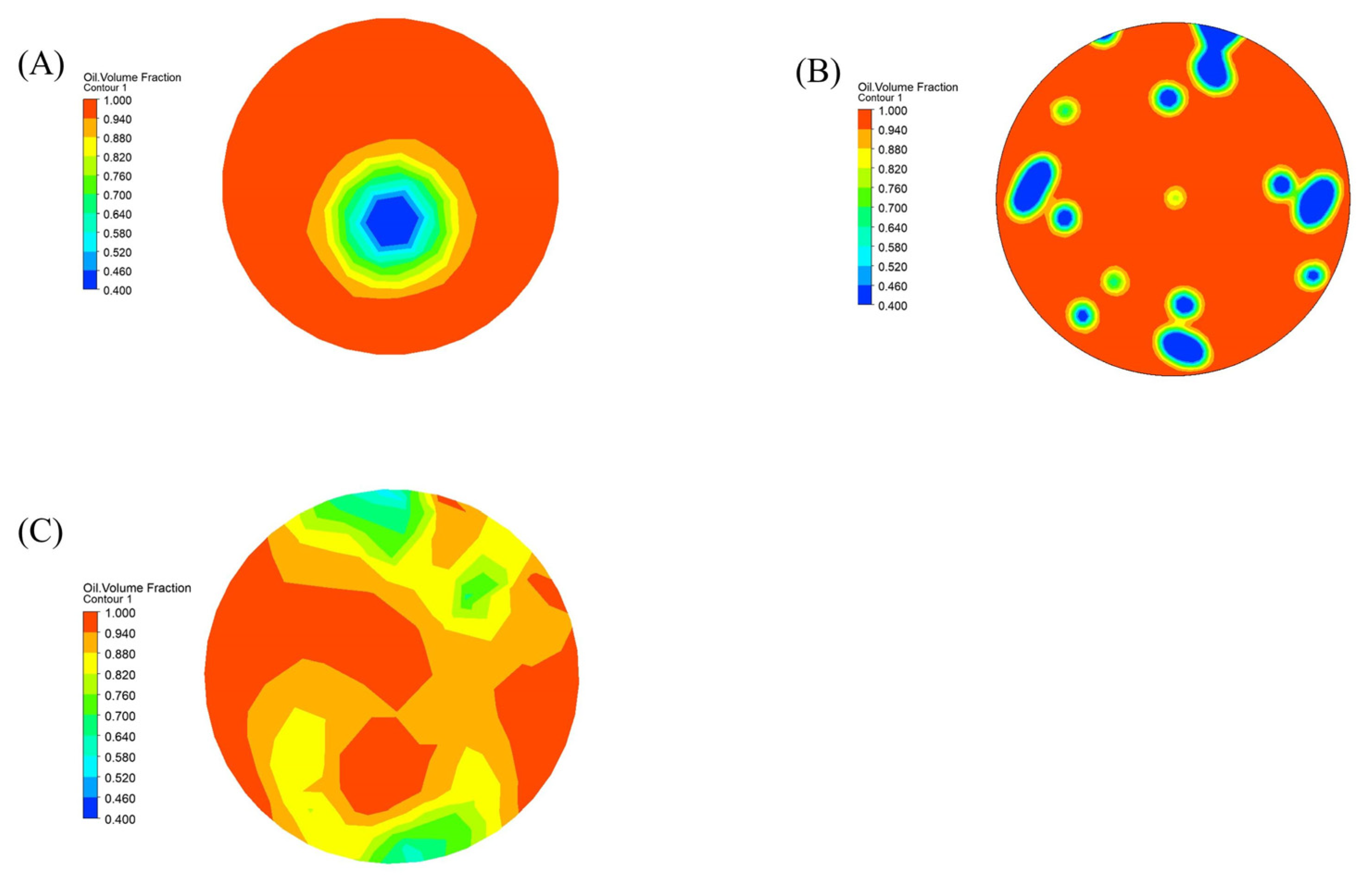
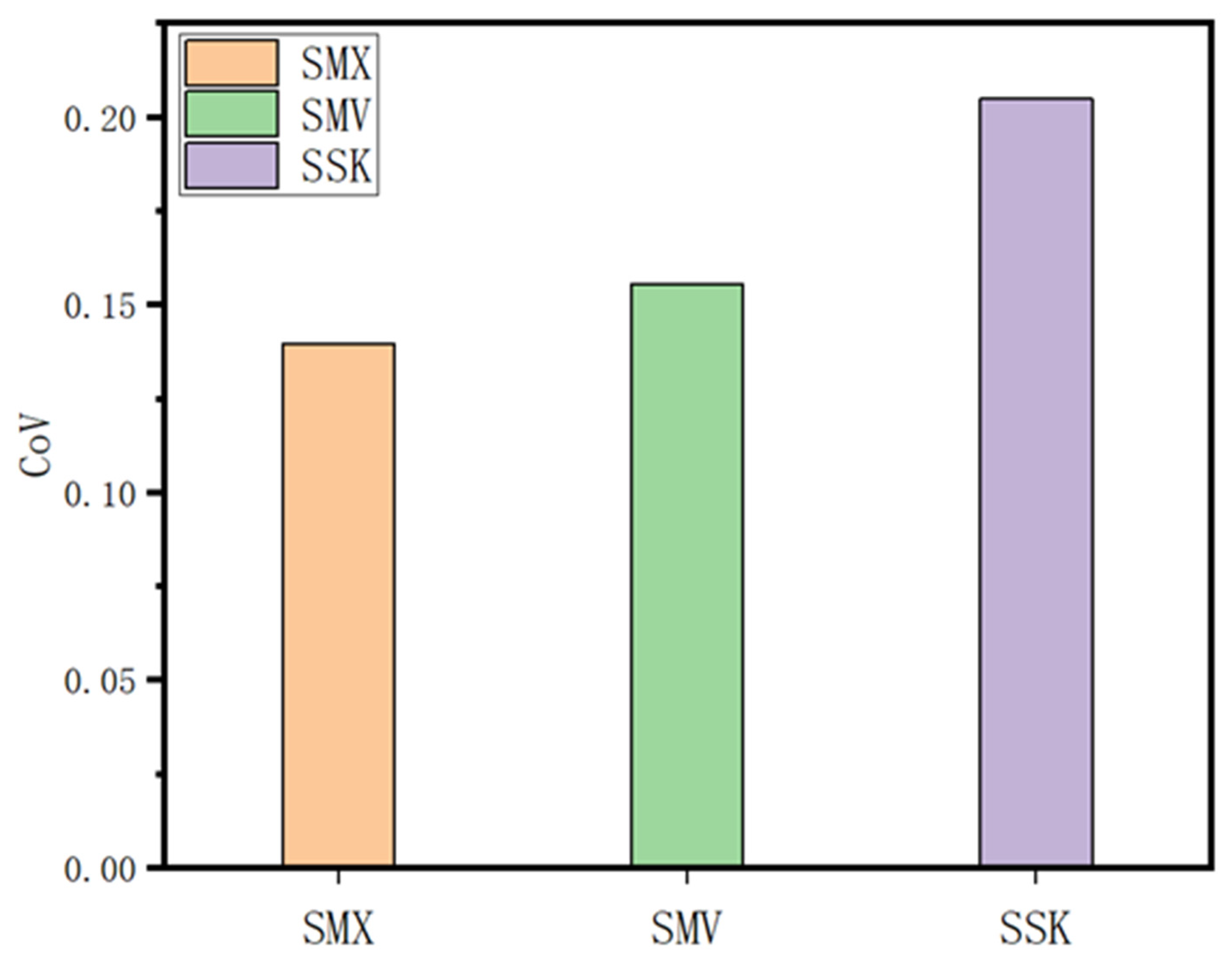
3.1.1. Type of Mixer

The mixing effect of an oil–water mixture with a water content of 10.04% after passing through the SMV, SMX, and SSK static mixers with four groups of mixing elements was investigated through CFD. Figure 2 shows the oil and water distribution at the outlet. It can be seen that the SMX and SMV static mixers had a better mixing effect than the SSK static mixer, as indicated by their lower CoV values (Figure 3). Figure 4 shows the radial pressure drop diagrams for the three types of static mixers; the SMV has a pressure drop of 2272.25 kPa, the SSK has a pressure drop of 29.19 kPa, and the SMX has a pressure drop of 118.36 kPa. The SMX static mixer has excellent mixing not only due to the effect of the morphology of its mixing elements but also because the pressure drop of this type of mixer is only 118.36 kPa, which is acceptable in industrial situations. The SMV static mixer provides effective mixing, but the pressure drop is too high, resulting in a significant increase in energy consumption. The SSK static mixer creates intense turbulence only at the interface of the two mixing elements, which promotes mixing of the oil and water. However, due to the lack of high-intensity turbulence and a more uniform flow field around the spiral blade, the SSK static mixer has the worst mixing effect despite having a minimum pressure drop at both ends. In summary, the SMX static mixer is considered the most suitable for the electric desalination process because of its excellent performance in the crude oil–water mixing process and because it meets the industrial requirements for differential pressure at both ends. In this study, the SMX static mixer is selected as the oil–water mixing device for the electric desalination process.

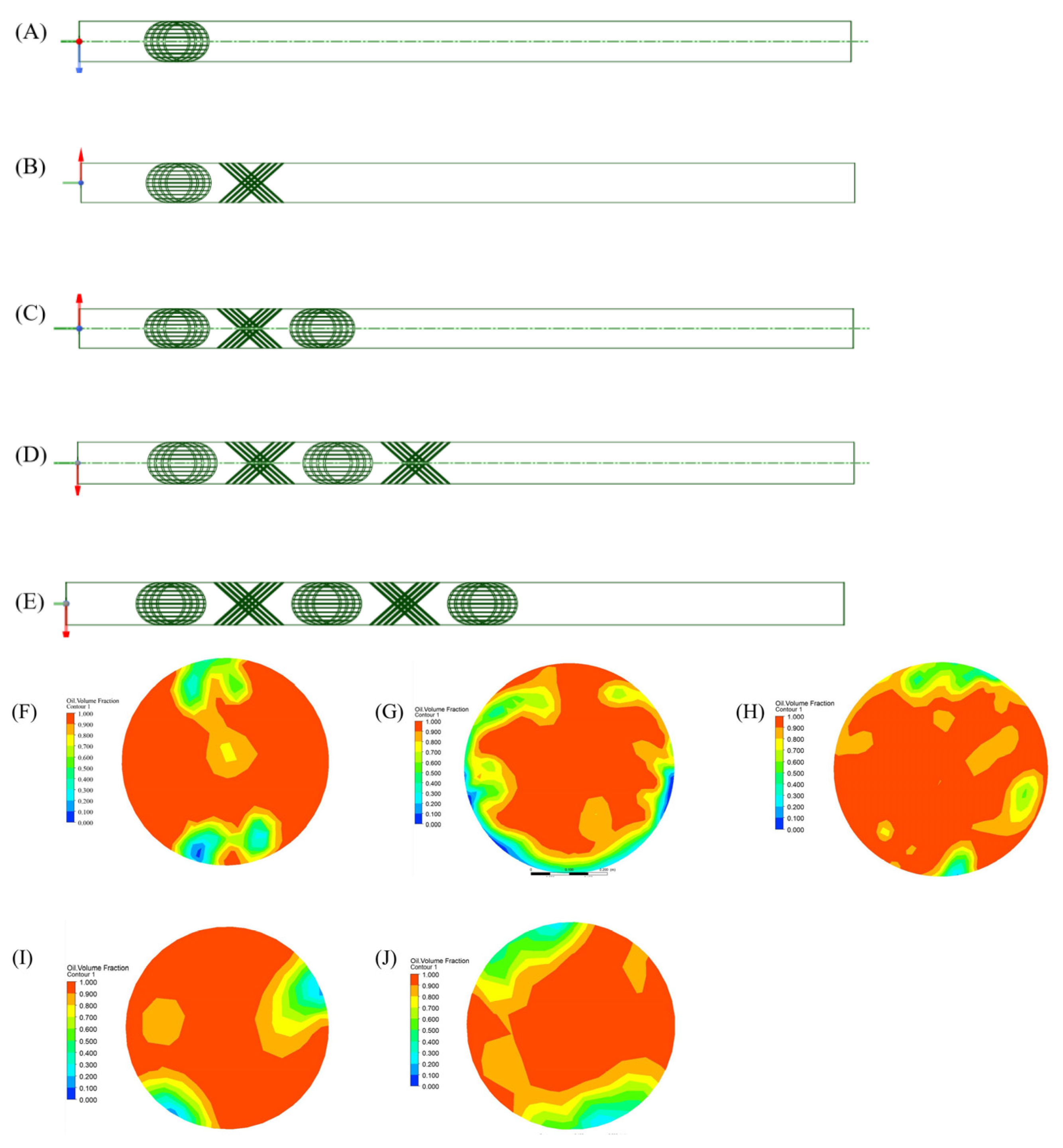
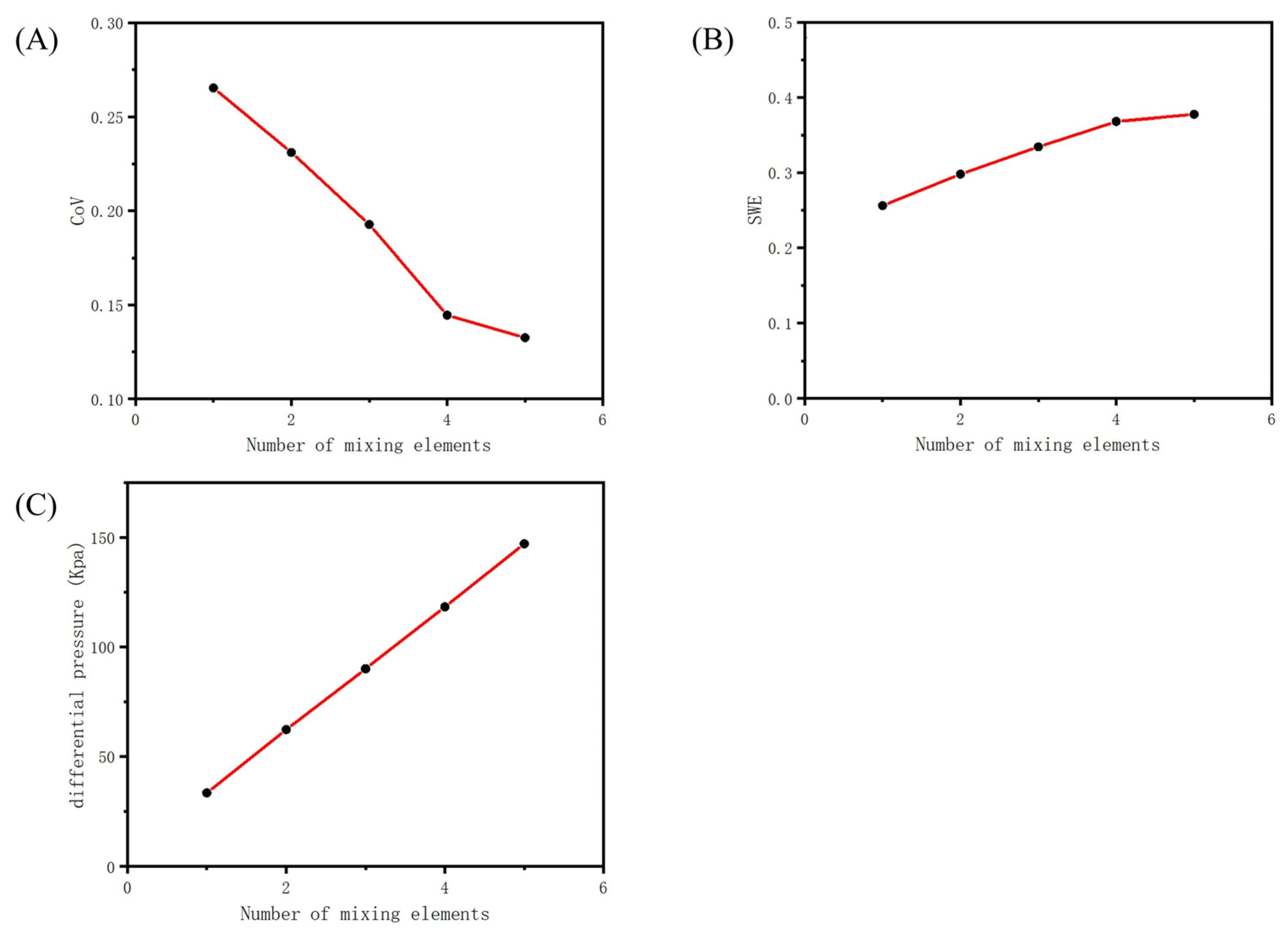
3.1.2. Number of Mixing Elements in the Mixer

Figure 5 shows five pipelines with different numbers of static mixer mixing elements used in the simulation experiment. The number of mixing elements ranged from one to five, with each element connected in a 90° rotated state. Oil is introduced at a velocity of 2 m/s with the same oil–water ratio as in the previous section. Simulations are carried out using static mixers with different numbers of mixing elements. The cloud diagram of the outlet region in Figure 5 clearly shows the changes in the oil–water mixing situation. It can be seen that the number of mixing elements has a direct effect on the oil–water mixing effect.

Figure 6A shows the effect of the number of mixing elements on the mixing effect. The CoV value decreased rapidly from one mixing element to two mixing elements and then changed more slowly between the four and five mixing elements. When the number of mixing elements reached four or more, increasing the number of mixing elements in the static mixer did not significantly improve the mixing effect of the system.

The effect of the number of mixing elements on salt washing was investigated by analyzing the SWE values. The results showed that increasing the number of mixing elements gradually improved the salt washing effect (Figure 6B). When the number of mixing elements is two, three, and four, the growth rates are 14.05%, 10.85%, and 9.13%, respectively. However, the growth rate decreases to 2.48% when the number of mixing elements is five, which means that the rate of improvement decreases as the number of mixing elements increases. Increasing the number of mixing elements beyond four did not significantly increase the salt washing effect.

The effect of the number of mixing elements on the pressure drop of the static mixer is shown in Figure 6C. As the number of mixing elements increases, the pressure drop in the pipeline increases linearly, and for each additional set of mixing elements, the pressure drop increases by approximately 40 kPa. The increase in the frictional resistance of the pipe leads to an increase in the energy consumption of the conveyance system, so the lower the number of mixing elements the better in the context of meeting the mixing and mass transfer requirements of salt in water.

Based on the analyses above, the four groups of internal elements are the optimum number of mixing elements for the electric desalination process in an SMX static mixer under these conditions, with a CoV value of 0.1445, an SWE value of 0.3682, and a static mixer pressure drop of 118.3 kPa.

3.2. Effect of Oil Properties

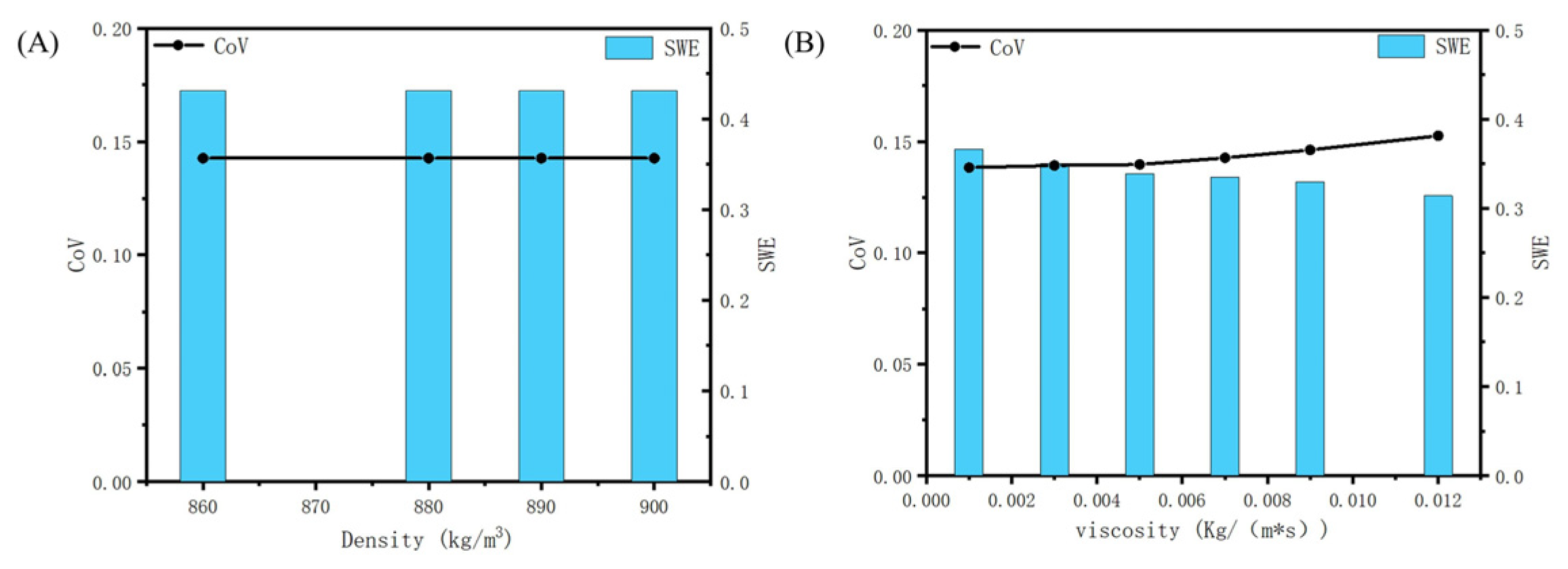
The effects of crude oil density and viscosity on oil–water mixing and salt washing are investigated under the conditions of a crude oil and water flow rate of 2 m/s and an oil–water interfacial tension of 0.01 N/m using an SMX static mixer model with four mixing elements.

3.2.1. Density

The effect of crude oil density on the mixing efficiency is shown in Figure 7A and Figure S1. When the type of static mixer, the number of mixing elements, and the interfacial tension between oil and water remain constant, the effect of crude oil density on oil–water mixing and salt washing is minimal.

3.2.2. Viscosity

The effect of viscosity on the oil–water mixing efficiency of the static mixer is shown in Figure 7B and Figure S2. As the viscosity increased, the mixing efficiency decreased. When the viscosity increased from 0.001 kg/(m·s) to 0.012 kg/(m·s), the CoV also increased from 0.1382 to 0.1526. Meanwhile, the viscosity had a more significant effect on the salt washing efficiency. The SWE of 0.3635 was obtained at a viscosity of 0.001 kg/(m·s). As the viscosity increased, the SWE gradually decreased. When the viscosity reached 0.012 kg/(m·s), the SWE decreased to 0.3295. In other words, the higher the viscosity, the worse the oil–water mixing and the salt washing effect.

3.3. Effect of the Water Injection Process

The effects of water injection volume, salt content in water, and oil–water interfacial tension on oil–water mixing and salt washing are investigated using an SMX static mixer model with four mixing elements.

3.3.1. Water Injection Volume

Under the conditions of crude oil density of 880 kg/m³, crude oil viscosity of 0.002 kg/(m·s), and crude oil injection rate of 2 m/s, the effect of washing water volume on oil–water mixing and salt washing is investigated by changing the injection rate of the washing water, as shown in

Table 4. Relationship between wash water injection ratio and injection rate.

Water injection rate (m/s)	0.75	1.25	2	2.5	3
Water–oil ratio (v/v, %)	3.01	5.02	8.03	10.04	12.05

and Figure 8A and Figure S3. This shows that the mixing effect of the static mixer improves slightly as the washing water injection volume increases. At a washing water ratio of 5%, the CoV is 0.1485. When the washing water ratio increased by 12%, the CoV reached 0.1423. Meanwhile, the salt washing effect gradually increased as the washing water injection volume increased. When the injection washing water ratio increased from 3% to 12%, the SWE value for the salt washing effect increased from 0.1916 to 0.4594. However, considering both the treatment effect and the amount of oily wastewater to be treated, the amount of washing water should not be too much, and the process measure of secondary electric desalination washing water reinjection into the first stage is often adopted.

3.3.2. Salt Content in Washing Water

For cost reasons, current electric desalination water injection does not use desalinated water but rather purified water from acidic water stripping units, and it uses a reinjection process. The injected water contains a certain amount of salt [32]. Therefore, it is necessary to investigate the influence of the salt content in the injection water on the salt dissolution effect. The results showed that as the salt concentration in the washing water increased, the salt washing efficiency decreased. The higher the salt content in the washing water, the lower the salt washing efficiency. When the salinity of the washing water is elevated from 0 mg/L to 30 mg/L, there is a reduction in salt washing efficiency by 25%. When the salt concentration in the washing water is 30 mg/L, the salt washing efficiency is 27.06%, which is significantly lower than the salt washing efficiency of 38% in desalinated water. This is because the higher the salt content in the washing water, the greater the decrease in the mass transfer driving force of salt dissolution in the water, which greatly affects the salt washing effect in the static mixer.

3.3.3. Oil–Water Interfacial Tension

Emulsifiers, which are surfactants that lower the interfacial tension between oil and water, are usually added in the electric desalination process to facilitate oil–water mixture. As the typical injection amount of emulsifiers is 5–30 mg/L, they are usually added before the static mixer to disperse and diffuse to the oil–water interface. Therefore, in the Eulerian multiphase flow model, the effect of the type and amount of emulsifier on oil–water mixing and salt washing is simulated by adjusting the interfacial tension between oil and water. The simulation results show that when the oil–water interfacial tensions are 0.005, 0.01, and 0.02 N/m, the salt washing efficiencies are 0.4306, 0.4295, and 0.4251, respectively (Figure 8C and Figure S4). The lower the interfacial tension, the higher the salt washing efficiency. By adjusting the type and dosage of the emulsifier, the oil–water interfacial tension can be controlled below 0.01 N/m, which is beneficial to the salt washing efficiency. Overall, the oil–water interfacial tension has little effect on the oil–water mixing effect and the salt washing efficiency. This is mainly due to the limitations of the Eulerian multiphase flow model in describing the influence of the oil–water interface on the mixing effect at small scales.

3.4. Correlation Analysis of Influencing Factors and Salt Washing Effect and the Salt Washing Efficiency

The bivariate correlations between mixing efficiency and salt washing efficiency and the six types of influencing factors, such as the number of components in the static mixer, crude oils, and water, were analyzed using IBM SPSS Statistics 24 data statistical analysis software, and correlation matrices were obtained (

Table 5. Correlation of factors with SWE.

Relevance	SWE	Number of Mixing Elements	Viscosity of Crude Oil	Density of Crude Oil	Volume of Water Injected	Initial Salt Content of the Injected Water	Oil–Water Interfacial Tension
SWE	1
Number of mixing elements	0.379 *	1
Viscosity of crude oil	−0.092	−0.008	1
Density of crude oil	0.007	0.015	0.002	1
Volume of water injected	0.331 *	−0.018	−0.044	−0.044	1
Initial salt content of the injected water	−0.351 *	0.093	0.013	−0.023	−0.293	1
Oil–water interfacial tension	−0.018	0.071	0.01	−0.018	−0.211	−0.112	1

* indicates relevance.

and

Table 6. Correlation of factors with CoV.

Relevance	CoV	Number of Mixing Elements	Viscosity of Crude Oil	Density of Crude Oil	Volume of Water Injected	Oil–Water Interfacial Tension
CoV	1
Number of mixing elements	−0.973 **	1
Viscosity of crude oil	0.094	−0.008	1
Density of crude oil	−0.02	0.015	0.002	1
Volume of water injected	0.371 *	−0.018	−0.044	−0.044	1
Oil–water interfacial tension	−0.079	0.071	0.01	−0.018	−0.211	1

** indicates significant relevance; * indicates relevance.

). The number of mixing elements in the static mixer and the amount of wash water injected were closely related to the mixing efficiency of the static mixer. Significant correlations were found between the number of mixing elements in the static mixer, the salt content, and the injection volume of the scrubber water and the salt washing effect. Crude oil viscosity and oil–water interfacial tension showed a weak correlation with salt washing and static mixer mixing efficiency. Crude oil density was largely irrelevant to the salt washing and mixing effects.

4. Conclusions

The effects of the static mixer (mixer type and number of mixing elements), crude oil (density and viscosity), and washing water (injection volume, salt content in water, and oil–water interfacial tension) on the oil–water mixing efficiency and the salt washing efficiency were investigated by combining the multiphase flow law and the dissolution dynamics of salts using a Computational Fluid Dynamics (CFD) method. The results show that the mixer type, the number of mixing elements, and the washing water injection volume have a great influence on the oil–water mixing effect.

The number of mixing elements, the salt content in the washing water, and the amount of wash water have a great influence on the salt washing effect. Once a total of four mixing elements is reached, further increases in the number of mixing elements have a minimal effect on the mixing effect and salt washing effect. The efficiency of salt scrubbing is found to decrease by approximately 25% when the concentration of salt in the scrubbing water is increased from 0 mg/L to 30 mg/L. When the amount of water injected into the system is increased from 5% to 8%, the efficiency of salt washing is almost doubled. Consequently, as the amount of water injected continues to increase, the improvement in salt washing efficiency becomes less apparent. The salt washing efficiency can reach 46.3%, and the oil–water mixing effect is also better when the SMX static mixer with four groups of mixing elements is used; the washing water injection volume is 8%, and the oil–water interfacial tension is kept below 0.01 N/m.

References

1. Chen, H. Influences of heavy oil thermal recovery on reservoir properties and countermeasures of Yulou oil bearing sets in Liaohe Basin in China. Arab. J. Geosci. 2019, 12, 363. [Google Scholar] [CrossRef]
2. Kang, W.-L.; Zhou, B.-B.; Issakhov, M.; Gabdullin, M. Advances in enhanced oil recovery technologies for low permeability reservoirs. Pet. Sci. 2022, 19, 1622–1640. [Google Scholar] [CrossRef]
3. Xu, B.; Wang, Y. Profile control performance and field application of preformed particle gel in low-permeability fractured reservoir. J. Pet. Explor. Prod. Technol. 2020, 11, 477–482. [Google Scholar] [CrossRef]
4. Cui, C.; Zhou, Z.; He, Z. Enhance oil recovery in low permeability reservoirs: Optimization and evaluation of ultra-high molecular weight HPAM/phenolic weak gel system. J. Pet. Sci. Eng. 2020, 195, 107908. [Google Scholar] [CrossRef]
5. Yuan, G.; Keane, M.A. Catalyst deactivation during the liquid phase hydrodechlorination of 2,4-dichlorophenol over supported Pd: Influence of the support. Catal. Today 2003, 88, 27–36. [Google Scholar] [CrossRef]
6. Seadat-Talab, M.; Allahkaram, S.R. Failure analysis of overhead flow cooling systems of a light naphtha separator tower at a petrochemical plant. Eng. Fail. Anal. 2013, 27, 130–140. [Google Scholar] [CrossRef]
7. Rikhtehgaran, S.; Wille, L.T. The effect of an electric field on ion separation and water desalination using molecular dynamics simulations. J. Mol. Model 2021, 27, 21. [Google Scholar] [CrossRef] [PubMed]
8. Mortazavi, V.; Moosavi, A.; Nouri-Borujerdi, A. Enhancing water desalination in graphene-based membranes via an oscillating electric field. Desalination 2020, 495, 114672. [Google Scholar] [CrossRef]
9. Sotelo, C.; Favela-Contreras, A.; Sotelo, D.; Beltrán-Carbajal, F.; Cruz, E. Control Structure Design for Crude Oil Quality Improvement in a Dehydration and Desalting Process. Arab. J. Sci. Eng. 2018, 43, 6579–6594. [Google Scholar] [CrossRef]
10. Ye, G.; LÜ, X.; Peng, F.; Han, P.; Shen, X. Pretreatment of Crude Oil by Ultrasonic-electric United Desalting and Dewatering. Chin. J. Chem. Eng. 2008, 16, 564–569. [Google Scholar] [CrossRef]
11. Regner, M.; Östergren, K.; Trägårdh, C. Effects of geometry and flow rate on secondary flow and the mixing process in static mixers—A numerical study. Chem. Eng. Sci. 2006, 61, 6133–6141. [Google Scholar] [CrossRef]
12. Ghanem, A.; Lemenand, T.; Della Valle, D.; Peerhossaini, H. Static mixers: Mechanisms, applications, and characterization methods—A review. Chem. Eng. Res. Des. 2014, 92, 205–228. [Google Scholar] [CrossRef]
13. Hammoudi, M.; Si-Ahmed, E.K.; Legrand, J. Dispersed two-phase flow analysis by pulsed ultrasonic velocimetry in SMX static mixer. Chem. Eng. J. 2012, 191, 463–474. [Google Scholar] [CrossRef]
14. Alhajri, N.A.; White, R.J.; Oshinowo, L.M. High Efficiency Static Mixer Technology for Crude Desalting. In Proceedings of the SPE Kingdom of Saudi Arabia Annual Technical Symposium and Exhibition, Dammam, Saudi Arabia, 23–26 April 2018; p. SPE-192388-MS. [Google Scholar]
15. Wang, C.; Liu, H.; Yang, X.; Wang, R. Research for a Non-Standard Kenics Static Mixer with an Eccentricity Factor. Processes 2021, 9, 1353. [Google Scholar] [CrossRef]
16. Jiang, X.; Xiao, Z.; Jiang, J.; Yang, X.; Wang, R. Effect of element thickness on the pressure drop in the Kenics static mixer. Chem. Eng. J. 2021, 424, 130399. [Google Scholar] [CrossRef]
17. Lowry, E.; Yuan, Y.; Krishnamoorthy, G. A new correlation for single-phase pressure loss through SMV static mixers at high Reynolds numbers. Chem. Eng. Process. Process Intensif. 2022, 171, 108716. [Google Scholar] [CrossRef]
18. Chakleh, R.; Azizi, F. Performance comparison between novel and commercial static mixers under turbulent conditions. Chem. Eng. Process. Process Intensif. 2023, 193, 109559. [Google Scholar] [CrossRef]
19. Moghaddam, S. Effect of Non-Newtonian Fluid on Mixing Quality and Pressure Drop in Several Static Mixers: A Numerical Study. Iran. J. Sci. Technol. Trans. Mech. Eng. 2023, 47, 1585–1597. [Google Scholar] [CrossRef]
20. Liu, Y.; Rao, A.; Ma, F.; Li, X.; Wang, J.; Xiao, Q. Investigation on mixing characteristics of hydrogen and natural gas fuel based on SMX static mixer. Chem. Eng. Res. Des. 2023, 197, 738–749. [Google Scholar] [CrossRef]
21. Zalc, J.M.; Szalai, E.S.; Muzzio, F.J. Mixing dynamics in the SMX static mixer as a function of injection location and flow ratio. Polym. Eng. Sci. 2004, 43, 875–890. [Google Scholar] [CrossRef]
22. Valdes, J.P.; Kahouadji, L.; Liang, F.; Shin, S.; Chergui, J.; Juric, D.; Matar, O.K. On the dispersion dynamics of liquid–liquid surfactant-laden flows in a SMX static mixer. Chem. Eng. J. 2023, 475, 146058. [Google Scholar] [CrossRef]
23. Jegatheeswaran, S.; Ein-Mozaffari, F.; Wu, J. Process intensification in a chaotic SMX static mixer to achieve an energy-efficient mixing operation of non-newtonian fluids. Chem. Eng. Process. Process Intensif. 2018, 124, 1–10. [Google Scholar] [CrossRef]
24. Singh, M.K.; Anderson, P.D.; Meijer, H.E. Understanding and Optimizing the SMX Static Mixer. Macromol. Rapid Commun. 2009, 30, 362–376. [Google Scholar] [CrossRef] [PubMed]
25. Haddadi, M.M.; Hosseini, S.H.; Rashtchian, D.; Ahmadi, G. CFD modeling of immiscible liquids turbulent dispersion in Kenics static mixers: Focusing on droplet behavior. Chin. J. Chem. Eng. 2020, 28, 348–361. [Google Scholar] [CrossRef]
26. Qing, C.L. Calculation and Application of Comprehensive Dissolution Rate of Rock Salt. China Well Rock Salt 1994, 113, 13–14. [Google Scholar]
27. Bouras, H.; Haroun, Y.; Philippe, R.; Augier, F.; Fongarland, P. CFD modeling of mass transfer in Gas-Liquid-Solid catalytic reactors. Chem. Eng. Sci. 2021, 233, 116378. [Google Scholar] [CrossRef]
28. Deising, D.; Marschall, H.; Bothe, D. A unified single-field model framework for Volume-of-Fluid simulations of interfacial species transfer applied to bubbly flows. Chem. Eng. Sci. 2016, 139, 173–195. [Google Scholar] [CrossRef]
29. Haroun, Y.; Legendre, D.; Raynal, L. Volume of fluid method for interfacial reactive mass transfer: Application to stable liquid film. Chem. Eng. Sci. 2010, 65, 2896–2909. [Google Scholar] [CrossRef]
30. Woo, M.; Tischer, S.; Deutschmann, O.; Wörner, M. A step toward the numerical simulation of catalytic hydrogenation of nitrobenzene in Taylor flow at practical conditions. Chem. Eng. Sci. 2021, 230, 116132. [Google Scholar] [CrossRef]
31. Li, H.; Yu, X.; Song, Y.; Li, Q.; Lu, S. Experimental and numerical investigation on optimization of foaming performance of the kenics static mixer in compressed air foam system. Eng. Appl. Comput. Fluid Mech. 2023, 17, 2183260. [Google Scholar] [CrossRef]
32. Patel, C.G.; Barad, D.; Swaminathan, J. Desalination using pressure or electric field? A fundamental comparison of RO and electrodialysis. Desalination 2022, 530, 115620. [Google Scholar] [CrossRef]
Figure 1. Physical modeling of static mixers and single mixing elements (A): SMV static mixer; (B): SSK static mixer; (C): SMX static mixer; (D): schematic diagram of oil and water inlet.
Processes 12 00883 g001
Figure 2. Distribution of oil and water at the outlet. (A) SMV static mixer. (B) SSK static mixer outlet. (C) SMX static mixer.
Processes 12 00883 g002
Figure 3. Various types of static mixer outlet numerical analyses.
Processes 12 00883 g003
Figure 4. Distribution diagram of various types of static mixer pressures. (A) SMV static mixer pressure distribution. (B) SSK static mixer pressure distribution. (C) SMX static mixer pressure distribution diagram.
Processes 12 00883 g004
Figure 5. Physical modelling of the static mixer and simulation of oil–water separation at the outlet. (A) Schematic diagram of a single mixing element. (B) Schematic diagram of double mixing elements. (C) Schematic diagram of triple mixing elements. (D) Schematic diagram of quadruple mixing elements. (E) Schematic diagram of quintuple mixing elements. (F) Distribution of oil fractions exported from a single mixing element. (G) Distribution of oil fractions exported from double mixing elements. (H) Distribution of oil fractions exported from triple mixing elements. (I) Distribution of oil fractions exported from quadruple mixing elements. (J) Distribution of oil fractions exported from quintuple mixing elements.
Processes 12 00883 g005
Figure 6. Results for different numbers of mixing elements. (A) Effect on CoV. (B) Effect on SWE. (C) Effect on differential pressure.
Processes 12 00883 g006
Figure 7. Effect of oil properties on results. (A) Oil density. (B) Oil viscosity.
Processes 12 00883 g007
Figure 8. Effect of water injection on results. (A) Water injection volume. (B) Salt content in washing water. (C) Oil–water interfacial tension.
Processes 12 00883 g008