Reduced Models in Chemical Kinetics via Nonlinear Data-Mining

 ,
,
Abstract
:1. Introduction
2. Diffusion Maps

2.1. Issues in the Implementation of the Algorithm

3. The Proposed Approach
3.1. Data Collection

- Compute the y on corresponding to the current u (using whatever form of interpolation we chose earlier);
- Compute ;
- Compute the equivalent .
3.2. Interpolation/Extension Schemes
3.2.1. Nyström Extension
3.2.2. Radial Basis Functions
3.2.3. Kriging
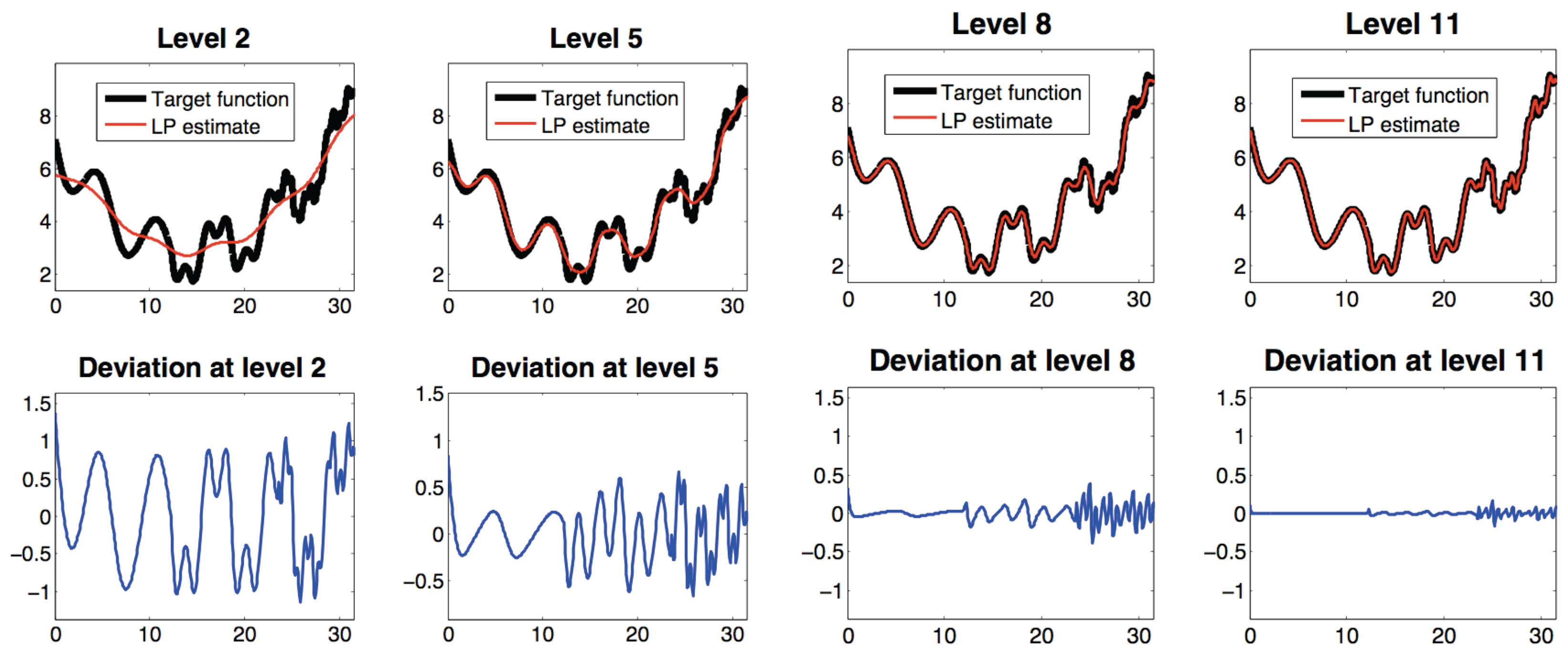
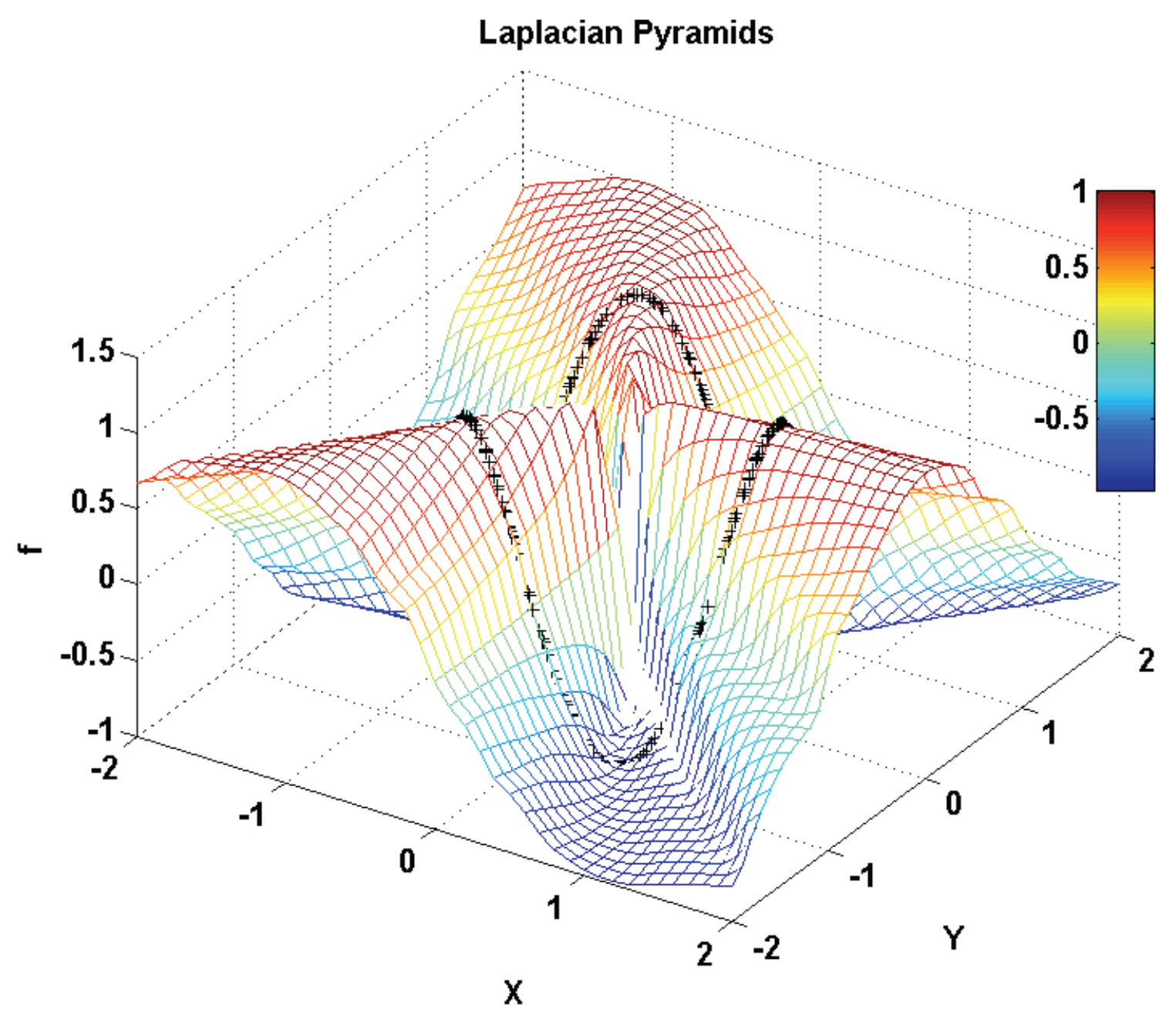
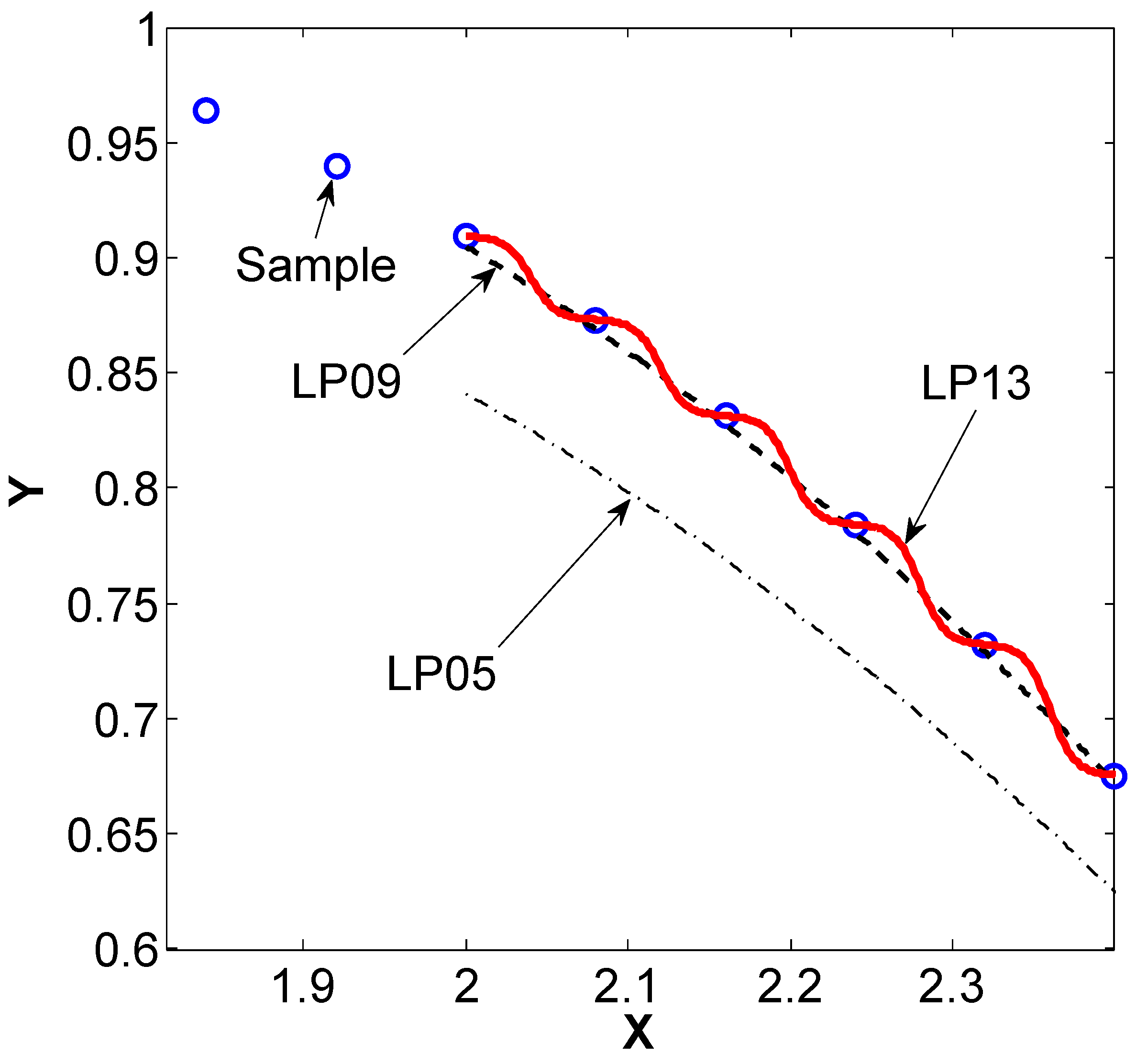
3.2.4. Laplacian Pyramids

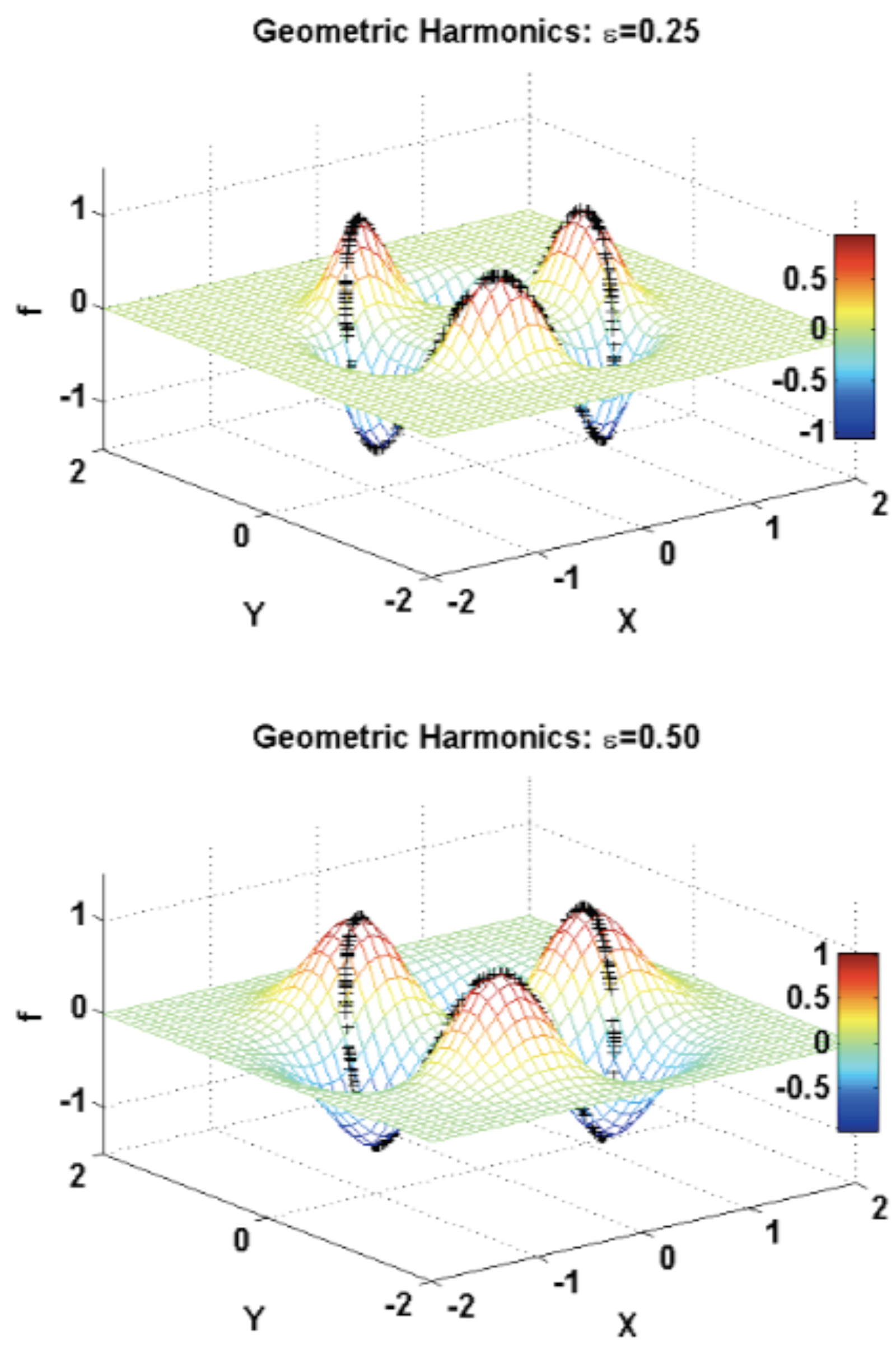
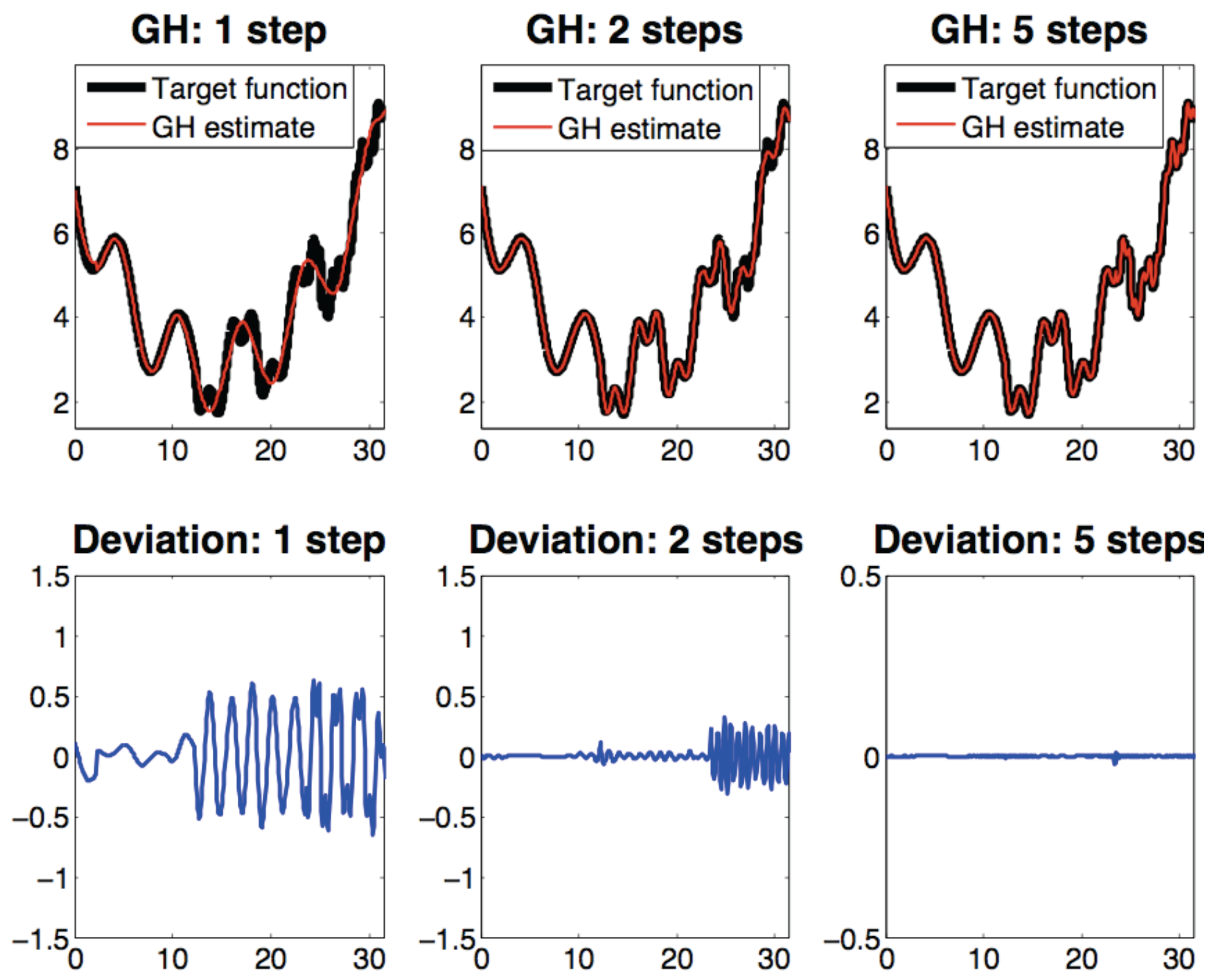
3.2.5. Geometric Harmonics

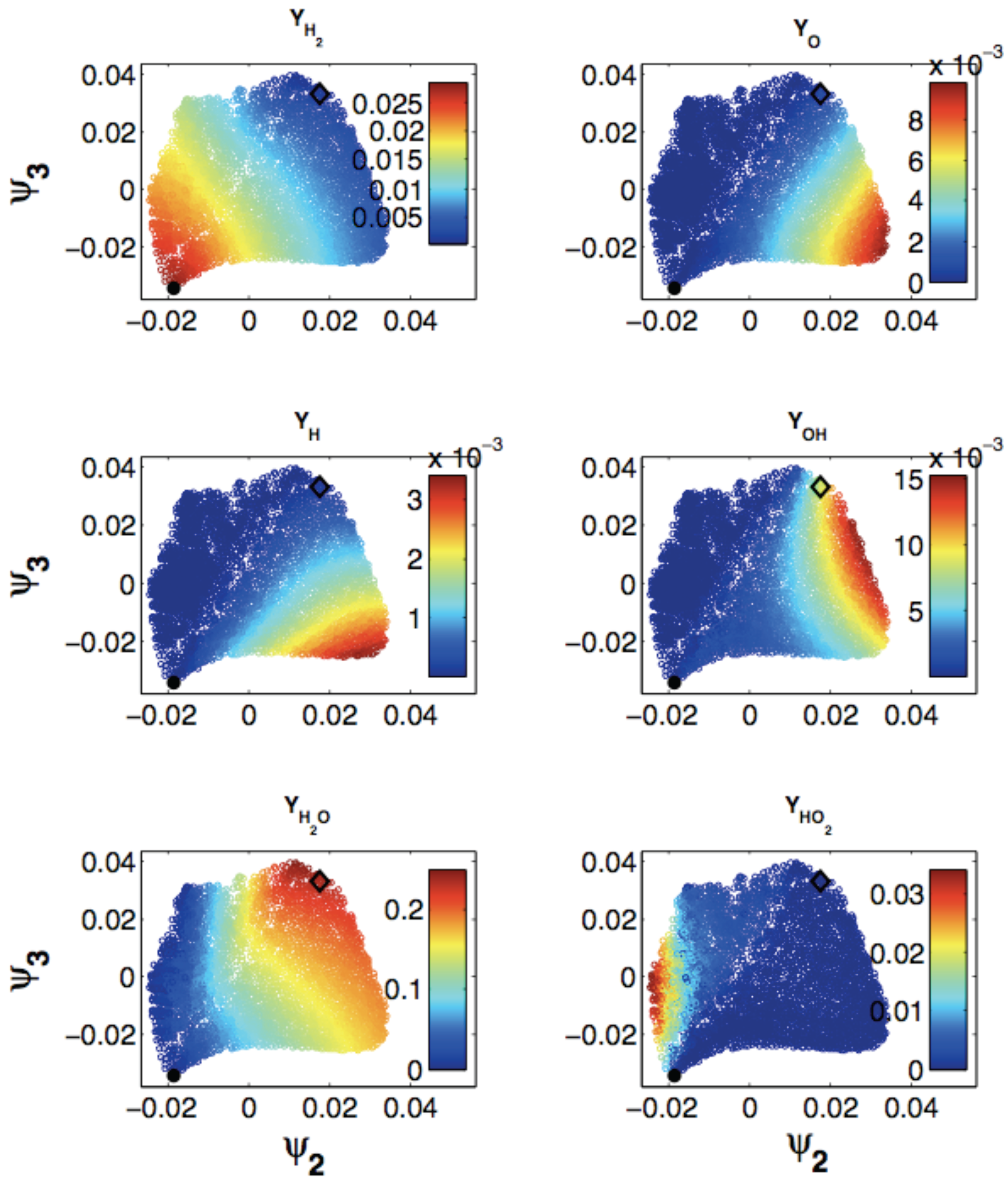
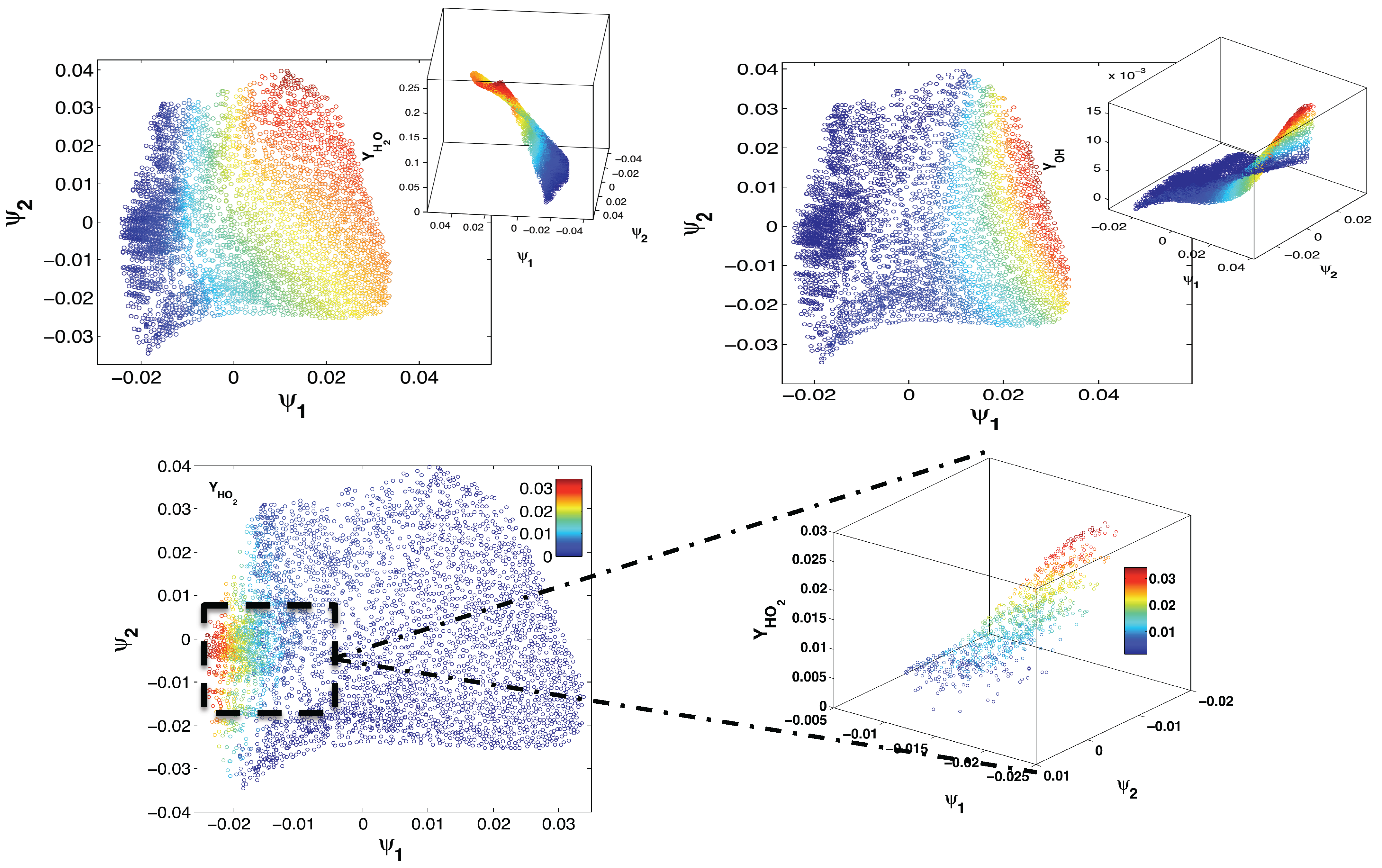
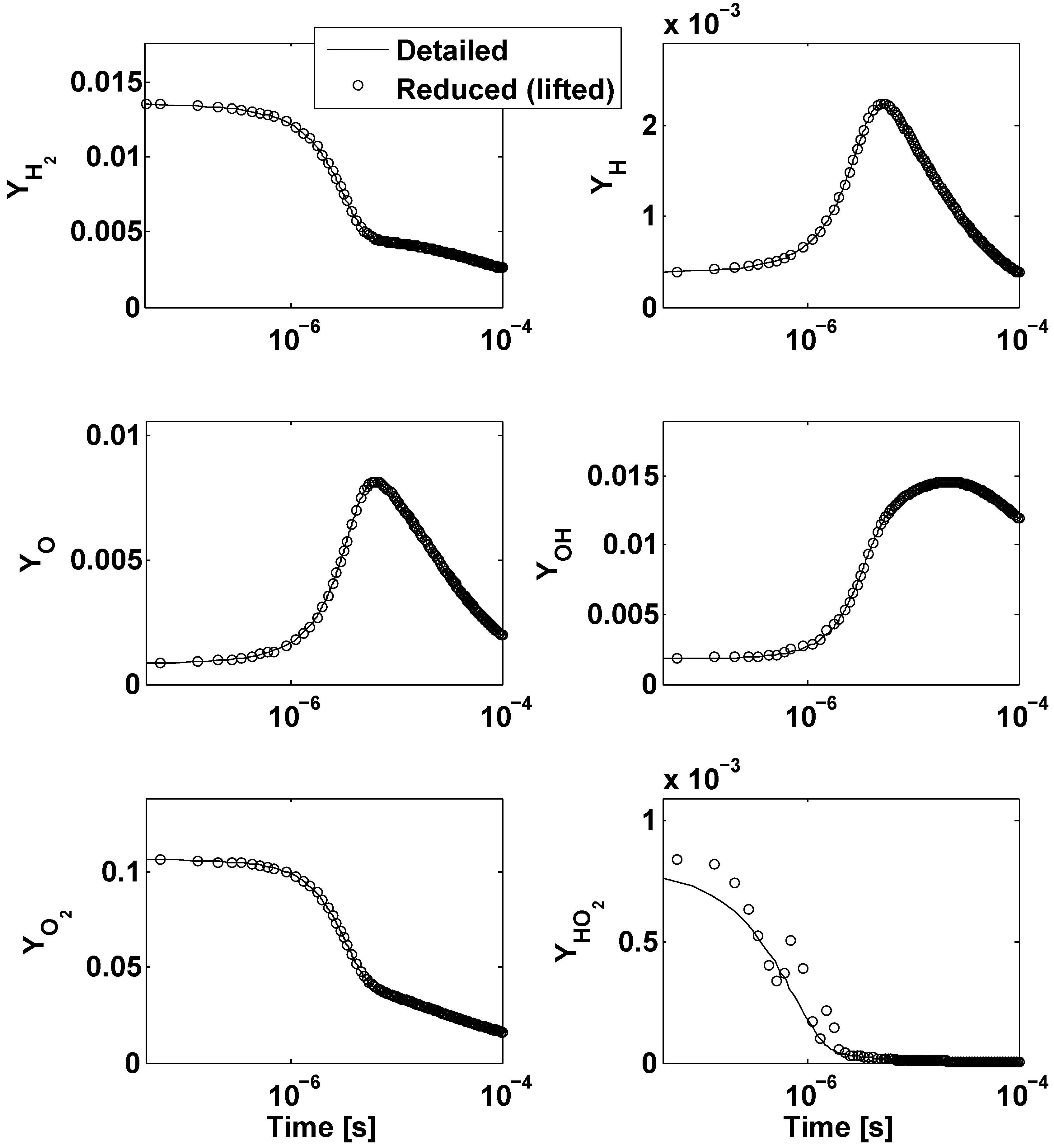
4. Application to an Illustrative Example: Homogeneous Combustion


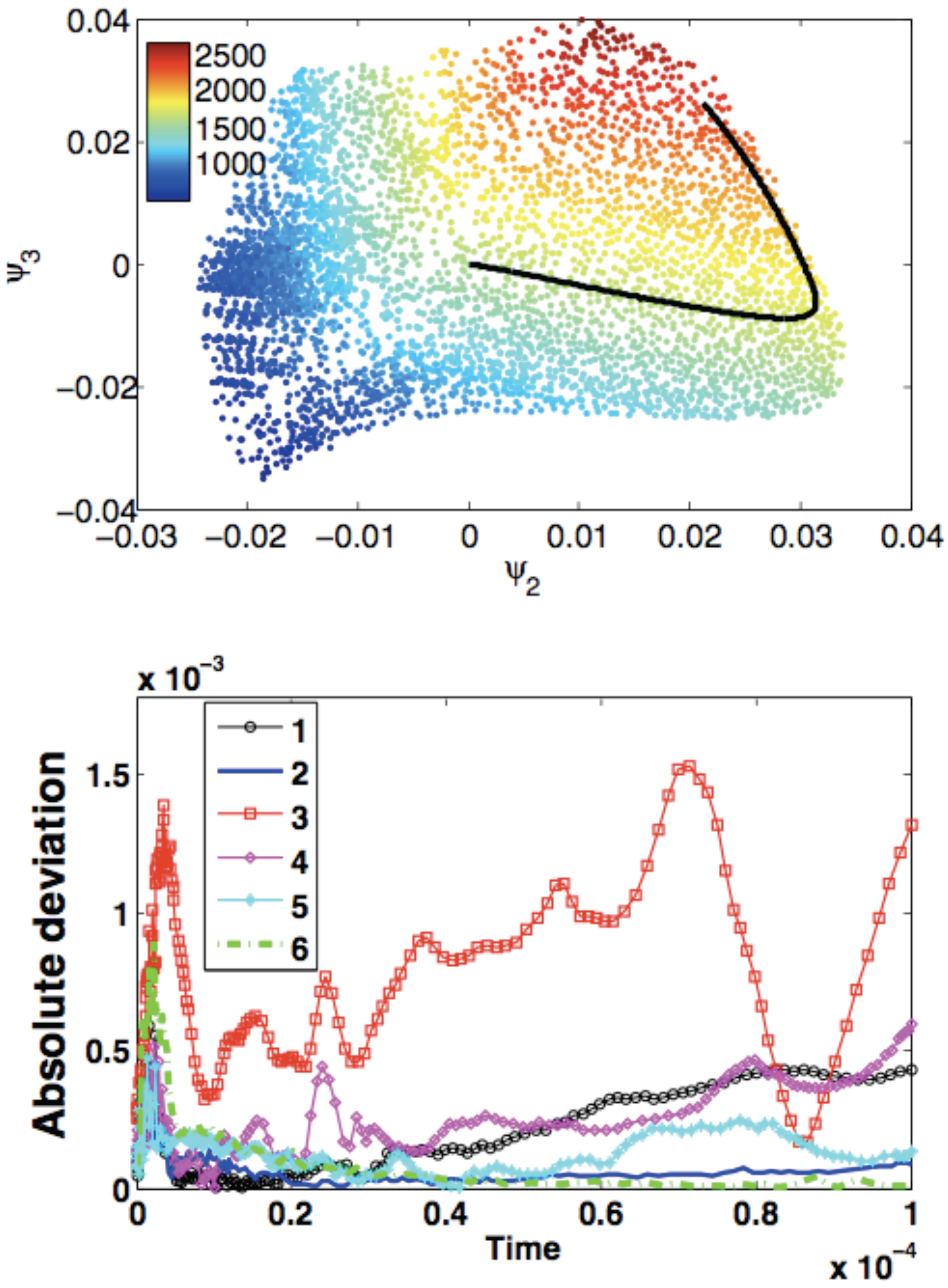
| Method | |||||||||
|---|---|---|---|---|---|---|---|---|---|
| 1 | |||||||||
| 2 | |||||||||
| 3 | |||||||||
| 4 | |||||||||
| 5 | |||||||||
| 6 | |||||||||
| 7 | |||||||||
| 8 | |||||||||
| 9 | |||||||||
| 10 | |||||||||
| 11 | |||||||||
| 12 |
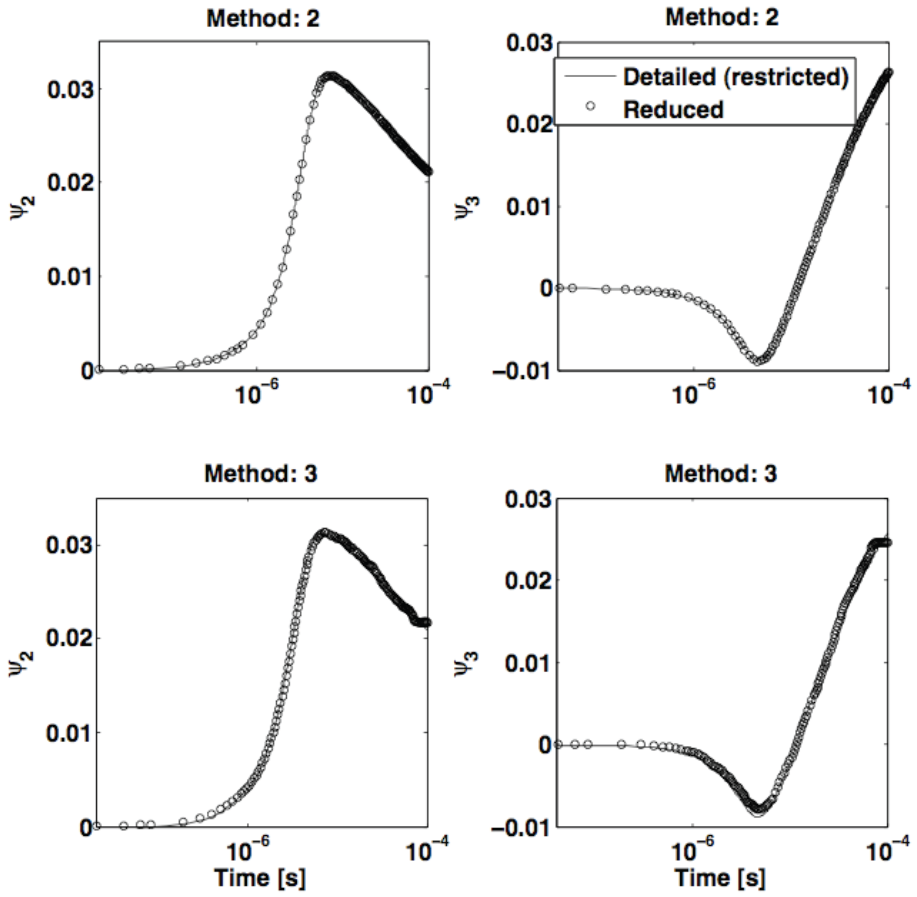
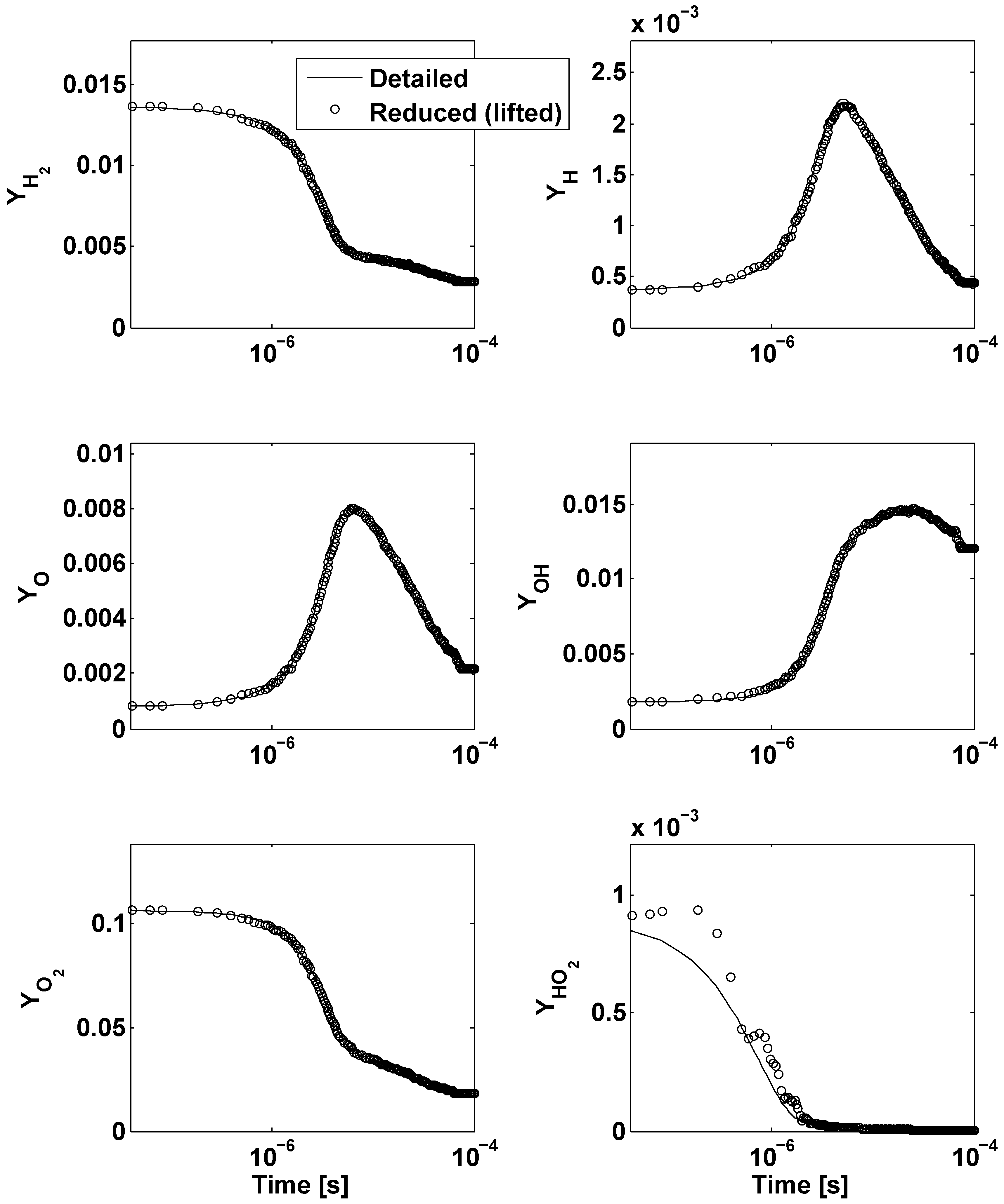
- The lifting operator consists of radial basis function interpolation with performed over 50 nearest neighbors of an arbitrary point in the reduced space, u. Restriction is done by radial basis function interpolation with performed over 50 nearest neighbors of an arbitrary point in the ambient space, y. The reduced dynamical system is expressed in the form of Equation (13).
- The lifting operator consists of radial basis function interpolation with performed over 50 nearest neighbors of an arbitrary point in the reduced space, u. Restriction is done by the Nyström method. The reduced dynamical system is expressed in the form of Equation (13).
- The lifting operator is based on Laplacian Pyramids up to a level with over 80 nearest neighbors of an arbitrary point in the reduced space, u. Restriction is based on the Laplacian Pyramids up to a level with over 80 nearest neighbors of y. The reduced dynamical system is expressed in the form of Equation (13).
- The lifting operator is based on Laplacian Pyramids up to a level with . Restriction is done by the Nyström method. The reduced dynamical system is expressed in the form of Equation (13).
- The lifting operator is based on Geometric Harmonics locally performed over 15 nearest neighbors of an arbitrary point in the reduced space, u. Refinements are performed until the Euclidean norm of the residual is larger than . Restriction is done by the Nyström method. The reduced dynamical system is expressed in the form of Equation (13).
- The lifting operator is based on Kriging performed over eight nearest neighbors of an arbitrary point in the reduced space, u (DACE package [27], with a second order polynomial regression model, a Gaussian correlation model and parameter ). Restriction is done by the Nyström method. The reduced dynamical system is expressed in the form of Equation (13).
- The lifting operator is based on Geometric Harmonics locally performed over 10 nearest neighbors of an arbitrary point in the reduced space, u. Refinements are performed until the Euclidean norm of the residual is larger than . Restriction is done using the Nyström method. The reduced dynamical system is expressed in the form of Equation (13).
- The lifting operator is based on Kriging performed over eight nearest neighbors of an arbitrary point in the reduced space, u (DACE package [27], with a second order polynomial regression model, a Gaussian correlation model and parameter ). Restriction is done by the Nyström method. The reduced dynamical system is expressed in the form of Equation (14).
- The lifting operator is based on Kriging performed globally over all samples (package [27], with a second order polynomial regression model, a Gaussian correlation model and parameter ). Restriction is done by the Nyström method. The reduced dynamical system is expressed in the form of Equation (14).
- The lifting operator is based on the Laplacian Pyramids up to a level with over 80 nearest neighbors of an arbitrary point in the reduced space, u. Restriction is based on the Laplacian Pyramids up to a level with over 80 nearest neighbors of an arbitrary point in the ambient space, y. The reduced dynamical system is expressed in the form of Equation (13).
- The lifting operator is based on the Laplacian Pyramids up to a level with over 80 nearest neighbors of an arbitrary point in the reduced space, u. Restriction is based on the Laplacian Pyramids up to a level with over 80 nearest neighbors of an arbitrary point in the ambient space, y. The reduced dynamical system is expressed in the form of Equation (13).
- The lifting operator is based on the Laplacian Pyramids up to a level with over 80 nearest neighbors of an arbitrary point in the reduced space, u. Restriction is based on Laplacian Pyramids up to a level with over 80 nearest neighbors of an arbitrary point in the ambient space, y. The reduced dynamical system is expressed in the form of Equation (13).

5. Conclusions
Acknowledgments
Conflicts of Interest
References
- Maas, U.; Goussis, D. Model Reduction for Combustion Chemistry. In Turbulent Combustion Modeling; Echekki, T., Mastorakos, E., Eds.; Springer: New York, NY, USA, 2011; pp. 193–220. [Google Scholar]
- Chiavazzo, E.; Karlin, I.V.; Gorban, A.N.; Boulouchos, K. Coupling of the model reduction technique with the lattice Boltzmann method for combustion simulations. Combust Flame 2010, 157, 1833–1849. [Google Scholar] [CrossRef]
- Ren, Z.; Pope, S.B.; Vladimirsky, A.; Guckenheimer, J.M. The invariant constrained equilibrium edge preimage curve method for the dimension reduction of chemical kinetics. J. Chem. Phys. 2006, 124, 114111. [Google Scholar] [CrossRef] [PubMed]
- Chiavazzo, E.; Karlin, I.V. Adaptive simplification of complex multiscale systems. Phys. Rev. E 2011, 83, 036706. [Google Scholar] [CrossRef]
- Chiavazzo, E. Approximation of slow and fast dynamics in multiscale dynamical systems by the linearized Relaxation Redistribution Method. J. Comp. Phys. 2012, 231, 1751–1765. [Google Scholar] [CrossRef]
- Pope, S.B. Computationally efficient implementation of combustion chemistry using in situ adaptive tabulation. Combust Theory Model 1997, 1, 41–63. [Google Scholar]
- Coifman, R.R.; Lafon, S.; Lee, A.B.; Maggioni, M.; Nadler, B.; Warner, F.; Zucker, S.W. Geometric diffusions as a tool for harmonic analysis and structure definition of data: Diffusion maps. Proc. Natl. Acad. Sci. USA 2005, 102, 7426–7431. [Google Scholar] [CrossRef] [PubMed]
- Coifman, R.R.; Lafon, S.; Lee, A.B.; Maggioni, M.; Nadler, B.; Warner, F.; Zucker, S.W. Geometric diffusions as a tool for harmonic analysis and structure definition of data: Multiscale methods. Proc. Natl. Acad. Sci. USA 2005, 102, 7432–7437. [Google Scholar] [CrossRef] [PubMed]
- Coifman, R.R.; Lafon, S. Diffusion maps. Appl. Comput. Harmon. Anal. 2006, 21, 5–30. [Google Scholar] [CrossRef]
- Jolliffe, I.T. Principal Component Analysis; Springer-Verlag: New York, NY, USA, 2002. [Google Scholar]
- Jones, P.W.; Maggioni, M.; Schul, R. Manifold parametrizations by eigenfunctions of the laplacian and heat kernels. Proc. Nat. Acad. Sci. USA 2008, 105, 1803–1808. [Google Scholar] [CrossRef]
- Lafon, S. Diffusion Maps and Geometric Harmonics. Ph.D. Thesis, Yale University, New Haven, CT, USA, 2004. [Google Scholar]
- Grassberger, P. On the Hausdorff dimension of fractal attractors. J. Stat. Phys. 1981, 26, 173–179. [Google Scholar] [CrossRef]
- Grassberger, P.; Procaccia, I. Measuring the strangeness of strange attractors. Physica D 1983, 9, 189–208. [Google Scholar] [CrossRef]
- Coifman, R.R.; Shkolnisky, Y.; Sigworth, F.J.; Singer, A. Graph laplacian tomography from unknown random projections. IEEE Trans. Image Process. 2008, 17, 1891–1899. [Google Scholar] [CrossRef] [PubMed]
- Maas, U.; Pope, S. Simplifying chemical kinetics: Intrinsic low-dimensional manifolds in composition space. Combust Flame 1992, 88, 239–264. [Google Scholar] [CrossRef]
- Kevrekidis, I.G.; Gear, C.W.; Hyman, J.M.; Kevrekidis, P.G.; Runborg, O.; Theodoropoulos, C. Equation-free, coarse-grained multiscale computation: Enabling mocroscopic simulators to perform system-level analysis. Comm. Math. Sci. 2003, 1, 715–762. [Google Scholar]
- Kevrekidis, I.G.; Gear, C.W.; Hummer, G. Equation-free: The computer-aided analysis of complex multiscale systems. AIChE J. 2004, 50, 1346–1355. [Google Scholar] [CrossRef]
- Kroese, D.P.; Taimre, T.; Botev, Z.I. Handbook of Monte Carlo Methods; Wiley: Hoboken, NJ, USA, 2011. [Google Scholar]
- Kaufman, D.E.; Smith, R.L. Direction choice for accelerated convergence in hit-and-run sampling. Oper. Res. 1998, 46, 84–95. [Google Scholar] [CrossRef]
- Gear, C.W. Parameterization of Non-Linear Manifolds. Available online: http://www.princeton.edu/wgear/ (accessed on 23 September 2013).
- Sonday, B.E.; Gear, C.W.; Singer, A.; Kevrekidis, I.G. Solving differential equations by model reduction on learned manifolds. Unpublished. 2011. [Google Scholar]
- Rohrdanz, M.A.; Zheng, W.; Maggioni, M.; Clementi, C. Determination of reaction coordinates via locally scaled disffusion map. J. Chem. Phys. 2011, 134, 124116. [Google Scholar] [CrossRef]
- Nyström, E.J. Über die praktische Auflösung von linearen integralgleichungen mit anwendungen auf randwertaufgaben der potentialtheorie. Commentationes Physico-Mathematicae 1928, 4, 1–52. (in German). [Google Scholar]
- Sonday, B.E. Systematic Model Reduction for Complex Systems through Data Mining and Dimensionality Reduction. Ph.D. Thesis, Princeton University, Princeton, NJ, USA, 2011. [Google Scholar]
- Isaaks, E.H.; Srivastava, R.M. An Introduction to Applied Geostatistics; Oxford University Press: New York, NY, USA, 1989. [Google Scholar]
- Lophaven, S.N.; Nielsen, H.B.; Søndergaard, J. DACE A Matlab Kriging Toolbox. In Technical Report IMM-TR-2002-12; Technical University of Denmark: Kongens Lyngby, Denmark, 2002; pp. 1–26. [Google Scholar]
- Rabin, N.; Coifman, R.R. Heterogeneous Datasets Representation and Learning Using Diffusion Maps and Laplacian Pyramids. In Proceedings of the 12th SIAM International Conference on Data Mining, Anaheim, CA, USA, 26–28 August 2012; pp. 189–199.
- Coifman, R.R.; Lafon, S. Geometric harmonics: A novel tool for multiscale out-of-sample extension of empirical functions. Appl. Comput. Harmon. Anal. 2006, 21, 31–52. [Google Scholar] [CrossRef]
- Li, J.; Zhao, Z.; Kazakov, A.; Dryer, F.L. An updated comprehensive kinetic model of hydrogen combustion. Int. J. Chem. Kinet. 2004, 36, 566–575. [Google Scholar] [CrossRef]
- Frewen, T.A.; Hummer, G.; Kevrekidis, I.G. Exploration of effective potential landscapes using coarse reverse integration. J. Chem. Phys. 2009, 131, 134104. [Google Scholar] [CrossRef] [PubMed]
- Dsilva, C.J.; Talmon, R.; Rabin, N.; Coifman, R.R.; Kevrekidis, I.G. Nonlinear intinsic variables and state reconstruction in multiscale simulations. J. Chem. Phys. 2013, 139, 184109. [Google Scholar] [CrossRef] [PubMed]
© 2014 by the authors; licensee MDPI, Basel, Switzerland. This article is an open access article distributed under the terms and conditions of the Creative Commons Attribution license (http://creativecommons.org/licenses/by/3.0/).
Share and Cite
Chiavazzo, E.; Gear, C.W.; Dsilva, C.J.; Rabin, N.; Kevrekidis, I.G. Reduced Models in Chemical Kinetics via Nonlinear Data-Mining. Processes 2014, 2, 112-140. https://doi.org/10.3390/pr2010112
Chiavazzo E, Gear CW, Dsilva CJ, Rabin N, Kevrekidis IG. Reduced Models in Chemical Kinetics via Nonlinear Data-Mining. Processes. 2014; 2(1):112-140. https://doi.org/10.3390/pr2010112
Chicago/Turabian StyleChiavazzo, Eliodoro, Charles W. Gear, Carmeline J. Dsilva, Neta Rabin, and Ioannis G. Kevrekidis. 2014. "Reduced Models in Chemical Kinetics via Nonlinear Data-Mining" Processes 2, no. 1: 112-140. https://doi.org/10.3390/pr2010112