Article

Life Cycle Network Modeling Framework and Solution Algorithms for Systems Analysis and Optimization of the Water-Energy Nexus

Department of Chemical and Biological Engineering, Northwestern University, 2145 Sheridan Road, Evanston, IL 60208
*
Author to whom correspondence should be addressed.
Processes 2015, 3(3), 514-539; https://doi.org/10.3390/pr3030514
Submission received: 29 April 2015 / Accepted: 6 July 2015 / Published: 13 July 2015
(This article belongs to the Special Issue Sustainable Products and Processes)

Abstract

:
The water footprint of energy systems must be considered, as future water scarcity has been identified as a major concern. This work presents a general life cycle network modeling and optimization framework for energy-based products and processes using a functional unit of liters of water consumed in the processing pathway. We analyze and optimize the water-energy nexus over the objectives of water footprint minimization, maximization of economic output per liter of water consumed (economic efficiency of water), and maximization of energy output per liter of water consumed (energy efficiency of water). A mixed integer, multiobjective nonlinear fractional programming (MINLFP) model is formulated. A mixed integer linear programing (MILP)-based branch and refine algorithm that incorporates both the parametric algorithm and nonlinear programming (NLP) subproblems is developed to boost solving efficiency. A case study in bioenergy is presented, and the water footprint is considered from biomass cultivation to biofuel production, providing a novel perspective into the consumption of water throughout the value chain. The case study, optimized successively over the three aforementioned objectives, utilizes a variety of candidate biomass feedstocks to meet primary fuel products demand (ethanol, diesel, and gasoline). A minimum water footprint of 55.1 ML/year was found, economic efficiencies of water range from −$1.31/L to $0.76/L, and energy efficiencies of water ranged from 15.32 MJ/L to 27.98 MJ/L. These results show optimization provides avenues for process improvement, as reported values for the energy efficiency of bioethanol range from 0.62 MJ/L to 3.18 MJ/L. Furthermore, the proposed solution approach was shown to be an order of magnitude more efficient than directly solving the original MINLFP problem with general purpose solvers.

Graphical Abstract

1. Introduction

Sustainability is a key area of interest in both academia and industry. This state of affairs has not always been the case, especially in the industrial sector, and its recent emergence has guided thought and galvanized efforts to understand, quantify, and optimize sustainability indicators in an industrial context [1,2]. The concept of the water footprint has recently been identified as a key environmental indicator of sustainability [3]. Fresh water is expected to be a scarce commodity in the future in many areas of the world [3]. Indeed, the western portion of the United States has seen unprecedented drought in recent years, placing increasing stress on that region’s agricultural economy [4]. As the world becomes more populous and its people richer (and more likely to increase water consumption per capita), water must be treated as a precious resource. Energy and industrial sectors consume large quantities of water, and some key work has been performed to understand the water footprint of this sector [5,6,7]. For example, the process systems engineering community has played a key role in characterizing and optimizing water recycling and minimization [5,6,7].
However, one of the major consumers of fresh water in the United States is the energy sector, with approximately 40% of all fresh water withdrawals directed towards meeting cooling demand for electricity production [8]. Energy and water are closely intertwined, leading to the concept of the water-energy nexus [9,10,11,12]. Indeed, water has been a source of energy and productivity throughout history, from watermills to the hydroelectric dams of today that generate 19% of the world’s electricity [13]. While hydroelectric dams have clear connections to the water-energy nexus and have been the subject of key studies to determine their water footprints [14], most water consumption in the energy sector is used for cooling demands of power plants. Thus, regardless of how the energy is generated, if fresh water resources are expected to become scarce, all sectors of the energy industry will be exposed. While water networks themselves have been the subject of energy and mass exchange studies [15], it is critical to thoroughly understand the influences water and energy have on each other and their connections to each other in the water-energy nexus.
Several studies have quantified and optimized the water-energy nexus of energy systems. Gao et al. optimized the water-energy nexus of shale gas production [16]. Murphy and Allen found that the water footprint of biodiesel production from microalgae was extremely high [17]. Manufacturing industries use a large amount of water for energy in the form of steam, and this aspect of the water-energy nexus was recently explored by Walker et al. [18]. They found that the fresh water footprint of the U.S. manufacturing sector was as large as that of the city of Los Angeles, highlighting the importance of and potential for water footprint minimization in energy applications. Many studies have optimized energy consumption and the water footprint of other energy applications, including in corn ethanol plants [19], thermochemical hybrid biomass, coal, and natural gas facilities [20], and batch process scheduling operations [21]. However, the water-energy nexus of biofuels and bioenergy systems has received less attention. This topic is extremely important [22,23], as biomass cultivation and agriculture can consume vast quantities of water. Furthermore, biofuels are a critical component of the food-water-energy nexus, and this property has galvanized the development of multiobjective models for optimal consumption of different types of biomass [24]. Initial work focused on the water-energy nexus found that optimizing the energy consumption of a bioethanol facility in turn reduces the amount of makeup fresh water required for heating and cooling [25]. An energy, water, and process integration study was performed for conversion of both corn and corn stover to ethanol [26]. Ahmetović et al. optimized energy and water consumption of a corn grain to ethanol facility [19]. These studies found that recycling of water streams and minimizing energy consumption were critical to reducing the water footprint of bioconversion technologies that utilize corn or corn stover feedstocks. However, many more potential technologies are available today that can use alternative feedstocks such as switchgrass, woody biomass, and algae. Indeed, Kantas et al. found that using switchgrass to produce ethanol was a profitable and environmentally preferable process with an abundance of available biomass [27]. It will be key to quantify, understand, and optimize the water-energy nexus of all proposed biofuels technologies to ensure sustainable development in this space.
This work aims to provide a new product and process network-focused water-energy nexus optimization strategy. This task is accomplished first by building a comprehensive process and product network model that can account for both the economics and water footprints of each technology and throughout the processing pathways. This model is the first product and process network model to account for water consumption data taken from technoeconomic analyses and other literature sources to estimate the water footprint of the final processing pathway. Life cycle optimization [28,29,30,31,32] is then incorporated by introducing a functional unit of “liters of water consumed” to determine optimal processing pathways. In addition to an objective of minimizing the overall water footprint, this functional unit is integrated with the economic and energy outputs of the processing pathway to create novel objectives of the economic efficiency of water and the energy efficiency of water. Both objectives are to be maximized. A multiobjective mixed integer nonlinear fractional programming (MINLFP) model is constructed. A novel solution method that employs a mixed integer linear programming (MILP) based branch and refine algorithm using piecewise linear approximations, nonlinear programming subproblems, and the parametric algorithm is developed. This solution method could reduce the computational complexity of the original problem and could boost computational solving efficiency. With this new network-based optimization tool and novel solution method, the three aforementioned objectives are used in a bioconversion process and product network case study. The construction of the network model and its formulation is described in the following section, followed by a discussion of the results.

2. Approach

2.1. Data Collection and Life Cycle Optimization Approach

Much of the data collection strategy can be found in the author’s previous work, including methods for extracting reference operating costs, capital costs, yields, and energy use [33]. Similar methods are employed to extract water consumption rate data corresponding to each technology’s reference capacity. Extracting water consumption data directly from the literature for the purpose of optimization could provide a novel, concrete lens with which to optimize processing pathways. The reference capacities and corresponding data were retrieved from a variety of sources including technoeconomic analyses and journal articles. While the data included in this particular work is derived from bioconversion process and product technologies, the overall data collection, modeling, and solution strategies presented here hold for a variety of energy-focused process and product networks. Only data from relatively advanced technologies were included in the model; no data collected from investigations at the lab-scale or smaller were included.
Both indirect and direct process water consumption was retrieved from technoeconomic analyses and design reports (for example, [34,35,36]). Most direct water consumption (e.g., water used for reactions) data were retrieved from analyzing mass flow streams. When direct water consumption was not explicitly provided, the amount of makeup water needed in the process models was used. Indirect water consumption via cooling and heating was taken into account.
Key considerations of life cycle analysis (LCA) and life cycle optimization include a well-defined system boundary and functional unit [37]. In this work, we consider a system boundary of “cradle to gate.” Thus, water footprints, costs, revenues, and energy production rates are considered in production of inputs, transportation of inputs, processing, and production of the final products. Water is consumed throughout the pathway, with negligible consumption assumed during transportation of processing inputs and raw materials. The final energy products are assumed to be the only sources of output energy from the system boundary (i.e., no raw materials or inputs undergo direct combustion for heat or power). A functional unit of “liters of water consumed” is chosen to better understand the interactions between the water footprint and energy production throughout the processing pathway. Using this functional unit, we can define three different, key objectives to optimize an energy process and product network in a multiobjective study. One objective is the minimization of the water footprint. Next, we integrate the functional unit with an economic indicator—the net present value (NPV)—to form an objective to maximize the NPV per amount of water consumed. We refer to this quantity as the economic efficiency of water in reference to previous works, where it was presented as a “broader concept, seeking the highest economic value of water use through both physical and managerial issues” [38]. Conceptually, this quantity allows for the maximization of the economic value that the processing pathway can produce for each liter of input water. Thus, using the economic efficiency of water as an objective inherently accounts for the tradeoff between processing pathways with low costs but high water footprints and processing pathways with high costs but low water footprints. Finally, the functional unit of liters of water consumed can be integrated with the amount of energy produced to develop an objective of the energy efficiency of water, i.e., how much usable energy in the form of final products is produced per liter of water consumed. The life cycle boundary, functional unit definition, and objective functions can be used for any general energy-based product and process network, as long as appropriate data is collected.

2.2. Model Formulation

This section details the construction of the multiobjective optimization model used to identify optimal processing pathways from a product and process network. A focus is placed on modeling and optimizing the water-energy nexus of this network: the economic and energy efficiencies of water are both taken into account. The model is general in that it can be applied to a wide variety of product and process networks. Thus, while this work focuses on the specific case of a bioconversion product and process network, the model formulation and solution methods described here are general. Variables are denoted in upper case, and parameters are denoted in lowercase.

2.2.1. Sets and Notation

This section will discuss the sets and subsets used in the following model formulation. The set iєI represents all compounds and materials in the model. The subset BϵI represents the feedstocks or raw materials, and the subset FϵI represents the fuels products. The set jєJ represents all technologies in the model. Parameters that reflect data inputs are indicated in lowercase. All decision variables are written in uppercase. A full list of parameters and variables can be found in the Appendix.

2.2.2. Objective Functions

Three objectives are investigated in this work. One objective is to minimize the life cycle blue water footprint of the processing pathway:
OBJ water = W F
where WF is a variable for the processing pathway’s water footprint, measured in liters of water per year. In a bioconversion example, water can be consumed during biomass cultivation and in the processing pathway. The energy efficiency of water for the processing pathway can also be maximized:
OBJ EEW = F E W F
where FE is the energy available in the final set of fuels or other energy products produced from the processing pathway. As mentioned in the previous section, this quantity, the energy efficiency of energy, conceptually represents the amount of usable energy in the form of final products to be produced per liter of water consumed. Finally, the economic efficiency of water can be maximized:
OBJ EcEW = N P V W F
where NPV is the net present value of the processing pathway. To reiterate, the economic efficiency of water reflects the economic value (cost) produced (required) for each liter of water consumed throughout the processing pathway.
In addition to the objective functions outlined above, economic, mass balance, and water constraints are to be added to the model, summarized in the following subsections.

2.2.3. Economic Constraints

The NPV of the processing pathway takes into account revenues and costs:
N P V = i F S i s p i ( j ( f c f j + c c h f ) C C j + X j r e f c j r e f o c j + i B P i ( f p i + v t c i + f t c i ) + e c j u e j X j )
where fcfj is the fixed cost factor for technology j, cchf is the capital charge factor required to annualize the capital cost for appropriate calculation of the NPV, CCj is the capital cost of technology j, Xj is the capacity of technology j, refcj is the reference capacity for technology j, refocj is the reference operating cost for technology j, Pi is the quantity purchased of material/compound i, fpi is the feedstock price of compound i, vtci is the variable transportation cost of feedstock i, ftci is the fixed transportation cost of feedstock i, ec is the cost of electricity, uej is the unit energy consumption of technology j, Si is the quantity sold of final product i, and spi is the selling price of final product i. We note that the fixed transportation cost term ftci is in distance-fixed units of $/kg, so it must be multiplied by the quantity purchased Pi. Similarly, the variable transportation costs are variable costs that change based on the distance traveled. The transportation distance has been assumed to be pre-determined by the user and is already incorporated into each parameter ftci and vtci. The capital charge factor cchfi can be calculated from an interest rate r and anticipated processing pathway lifetime n:
c c h f = ( r ( 1 + r ) n ( 1 + r ) n 1 )
The capital cost for each technology in the pathway can be calculated as follows:
C C j = r e f c c j c c f X j s f j , j
where refccj is the reference capital cost of technology j corresponding to refcj, sfj is the scaling factor for capital cost with capacity, and ccf is the capital cost factor that takes into account the chemical engineering plant cost index (CEPCI) from the year the technology was reported to the current year.
In the case of large scale energy developments, capital costs are always a concern. For example, a recently constructed biofuels plant in Iowa with a final, total capacity of 25 million gallons of ethanol per year had a capital cost of approximately $275 M [39]. Placing an upper limit on the capital cost of a processing pathway will be key to attract energy investors and ensure project success. To that end, we implement a capital cost budget ccb:
j C C j c c b , j
We then add upper and lower bounds on the capacity for each technology:
B D j l c a p j X j B D j u c a p j , j
where lcapj is the lower bound on capacity for technology j, BDj is the binary decision variable that determines whether technology j is chosen to be in the pathway or not, and ucapj is the upper bound on capacity for technology j.

2.2.4. Mass Balance Constraints

There are mass balance constraints in the model. Mass is balanced over each technology in the pathway:
P i + j p y i j X j = S i j d y i j X j , i , j
where pyij is the productive yield of compound/material i in technology j, and dyij is the destructive yield of compound/material i in technology j. In other words, if compound i is produced from technology j, then the corresponding pyij value will be positive, with no value for the corresponding dyij. If compound i is consumed in technology j, then the corresponding value for dyij will be negative with no value for the corresponding pyij.
Final product demand must be met:
S i d e m i , i F
where demi is the demand for final product i.
Any feedstocks or raw materials are subject to minimum and maximum availabilities:
m n a i P i m x a i , i B
where mnai is the minimum availability of input i and mxai is the maximum availability of input i.
The total energy produced, FE, can be found by adding the energy contents of all final products produced:
F E = i F p e c i S i
where peci is the product energy content of final product i. For liquid energy products, for example, this could be the higher heating value (HHV) of each product.

2.2.5. Water Constraint

The total water footprint throughout the processing pathway is the sum of both indirect and direct water consumed during production of any inputs and during the processing pathway:
W F = i B P i w c i + j ( X j r e f c j ) w p j
where wci is the water used during production of input i and wpj is the water consumption rate of technology j in the processing pathway. The water consumption rate for each technology must take into account direct water consumption (e.g., water used in reactions), and indirect water consumption (e.g., makeup water required for heating and/or cooling).
Aggregating Equations (4)–(13), along with objective functions (1)–(3), results in a multiobjective MINLFP problem:
min OBJ water  in (1),  OBJ EEW  in (2),  OBJ EcEW  in (3) s.t. Economic constraints (4)–(8) Mass balance constraints (9)–(12) Water constraint (13)
The only integer variables in the model are the decision variables BDj that determine if technology j is chosen to be in the final processing pathway or not. Nonlinear terms arise in Equation (6) that represent the nonlinear scaling of capital costs (CCj) with technology capacity (Xj). The scaling factor sfj in Equation (6) usually lies in the range of 0.5–0.8, with 0.6 often chosen as a representative value following the “six-tenths rule.” [40] Scaling factors in this range result in terms that are not only nonlinear but also nonconvex, increasing the difficulty of solving the optimization problem. A solution method that aims to decrease computational difficulties arising from the structure of these models is presented in the following subsection.

2.3. Solution Method

The multiobjective MINLFP model developed above has several properties that could make it difficult to solve directly with off-the-shelf solvers. Two of the objective functions, the economic efficiency of water and the energy efficiency of water, are fractional terms with variables in the numerator and the denominator, which can increase the difficulty of finding globally optimal solutions. Furthermore, nonlinear, nonconvex terms in Equation (6) are needed to accurately describe capital cost scaling with technology capacity. In the economic efficiency of water objective, these nonconvexities will also arise in the numerator of the fractional objective function. In addition to these complexities, the introduction of a capital cost budget of the processing pathway in Equation (7) has not been introduced in water-energy nexus optimization studies, and provides additional solution challenges when paired with the nonconvex capital cost scaling functions for each technology in the pathway. In order to confront these difficulties, a novel solution algorithm is developed that can solve the problem more efficiently than general-purpose global optimization solvers. We implement a branch and refine algorithm [33,41] using piecewise linear approximations of the nonconvex capital cost terms paired with the parametric algorithm (in the case of a fractional objective function) and NLP subproblems of the original MINLFP problem to find valid lower and upper bounds on the objective. Eventually, the algorithm terminates with the globally optimal solution.
Zhong et al. [42] developed an efficient method known as the parametric algorithm to solve MINLFP problems. The algorithm can employ either an exact or inexact Newton’s method to find the roots of the transformed fractional objective functions:
f ( q e ) = F E q e W F = 0
f ( q n ) = N P V q n W F = 0
where qe and qn are the parametric parameters when maximizing the energy efficiency of water and the economic efficiency of water, respectively. When Equation (14) or (15) is equal to zero, then qe or qn is the optimal value of the corresponding original MINLFP problem. Thus, with the implementation of the parametric algorithm, the problem is reformulated to a multiobjective MINLP problem.
The ε-constraint method is employed to handle the multiple objectives in the problem. In this work, the minimization of water is chosen as the main objective function, and the energy efficiency of water and the economic efficiency objectives of water are re-written as constraints:
F E ε F E W F
N P V ε N P V W F
where εFE is the ε-constraint parameter for the energy efficiency of water objective, and εNPV is the ε-constraint parameter for the economic efficiency of water objective. We note that Equations (14) and (15) are still required to calculate the upper and lower bounds for each ε.
Non-convexly scaling capital costs with technology capacity introduce another possible computational difficulty to the model. This difficulty can be addressed by introducing a branch and refine algorithm utilizing successive inner piecewise linear approximations to the original capital cost Equation (6) [33,41,43]. In this work, we use a branch-and-refine method that utilizes specially ordered set variables of type 1 (SOS1), as such methods have been shown to perform well and better than other, similar methods [43]. The algorithm works by first under-estimating the nonconvex capital cost functions with an initial inner piecewise linear approximation. In this work, a line is drawn from the capital cost value at the lower bound for capacity to the capital cost value at the upper bound for capacity. Next, valid lower and upper bounds for the original nonconvex term must be found. If these bounds do not satisfy some convergence criteria, the inner piecewise linear approximations are successively updated by adding new points (in this work, a new point is added at the previous iteration’s solution). Thus, after several iterations, the inner piecewise linear approximations provide a method to determine the globally optimal solution. The following equations must be added:
X j = n W j , n u j , n , j
v a l j , n = r e f c c j c c f u j , n s f j , j , n
C C j = n W j , n v a l j , n , j
n W j , n = 1 , j
n E X j , n = 1 , j
W j , 1 E X j , 1 , j
W j , n E X j , n 1 + E X j , n , j , n > 1
W j , n E X j , n 1 , j , n = N
where Wj,n is a weighted variable to determine where in the piecewise interval the solution lies, uj,n is a parameter that acts as a stand-in for the capacity Xj, valj,n calculates the capital cost at each point uj,n, and EXj,n are SOS1 variables that ensures only one solution is present across all intervals in the piecewise linear approximation.
The resulting problem is a multiobjective mixed-integer linear programming (MILP) problem, which can be significantly easier to solve iteratively than multiobjective MINLFP or MINLP problems. In this work, a valid upper bound to the original NPV can be found from the inner piecewise linear approximations to each technology’s capital cost. We note that this valid upper bound is not necessarily the upper bound to any of the original MINLPs above; it is only the upper bound on the NPV. This method gives an upper bound to the NPV because the value for the capital costs calculated from these inner piecewise linear approximations is guaranteed to be less than or equal to the true capital costs. Since the capital costs of each technology contribute negatively to the NPV, the smaller the capital costs, the larger the NPV. In other words, a lower bound on the capital costs will give an upper bound for the NPV. Thus, the inner piecewise linear approximations give a valid upper bound to the NPV. All that remains is to find a valid lower bound for the NPV.
If there were no capital cost budget, then the valid lower bound for the NPV could be easily obtained by substituting the capacity values found from the solution to the successive piecewise linear approximation algorithm into Equation (6) to determine the original NPV from Equation (4). However, this method could lead to infeasible lower bounds when there is a capital cost budget. For example, if the solution obtained from the branch and refine algorithm has an overall capital cost that is equal to the budget, there is a chance that simply calculating the sum of the corresponding true capital costs of each technology will be larger than the capital cost budget—An infeasible outcome. Thus, another method must be used to find a valid global lower bound.
Algorithm. Parametric algorithm outer loop with branch and refine (B&R) + piecewise linear approximation algorithm with NLP subproblems in the inner loop
1:Initialization.
2:Set lowerbound:= −Inf, upperbound:= +Inf
3:Set initial piecewise linear approximations at lcap and ucap
4:Set initial parametric parameter value: = 0
5:Set initial parametric gap: = +Inf
6:while the parametric gap is larger than the parametric tolerance
7: while the B&R gap is larger than the B&R tolerance
8: Solve MILP with SOS1 variable approximation for capital cost and parametric form for economic efficiency of energy
9: if NPV < upperbound
10: Set upperbound: = NPV
11: end if
12: Fix binary technology decision variables
13: Solve NLP problem with solution from step 8
14: if feasible solution from step 13 is found & solution NPV > lowerbound
14: Set lowerbound: = NPV from step 13
15: end if
16: Calculate gap between upper and lower bounds
17: if B&R gap < B&R tolerance
18: Terminate with upperbound as solution for the NPV
19: else B&R gap > B&R tolerance
20: Determine in which interval the solution from step 8 is located
21: Place a new node for piecewise linear approximation at that solution
22: Return to step 8.
23: end if
24: Calculate the parametric gap with solution from step 13
25: if B&R gap < B&R tolerance
26: if parametric gap > parametric tolerance
27: Update parametric parameter value.
28: end if
29: if parametric gap < parametric tolerance
30: Calculate economic efficiency of energy from solution from step 13 as optimal solution
31: end if
32: end while
33: Reset upperbound and lowerbound values to Initialization values (step 2).
34:end while
This task is accomplished by utilizing NLP subproblems to the original MINLFP problem. We note that the only integer variables in the original MINLFP formulation are the binary variables that determine if a technology is chosen to be in the processing pathway or not (BDj). If the values of these variables are fixed after finding a solution to the aforementioned branch and refine algorithm, the original MINLFP problem can be reformulated as an NLP. Any feasible solution to this NLP can function as a valid global lower bound to the original MINLFP. Conceptually, this method aims to find any feasible configuration of the technologies chosen from the solution of the branch-and-refine algorithm. If such a configuration is found, then it can be used to calculate the valid lower bound for the NPV. The upper and lower bounds for the NPV can then be used to calculate the valid global upper and lower bounds.
In summary, the parametric algorithm is employed to reduce the MINLFP to an MINLP. The ε-constraint method is used to handle the multiobjective nature of the problem. A branch and refine algorithm utilizing successive inner piecewise linear approximations to the nonconvex capital cost Equation (6) is implemented, resulting in an MILP problem that provides a valid global upper bound to the NPV. A valid, global lower bound to the NPV is then found by fixing the values of the binary technology decision variables and finding any feasible solution to the corresponding NLP subproblem. An algorithm pseudo-code is given below to more clearly and compactly describe this solution method. All results presented in the following section were obtained with the proposed solution method.

3. Case Study with a Bioconversion Network, Results, and Discussion

All computational experiments are performed on a DELL OPTIPLEX 790 desktop with an Intel(R) Core(TM) i5-2400 CPU @3.10GHz processor and 8 GB RAM. All of the models and solution procedures are coded in GAMS 24.2.1 (GAMS Development Corporation, Washington, DC, USA) [44]. The MILP problems within the proposed algorithm are solved with CPLEX 12.6 (IBM, Armonk, NY, USA), and the NLP subproblems are solved using CONOPT 3 (ARKI Consulting & Development A/S, Bagsvaerd, Denmark). The original MINLFP formulation is solved with BARON 14.4.0 (The Optimization Firm, Urbana-Champaign, IL, USA) [45] with an optimality gap of 10−2.

3.1. Description of Case Study

A multiobjective case study concerning optimization of a bioconversion product and process network is performed over the three objectives of minimization of water consumption and maximization of both the energy and economic efficiencies of water. Some of the network is shown in Figure 1, and an abstract representation of the entire network is shown in Figure 2.
Much of the data collection strategy can be found in the author’s previous work, including methods for extracting reference operating costs, capital costs, yields, and energy use [33]. Similar methods are employed to extract water consumption rate data corresponding to each technology’s reference capacity. Extracting water consumption data directly from the literature for the purpose of optimization could provide a novel, concrete lens with which to optimize processing pathways. The reference capacities and corresponding data were retrieved from a variety of sources including technoeconomic analyses and journal articles. While the data included in this particular work is derived from bioconversion process and product technologies, the overall data collection, modeling, and solution strategies presented here hold for a variety of energy-focused process and product networks. Only data from relatively advanced technologies were included in the model; no data collected from investigations at the lab-scale or smaller were included.
Figure 1. Sample subset of technologies in the model and their possible connections within a processing pathway.
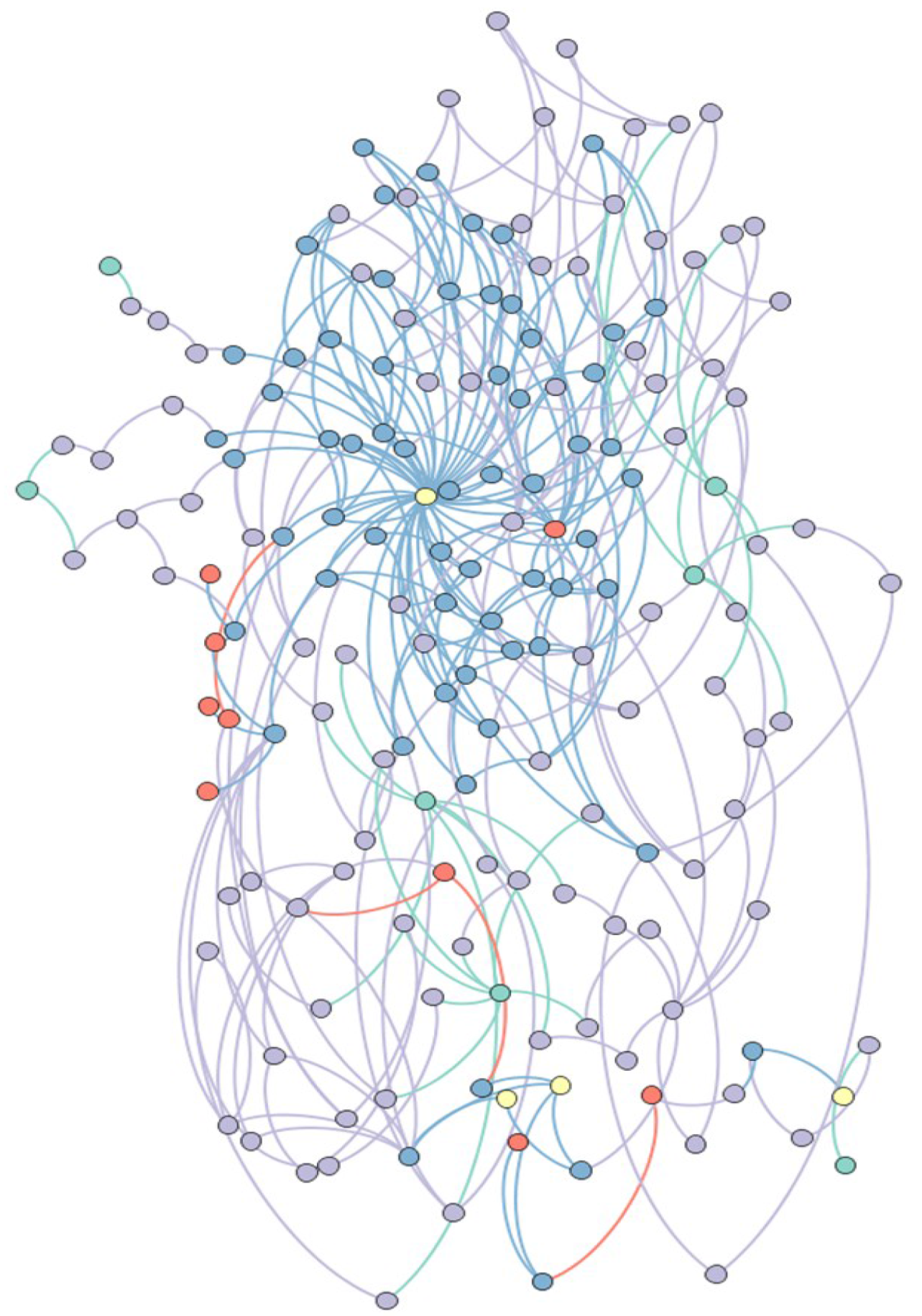
Processes 03 00514 g001
Figure 2. Abstract representation of the bioconversion network used in this study. Yellow nodes correspond to biofuel products, orange nodes correspond to byproducts/intermediates, teal nodes correspond to biomass feedstocks, purple nodes correspond to initial/pretreatment technologies, and blue nodes correspond to final upgrading technologies.
Processes 03 00514 g002
Both indirect and direct process water consumption was retrieved from technoeconomic analyses and design reports (for example, [34,35,36]). Most direct water consumption (e.g., water used for reactions) data were retrieved from analyzing mass flow streams. When direct water consumption was not explicitly provided, the amount of makeup water needed in the process models was used. Indirect water consumption via cooling and heating was taken into account. All input data, including the water consumption rates for each technology, the unit energy consumption rates for each technology, reference capital costs for each technology, reference operating costs for each technology, and yield coefficints for the different technologies and their feeds and products are available as an Excel file in the Supporting Information.
Direct water consumption stemming from biomass cultivation was retrieved from a variety of sources [46]. For example, the cultivation water footprints for many biomass feedstocks were compiled by Mekonnen and Hoekstra (2011) [47], and May et al. [48] analyzed water requirements for softwood plantations. These studies and the present one assume that each biomass crop is grown in arable land with typical amounts of rainfall. Furthermore, this study only investigates fresh water consumption that are in addition to typical amounts of rainfall. Overall, water footprints tended to be higher for highly irrigated crops, such as corn, soybeans, and sugarcane. In contrast, water footprints tended to be very low or negligible for energy crops and woody biomass. Similar water consumption analyses can also be performed for general energy product and process networks. The water consumption of each type of biomass during its cultivation is included in Table 1.
Table 1. Water consumption rates for cultivation of the biomass feedstocks available in this work.
Biomass FeedstockWater Consumption Rate for Cultivation (L/kg Biomass)
Soybean2145
Corn1222
Sugarcane210
Corn Stover1222
Hardwood0.357
Softwood0.268
Switchgrass0
Simulated demands of 10.89 ML/year for ethanol, 11.53 ML/year for gasoline, and 10.32 ML/year for diesel are chosen for each bioconversion case study. These demand levels were chosen to represent a pilot-scale processing pathway with approximately half the capacity relative to a recently built, full scale biofuels plant with total capacity of 76 ML/year [39]. The capital cost of this 76 ML/year plant is also given, providing a basis for a capital cost budget for this work of $250 M. The minimum availability of each biomass type was set to zero, and the maximum availability of each biomass type was set to a large number (100,000 kg/h each) to ensure the solutions would not be constrained by biomass availability. Thus, any amount of biomass between 0 kg/h and 100,000 kg/h could be utilized in the processing pathways. Such an approach was taken to ensure that the chosen pathways of each solution are inherently the most optimal ones. In order to calculate the fixed and variable transportation costs, an average distance of 33.3 miles (approximately 54 km) was chosen as this is the average distance traveled to the center of a circle with a radius of 50 miles, a distance identified to be a maximum viable transportation distance for biofuels [49]. The fixed transportation cost of each biomass type was assumed to be $0.0000048/kg, and the variable transportation cost of each biomass type was assumed to be $0.0000024/kg. Since this study is primarily concerned with investigating the water-energy nexus of bioconversion technologies, only biofuels technologies were included in the case studies. The energy content of each biofuel was taken as its HHV. No bioproducts (e.g., succinic acid, levulinic acid, biopolymers, etc.) technologies were included in the model, as there is no straightforward way to analyze the economic and water footprint impacts of their production from a water-energy nexus perspective. This is done not to imply that production of bioproducts is not promising—Indeed, several studies cite bioproducts as key to enhancing the economic viability of biofuels processes [50,51,52]. However, this possibility is not a focus of this work.
An interest rate r of 10% and a processing pathway lifetime n of 20 years is assumed. The fixed cost factor fcfj is taken as 5% of the capital cost of technology j [40]. Technology selection, sizing, feedstock selection and quantities purchased, levels of the three fuels produced, capital costs, operating costs, and the water footprint are all decision variables. The HHV for each fuel was used to determine the energy efficiency of water for each processing pathway. The case study has a system boundary of “cradle to grave”, and it is assumed that all biomass that is purchased is processed, and all biofuels produced are sold and consumed. Water consumption is tallied from biomass cultivation to biomass processing and fuel production. Current market prices for feedstocks and fuels are used [53,54], and these prices are compiled in Table 2.
Table 2. Market prices of all raw materials (biomass feedstocks) and products (biofuels) available in this work.
Biomass Feedstock/BiofuelMarket Price ($/kg)
Soybean0.1085
Corn0.0317
Sugarcane0.0925
Corn Stover0.0881
Hardwood0.0728
Softwood0.0728
Switchgrass0.0878
Ethanol0.61
Gasoline0.83
Diesel and Biodiesel0.92
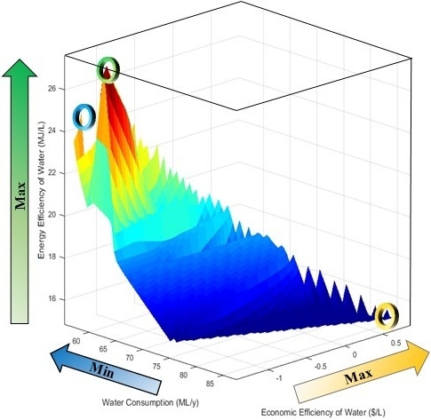
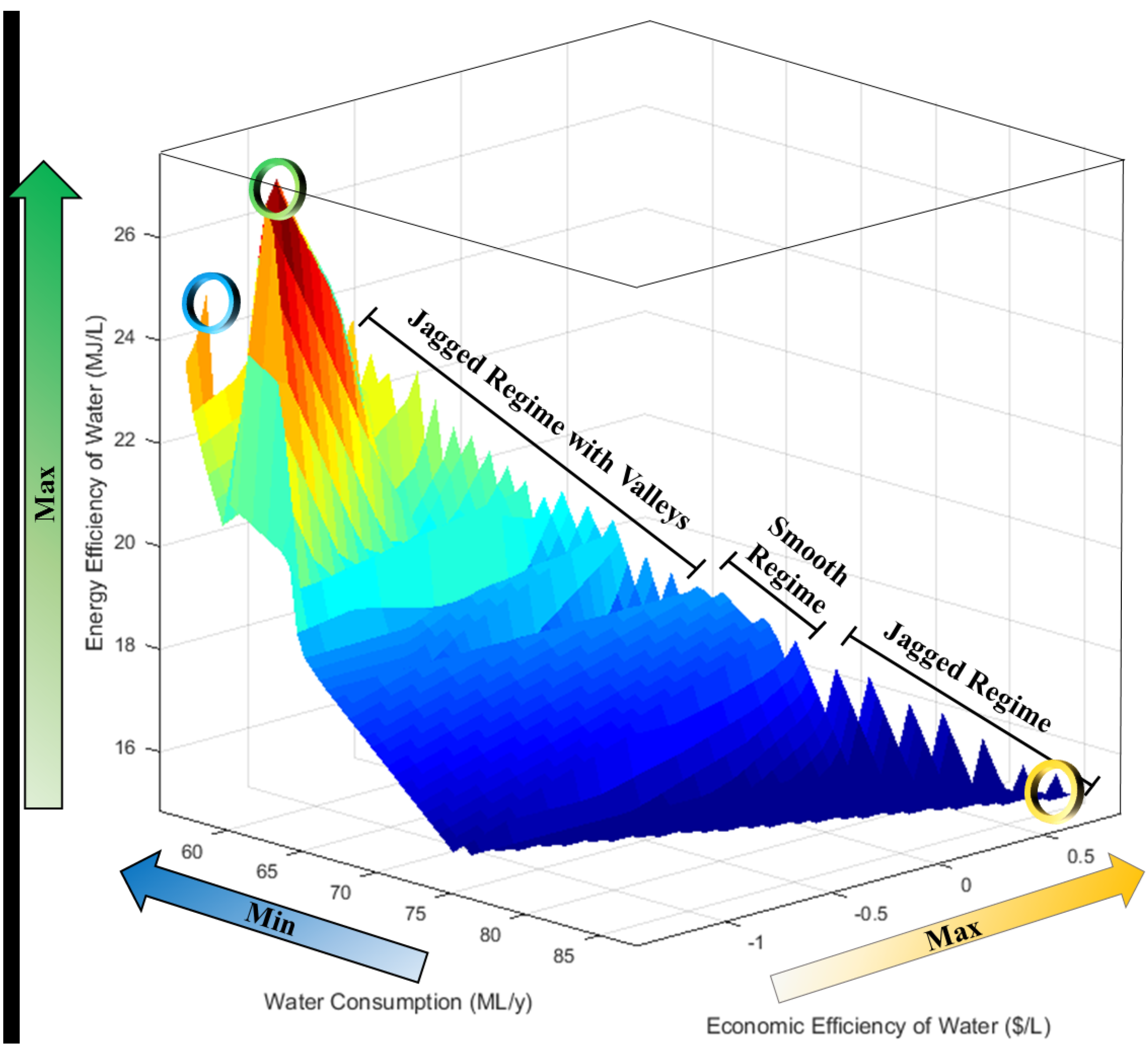
A Pareto-optimal surface displaying the results is shown in Figure 3. Clear trends and tradeoffs between the objective functions are present. In general, as the economic efficiency of water increases, the total water consumption increases and the energy efficiency of water decreases. There are also three distinct regimes following energy efficiency of water changes relative to changes in water consumption rates along the Pareto-optimal surface: A jagged regime, a smooth regime, and a jagged regime with valleys, as shown on Figure 3. A more jagged regime could suggest that the energy efficiency of water is more sensitive to changes in water consumption rates in this regime than a smooth regime. A jagged regime with valleys might imply that changes in the energy efficiency of water are more sensitive to changes in the water consumption rate than in a smooth regime, but not as sensitive as in a jagged regime. Interestingly, the maximum energy efficiency of water and the minimum water consumption points are near each other on the Pareto-optimal surface. This implies that there are synergies between maximizing the water efficiency of energy and minimizing water consumption, a relationship that could have important policy implications. For example, since the energy efficiency of water solution has a better economic efficiency of water than the minimum water consumption solution, this solution might be chosen as something of a “good compromise” solution. Overall, the Pareto-optimal surface provides the decision maker with a thorough overview of the economic, energy, and environmental impacts of their decisions. Furthermore, more informed decisions can be made in the biofuels water-energy nexus depending on which regime the decision maker plans to operate within.
Figure 3. Pareto-optimal surface with key features and extreme points highlighted. The minimum water consumption solution is denoted with a blue circle (far left), the maximum energy efficiency of water solution is denoted with a green circle (middle), and the maximum economic efficiency of water solution is denoted with a yellow circle (right).
Processes 03 00514 g003
Three extreme points exist on the three corners of the Pareto-optimal surface: One denotes the minimum water footprint solution, another denotes the maximum economic efficiency of water solution, and the third point denotes the maximum energy efficiency of water solution. These three solutions are highlighted in Figure 3 and discussed in the following subsections.

3.2. Minimum Water Footprint Solution

The optimal processing pathway with the minimum water footprint is shown in Figure 4 and has a water footprint of 55.1 ML/year. Switchgrass is the only feedstock selected for processing, as it was assumed that no extra water outside of natural rainfall was required for its cultivation. Many of the technologies chosen in the processing pathway were modeled based on technoeconomic analyses that involved water recycling streams for each technology (denoted with a water droplet on the technology in the figure). The demand for gasoline is met exactly, with diesel production exceeding demand because the technology selected produces diesel with a higher yield than gasoline. Ethanol production exceeds minimum demand. This result would seem counterintuitive if the processing pathway for ethanol was independent of gasoline and diesel production. However, upon closer inspection of the processing pathway, this is not the case; the production pathways of all fuels are integrated. This result of surplus ethanol production could be explained by the following observations. In addition to the pyrolysis of switchgrass (after handling and chopping) to produce bio-oil that is subsequently upgraded to gasoline and diesel, residues from distillation and pervaporation processes used to produce ethanol are also pyrolyzed into a bio-oil and subsequently upgraded. Thus, the processing pathway leverages those technologies with high levels of water recycling in the ethanol production pathways to minimize the water footprints of integrated gasoline and diesel production with ethanol production relative to their independent production. As a side effect, a surplus of ethanol is produced relative to demand. Furthermore, this processing pathway also results in the second highest energy efficiency of water at 24.62 MJ/L. This pathway clearly demonstrates the advantages of process integration for minimizing the water footprint. Unfortunately, this processing pathway also reflects the cost of water recycling and process integration in the lowest economic efficiency of water (−$1.31/L) of any of the optimal processing pathways.
Figure 4. Optimal processing pathway, water footprint, economic efficiency of water, overall capital cost, and energy efficiency of water of the minimum water footprint solution. A water drop over a technology in the pathway denotes process water recycling is incorporated in the input process data.
Processes 03 00514 g004

3.3. Maximum Economic Efficiency of Water Solution

The processing pathway with the highest economic efficiency of water is shown in Figure 5. It has an energy efficiency of water of 15.32 MJ/L, an economic efficiency of water of $0.76/L, a water footprint of 87.6 ML/year, and a capital cost of $250 M. Both switchgrass and softwood are used in this pathway. The overall processing pathway is similar to the pathway for the minimum water footprint solution in that ethanol is produced by pretreatment, saccharification and fermentation of hydrolyzates, and distillation of the resulting broth. Gasoline and diesel are again produced by hydrotreating and hydrocracking of pyrolysis products. However, pervaporation technologies are absent in favor of larger, more cost-effective distillation technologies. Hot water pretreatment is also preferred over dilute acid pretreatment due to lower operating costs, despite larger energy costs and higher rates of water use.
Figure 5. Optimal processing pathway, water footprint, economic efficiency of water, overall capital cost, and energy efficiency of water of the maximum economic efficiency of water solution.
Processes 03 00514 g005
Less ethanol is produced in this processing pathway compared to the minimum water footprint solution, implying that producing ethanol is not a profitable venture, even with a myriad of conversion technologies to choose from. Gasoline demand is met exactly, and diesel demand is exceeded as hydrocracking has a higher yield for diesel than gasoline. Interestingly, technologies that employ water recycling are employed extensively in this processing pathway. This selection might appear to work against increasing the economic efficiency of water of the process, as water recycling is expensive. This might be true when maximizing solely the NPV. However, the goal of this solution point is to maximize the economic efficiency of water, or the amount of value the processing pathway can produce from each liter of water consumed. Thus, there is a tradeoff between minimizing the water footprint and maximizing the NPV of the processing pathway. Encouragingly, the economic efficiency of water for this processing pathway is positive, indicating an overall profitable process. Thus, the results show that profits can still be made by producing biofuels while simultaneously considering sustainability impacts such as the water footprint.

3.4. Maximimum Energy Efficiency of Water Solution

Finally, the processing pathway with the maximum energy efficiency of water is shown in Figure 6. As in the minimum water footprint solution, only switchgrass is processed, minimizing the amount of cultivation water used in the processing pathway. Indeed, the same technologies are employed as in the minimum water footprint solution with the difference between the two solutions in the capacities of the selected technologies. The amount of ethanol produced is the largest of either of the previous solutions at 31.4 ML/year. Instead of producing the more energy dense fuels of gasoline and diesel to increase the energy efficiency of water, ethanol production is favored. This phenomenon is likely due to high levels of water recycling in the technologies within the ethanol production pathway. Traditionally, ethanol has been essentially the only biofuel produced in the United States. As a result, various technoeconomic analyses of ethanol production processes have been performed that take into account details such as water recycling and process optimization. Detailed technology development and process optimization for more advanced bioconversion technologies has not been performed, so detailed data concerning recycling of water in these advanced technologies do not yet exist.
Figure 6. Optimal processing pathway, water footprint, economic efficiency of water, overall capital cost, and energy efficiency of water of the maximum energy efficiency of water solution.
Processes 03 00514 g006
An energy efficiency of water of 27.98 MJ/L is the largest energy efficiency of water across all processing pathways, as expected. An economic efficiency of water of −$1.19/L is achieved, a value intermediate between that of the minimum water footprint solution and that of the maximum economic efficiency of water solution. Furthermore, its water footprint of 59.3 ML/year is intermediate between that of the previous two solutions; however, this value is far closer to that of the minimum water footprint solution than that of the maximum economic efficiency of water solution. Thus, this solution could be seen in several ways as a good compromise solution between the two extremes of the minimum water footprint solution and the maximum economic efficiency of water solution. While this solution has the highest energy efficiency of water and intermediate values of the water footprint and economic efficiency of water, its economic efficiency of water is still negative, implying a non-profitable and, ultimately, unrealistic solution. A comparison in computation time between finding this solution by directly solving the model with BARON 14.4 and the proposed pathway with CPLEX 12.6 is shown in the Appendix.
Results presented in this work compare favorably to previous literature on estimated water footprints of biofuels production processes. The energy efficiencies of water in this work ranged from 15.32 MJ/L to 27.98 MJ/L. Wu et al. assessed the water footprints of ethanol production from switchgrass and found that between 1.9 and 9.8 liters of water were required to produce one liter of ethanol [55]. These results correspond to energy efficiencies of water ranging from 0.62 MJ/L to 3.18 MJ/L. Since the results presented in this work are optimal processing solutions, they are larger than the non-optimal results reported in the literature by up to two orders of magnitude. We note that on a liter of water consumed per liter of fuel produced basis (not adjusting for energy content of the fuel), our results range from 1.04 to 2.02, which are similar to the lower range of the results of Wu et al. They also found that using corn to produce ethanol with traditional methods requires 10–17 liters of water per liter of ethanol produced, a far less efficient method than using switchgrass. Other sources state more optimistic results of approximately three liters of water per liter of ethanol, a water footprint that is still higher than the values found in our work [56]. Our results reflect these estimates: Only switchgrass is used to produce ethanol when considering the processing pathway’s water footprint, and corn is not used in any of the optimal solutions. This result has been found elsewhere in the literature; Kantas et al. found that converting switchgrass to ethanol was the most profitable and preferred option when considering water consumption of the process [27].
All results for each extreme point are compiled in Table 3 for convenience and clarity. Each pathway reaches the maximum allowable capital cost of $250 M, and all have similar amounts of produced energy in the form of biofuels per year. The largest differences between the solutions are in their respective economic efficiencies of water, highlighting how critical it still is to further optimize and develop bioconversion technologies to be simultaneously economically competitive and sustainable.
Table 3. Compilation of results for the three optimization scenarios.
MetricMinimum Water FootprintMaximum Economic Efficiency of WaterMaximum Energy Efficiency of Water
Energy Produced (in Biofuel Form) (MJ/year)1.34 × 1091.56 × 1091.66 × 109
Water Footprint (ML/year)55.187.659.3
Energy Efficiency of Water (MJ/L)24.6215.3227.98
Capital Cost ($M)250250250
Economic Efficiency of Water ($/L)−1.310.76−1.19
Overall, modeling and optimization of biofuels product and process networks was shown to provide meaningful insight to the water-energy nexus of biofuels. The results herein could also have significant policy implications. For example, it is immediately apparent that feedstocks that require minimal water for cultivation should be utilized for energy production compared to highly irrigated crops, such as corn or soybeans. Thus, decision makers should consider using feedstocks such as switchgrass or woody biomass to produce biofuels. Results obtained from the case study with maximizing the energy efficiency of water as the objective resulted in a relatively low water footprint paired with the best use of water resources in the context of energy production. Furthermore, while still economically unviable, it is less unprofitable than minimizing the water footprint directly. Thus, policymakers and other decision makers might look to use the energy efficiency of water as a metric to create policies for the water-energy nexus of both biofuels systems and other energy systems. Consideration must be given, however, to the economics of the system. In this case study, if the solution with the maximum energy efficiency of water is chosen by policymakers or other decision makers, then some sort of economic subsidy would also be required for successful implementation.

4. Conclusions

A general multiobjective modeling and solution strategy for the optimization of the water-energy nexus of energy product and process networks was established. Through a bioconversion case study, this model and solution strategy was used to optimize the water-energy nexus of a biofuels product and process network. “Liters of water consumed” was chosen as the functional unit for the “cradle to grave” life cycle optimizations. Three optimal processing pathways were identified from the extreme points of the Pareto-optimal surface. One pathway reflected a bioconversion processing pathway with a minimized water footprint. Another provided a pathway with a maximized NPV per unit amount of water consumed (the economic efficiency of water), and a third pathway represented a maximized energy efficiency of water. The novel processing pathways that result from each extreme point show improvement in the energy efficiency of water compared to literature sources. Switchgrass and softwood feedstocks—feedstocks that require very little additional water input during cultivation—were used in each processing pathway and were used exclusively in the minimum water footprint and maximum energy efficiency of water solutions. Thus, if water preservation is seen as an important consideration of production of biofuels, these results could suggest that energy crops or woody biomass might be optimal feedstock candidates.
A novel solution method for optimizing the water-energy nexus of process and product networks in a life cycle optimization context was developed. The parametric algorithm was paired with a branch and refine algorithm using successive piecewise linear approximations to nonconvex terms and NLP subproblems to the original MINLFP problem to ensure feasibility and global convergence. The proposed method was shown to have improved computational performance compared to directly solving the MINLFP problem with off-the-shelf global solvers, performing an order of magnitude faster. As the product and process network grows larger and more sustainability objectives are added, this improved performance could prove valuable.

Supplementary Files

Supplementary File 1

Acknowledgments

We gratefully acknowledge the financial support from the Institute for Sustainability and Energy at Northwestern University (ISEN) and Argonne National Laboratory via a Northwestern-Argonne Early Career Investigator Award for Energy Research.

Author Contributions

D.J.G. collected the data and developed the model; F.Y. conceived the research concept; D.J.G. and F.Y. analyzed the results and wrote the manuscript.

Conflicts of Interest

The authors declare no conflict of interest.

Appendix

A.1. Notation

Sets
ISet of materials/compounds
JSet of technologies
NSet of points in the piecewise linear approximations
Subsets
BSubset of biomass feedstocks
FSubset of biofuel products
Continuous Variables
CCjCapital cost of technology j
FEEnergy available in all final fuel products
NPVAnnualized net present value of the processing pathway
OBJEcEWObjective function for the economic efficiency of water
OBJEEWObjective function for the energy efficiency of water
OBJwaterObjective function for the water footprint
PiAmount of biomass feedstock i purchased
SiAmount of biofuel product i produced and sold
Wj,nWeighted variable to determine where along the piecewise linear approximations in interval n the solution lies for technology j
WFThe water footprint of the processing pathway
XjThe capacity of technology j
Discrete Variables
BDjA decision variable that determines if technology j is included in the final processing pathway
SOS1 Variables
EXj,nSOS1 variable that ensures only one solution is present for technology j along the piecewise linear approximations for technology j over intervals n
Parameters
ccbThe capital cost budget of the processing pathway
ccfCapital cost factor
cchfCapital charge factor
demiThe demand to be satisfied for fuel i
dyijThe destructive yield of compound/material i in technology j
ecCost of electricity
fcfjThe fixed cost factor for technology j
fpiPrice of feedstock i
ftciDistance-fixed transportation cost for feedstock i
mnaiMinimum availability for feedstock i
mxaiMinimum availability for feedstock i
nExpected lifetime of the processing pathway
peciProduct energy content of fuel product i
pyijProductive yield of compound/material i in technology j
qeParametric parameter for the economic efficiency of water objective
qnParametric parameter for the energy efficiency of water objective
rInterest rate
refcjReference capacity of technology j
refccjReference capital cost of technology j
refocjReference operating cost of technology j
sfjCapital cost scaling factor for technology j
spiThe selling price of compound/material i
uj,nParameter used to represent the capacity of technology j at point n of the piecewise linear approximation
uejUnit electricity requirement of technology j
valj,nParameter used, along with the variable Wj,n, to represent the capital cost of technology j at point n of the piecewise linear approximation
vtciVariable transportation cost of feedstock i
wciUnit rate of water consumption for cultivation of feedstock i
wpjUnit rate of water consumption of technology j
εFEε-constraint parameter for the energy efficiency of energy
εNPVε-constraint parameter for the economic efficiency of water

A.2. Computational Performance Results

Computational results for maximizing the energy efficiency of water are shown in Table A.1. The problem is solved with both BARON 14.4.0 and the proposed MILP method with NLP subproblems outlined in the previous section. Both methods provided the same globally optimal solution of 27.98 MJ/L for the energy efficiency of energy. However, the proposed method solves the problem an order of magnitude faster than the original MINLP problem with BARON 14.4.0. This increase in computational performance is observed even with an increase in problem size from the original MINLP problem to the proposed method, reflecting the efficiency of the underlying algorithm. The MILP problem has 4112 constraints and 4291 continuous variables compared to 1512 constraints and 891 continuous variables in the original MINLP problem. As the bioconversion network increases in size or if the network model is incorporated into a multiobjective optimization model, the improved computational performance offered by the proposed method could prove to be indispensable for quick and efficient identification of globally optimal solutions.
Table A.1. Comparative computational results for calculating the maximum energy efficiency of water solution point.
Model PropertyOriginal MINLFP ProblemMILP with NLP Subproblems
Objective Value (MJ/L)27.9827.98
Constraints1,5124112 (MILP); 1512 (NLP subproblems)
Continuous Variables8914291 (MILP); 891 (NLP subproblem)
Discrete Variables200400 (MILP); 0 (NLP subproblem)
SolverBARON 14.4.0CPLEX 12.6.1/CONOPT3
Solution Time (CPUs)56.57.6

References

  1. Bakshi, B.R.; Fiksel, J. The quest for sustainability: Challenges for process systems engineering. AIChE J. 2003, 49, 1350–1358. [Google Scholar] [CrossRef]
  2. Bakshi, B.R. Methods and tools for sustainable process design. Curr. Opin. Chem. Eng. 2014, 6, 69–74. [Google Scholar] [CrossRef]
  3. Watkins, K. Human Development Report 2006-beyond Scarcity: Power, Poverty and the Global Water Crisis; UNDP: New York, NY, USA, 2006. [Google Scholar]
  4. Carlton, J.; Lazo, A.U.S. News: California declares drought emergency. Wall Street Journal 2014, A.3. [Google Scholar]
  5. Bagajewicz, M.; Rodera, H.; Savelski, M. Energy efficient water utilization systems in process plants. Comput. Chem. Eng. 2002, 26, 59–79. [Google Scholar] [CrossRef]
  6. Alnouri, S.; Stijepovic, M.; Linke, P.; El-Halwagi, M. Optimal design of spatially constrained interplant water networks with direct recycling techniques using genetic algorithms. Chem. Eng. Trans. 2014, 39, 457–462. [Google Scholar]
  7. Sueviriyapan, N.; Siemanond, K.; Quaglia, A.; Gani, R.; Suriyapraphadilok, U. The optimization-based design and synthesis of water network for water management in an industrial process: Refinery effluent treatment plant. Chem. Eng. 2014, 39, 133–138. [Google Scholar]
  8. Kenny, J.F.; Barber, N.L.; Hutson, S.S.; Linsey, K.S.; Lovelace, J.K.; Maupin, M.A. Estimated Use of Water in the United States in 2005; US Geological Survey: Reston, VA, USA, 2009.
  9. U.S. Department of Energy. The Water-Energy Nexus: Challenges and Opportunities; U.S. Department of Energy: Washington, DC, USA, 2014.
  10. Hussey, K.; Pittock, J. The energy-water nexus: Managing the links between energy and water for a sustainable future. Ecol. Soc. 2012. [Google Scholar] [CrossRef]
  11. Carter, N.T. Energy’s Water Demand: Trends, Vulnerabilities, and Management; DIANE Publishing: Darby, PA, USA, 2011. [Google Scholar]
  12. Perrone, D.; Murphy, J.; Hornberger, G.M. Gaining perspective on the water-energy nexus at the community scale. Environ. Sci. Technol. 2011, 45, 4228–4234. [Google Scholar] [CrossRef] [PubMed]
  13. USGS. Hydroelectric Power Water Use. Available online: http://water.usgs.gov/edu/wuhy.html (accessed on 7 July 2015).
  14. Herath, I.; Deurer, M.; Horne, D.; Singh, R.; Clothier, B. The water footprint of hydroelectricity: A methodological comparison from a case study in new zealand. J. Clean. Prod. 2011, 19, 1582–1589. [Google Scholar] [CrossRef]
  15. Jiménez-Gutiérrez, A.; Lona-Ramírez, J.; Ponce-Ortega, J.M.; El-Halwagi, M. An minlp model for the simultaneous integration of energy, mass and properties in water networks. Comput. Chem. Eng. 2014, 71, 52–66. [Google Scholar] [CrossRef]
  16. Gao, J.; You, F. Optimal design and operations of supply chain networks for water management in shale gas production: Milfp model and algorithms for the water-energy nexus. AIChE J. 2015, 61, 1184–1208. [Google Scholar] [CrossRef]
  17. Murphy, C.F.; Allen, D.T. Energy-water nexus for mass cultivation of algae. Environ. Sci. Technol. 2011, 45, 5861–5868. [Google Scholar] [CrossRef] [PubMed]
  18. Walker, M.E.; Lv, Z.; Masanet, E. Industrial steam systems and the energy-water nexus. Environ. Sci. Technol. 2013, 47, 13060–13067. [Google Scholar] [CrossRef] [PubMed]
  19. Ahmetovic, E.; Martín, M.; Grossmann, I.E. Optimization of energy and water consumption in corn-based ethanol plants. Ind. Eng. Chem. Res. 2010, 49, 7972–7982. [Google Scholar] [CrossRef]
  20. Baliban, R.C.; Elia, J.A.; Floudas, C.A. Simultaneous process synthesis, heat, power, and water integration of thermochemical hybrid biomass, coal, and natural gas facilities. Comput. Chem. Eng. 2012, 37, 297–327. [Google Scholar] [CrossRef]
  21. Halim, I.; Srinivasan, R. Sequential methodology for integrated optimization of energy and water use during batch process scheduling. Comput. Chem. Eng. 2011, 35, 1575–1597. [Google Scholar] [CrossRef]
  22. Elena, G.-C.; Esther, V. From water to energy: The virtual water content and water footprint of biofuel consumption in spain. Energy Policy 2010, 38, 1345–1352. [Google Scholar] [CrossRef]
  23. Gheewala, S.H.; Berndes, G.; Jewitt, G. The bioenergy and water nexus. Biofuels Bioprod. Biorefining 2011, 5, 353–360. [Google Scholar] [CrossRef]
  24. Cobuloglu, H.I.; Büyüktahtakın, İ.E. Food vs. Biofuel: An optimization approach to the spatio-temporal analysis of land-use competition and environmental impacts. Appl. Energy 2015, 140, 418–434. [Google Scholar] [CrossRef]
  25. Grossmann, I.E.; Martín, M. Energy and water optimization in biofuel plants. Chin. J. Chem. Eng. 2010, 18, 914–922. [Google Scholar] [CrossRef]
  26. Čuček, L.; Martín, M.; Grossmann, I.E.; Kravanja, Z. Energy, water and process technologies integration for the simultaneous production of ethanol and food from the entire corn plant. Comput. Chem. Eng. 2011, 35, 1547–1557. [Google Scholar] [CrossRef]
  27. Kantas, A.B.; Cobuloglu, H.I.; Büyüktahtakιn, İ.E. Multi-source capacitated lot-sizing for economically viable and clean biofuel production. J. Clean. Prod. 2015, 94, 116–129. [Google Scholar] [CrossRef]
  28. You, F.; Wang, B. Life cycle optimization of biomass-to-liquid supply chains with distributed-centralized processing networks. Ind. Eng. Chem. Res. 2011, 50, 10102–10127. [Google Scholar] [CrossRef]
  29. Yue, D.; Kim, M.A.; You, F. Design of sustainable product systems and supply chains with life cycle optimization based on functional unit: General modeling framework, mixed-integer nonlinear programming algorithms and case study on hydrocarbon biofuels. ACS Sustain. Chem. Eng. 2013, 1, 1003–1014. [Google Scholar] [CrossRef]
  30. Yue, D.; Slivinsky, M.; Sumpter, J.; You, F. Sustainable design and operation of cellulosic bioelectricity supply chain networks with life cycle economic, environmental, and social optimization. Ind. Eng. Chem. Res. 2014, 53, 4008–4029. [Google Scholar] [CrossRef]
  31. You, F.; Tao, L.; Graziano, D.J.; Snyder, S.W. Optimal design of sustainable cellulosic biofuel supply chains: Multiobjective optimization coupled with life cycle assessment and input-output analysis. AIChE J. 2012, 58, 1157–1180. [Google Scholar] [CrossRef]
  32. Gong, J.; You, F. Global optimization for sustainable design and synthesis of algae processing network for CO2 mitigation and biofuel production using life cycle optimization. AIChE J. 2014, 60, 3195–3210. [Google Scholar] [CrossRef]
  33. Garcia, D.J.; You, F. Multiobjective optimization of product and process networks: General modeling framework, efficient global optimization algorithm, and case studies on bioconversion. AIChE J. 2015, 61, 530–554. [Google Scholar] [CrossRef]
  34. Zhu, Y.; Biddy, M.J.; Jones, S.B.; Elliott, D.C.; Schmidt, A.J. Techno-economic analysis of liquid fuel production from woody biomass via hydrothermal liquefaction (HTL) and upgrading. Appl. Energy 2014, 129, 384–394. [Google Scholar] [CrossRef]
  35. Obernberger, I.; Thek, G. Techno-Economic Evaluation of Selected Decentralised Chp Applications Based on Biomass Combustion, Iea Partner-Final Report; IEA: Graz, Austria, 2004. [Google Scholar]
  36. Zhu, Y.; Jones, S.B. Techno-Economic Analysis for the Thermochemical Conversion of Lignocellulosic Biomass to Ethanol via Acetic Acid Synthesis; PNNL: Richland, WA, USA, 2009. [Google Scholar]
  37. ISO. Environmental Management: Life Cycle Assessment: Principles and Framework; ISO: Geneva, Switzerland, 1997; Volume 14040. [Google Scholar]
  38. Cai, X.; Rosegrant, M.W.; Ringler, C. Physical and economic efficiency of water use in the river basin: Implications for efficient water management. Water Resour. Res. 2003, 39. [Google Scholar] [CrossRef]
  39. POET-DSM Advanced Biofuels, L. First commercial-scale cellulosic ethanol plant in the U.S. Opens for business. Available online: http://poet-dsm.com/pr/first-commercial-scale-cellulosic-plant (accessed on 7 July 2015).
  40. Seider, W.D.; Seader, J.D.; Lewin, D.R.; Widagdo, S. Product and Process Design Principles, 3rd ed.; John Wiley & Sons, Inc.: Hoboken, NJ, USA, 2009. [Google Scholar]
  41. You, F.; Grossmann, I.E. Stochastic inventory management for tactical process planning under uncertainties: Minlp models and algorithms. AIChE J. 2011, 57, 1250–1277. [Google Scholar] [CrossRef]
  42. Zhong, Z.; You, F. Globally convergent exact and inexact parametric algorithms for solving large-scale mixed-integer fractional programs and applications in process systems engineering. Comput. Chem. Eng. 2014, 61, 90–101. [Google Scholar] [CrossRef]
  43. Hasan, M.M.F.; Karimi, I.A. Piecewise linear relaxation of bilinear programs using bivariate partitioning. AIChE J. 2010, 56, 1880–1893. [Google Scholar] [CrossRef]
  44. Brooke, A.; Kendrick, D.; Meeraus, A.; Rosenthal, R.E. Gams: A User’s Guide: Course Technology; GAMS Development Corporation: Washington, DC, USA, 1988. [Google Scholar]
  45. Tawarmalani, M.; Sahinidis, N. A polyhedral branch-and-cut approach to global optimization. Math. Program. 2005, 103, 225–249. [Google Scholar] [CrossRef]
  46. Wu, M.; Mintz, M.; Wang, M.; Arora, S. Water consumption in the production of ethanol and petroleum gasoline. Environ. Manag. 2009, 44, 981–997. [Google Scholar] [CrossRef] [PubMed]
  47. Mekonnen, M.M.; Hoekstra, A.Y. The green, blue and grey water footprint of crops and derived crop products. Hydrol. Earth Syst. Sci. 2011, 15, 1577–1600. [Google Scholar] [CrossRef]
  48. May, B.; England, J.R.; Raison, R.J.; Paul, K.I. Cradle-to-gate inventory of wood production from australian softwood plantations and native hardwood forests: Embodied energy, water use and other inputs. For. Ecol. Manag. 2012, 264, 37–50. [Google Scholar] [CrossRef]
  49. Khosla, V. Where Will Biofuels and Biomass Feedstocks Come from? Khosla Ventures: Menlo Park, CA, USA, 2008; p. 31. [Google Scholar]
  50. Bozell, J.J. Connecting biomass and petroleum processing with a chemical bridge. Science 2010, 329, 522–523. [Google Scholar] [CrossRef] [PubMed]
  51. Dunn, J.B.; Adom, F.; Sather, N.; Han, J.; Snyder, S.W. Life-Cycle Analysis of Bioproducts and their Conventional Counterparts in Greet; Argonne National Laboratory: Argonne, IL, USA, 2014.
  52. Gong, J.; You, F. Value-added chemicals from microalgae: Greener, more economical, or both? ACS Sustain. Chem. Eng. 2015, 3, 82–96. [Google Scholar] [CrossRef]
  53. Mundi, I. Select commodity price indices. Available online: http://www.indexmundi.com/commodities/ (accessed on 7 July 2015).
  54. ProgressiveFarmer. Daily Ethanol Rack Prices. Available online: http://www.dtnprogressivefarmer.com/dtnagcommon/link.do;jsessionid=5EB7BC182389FFB24ED238D3F34346D8.agfreejvm2?symbolicName=RENEWABLE_FUELS_PAGE_FREE (accessed on 7 July 2015).
  55. Wu, M.; Wang, M.; Liu, J.; Huo, H. Life-Cycle Assessment of Corn-Based Butanol as a Potential Transportation Fuel; ANL: Argonne, IL, USA, 2007.
  56. University of Illinois. Water Use for Ethanol Production; University of Illinois: Urbana-Champaign, Illinois, IL, USA, 2009. [Google Scholar]

