Analyzing the Mixing Dynamics of an Industrial Batch Bin Blender via Discrete Element Modeling Method

Abstract

A discrete element model (DEM) has been developed for an industrial batch bin blender in which three different types of materials are mixed. The mixing dynamics have been evaluated from a model-based study with respect to the blend critical quality attributes (CQAs) which are relative standard deviation (RSD) and segregation intensity. In the actual industrial setup, a sensor mounted on the blender lid is used to determine the blend composition in this region. A model-based analysis has been used to understand the mixing efficiency in the other zones inside the blender and to determine if the data obtained near the blender-lid region are able to provide a good representation of the overall blend quality. Sub-optimal mixing zones have been identified and other potential sampling locations have been investigated in order to obtain a good approximation of the blend variability. The model has been used to study how the mixing efficiency can be improved by varying the key processing parameters, i.e., blender RPM/speed, fill level/volume and loading order. Both segregation intensity and RSD reduce at a lower fill level and higher blender RPM and are a function of the mixing time. This work demonstrates the use of a model-based approach to improve process knowledge regarding a pharmaceutical mixing process. The model can be used to acquire qualitative information about the influence of different critical process parameters and equipment geometry on the mixing dynamics.

1. Introduction

Powder mixing is a widely implemented unit operation in several particulate processing industries (e.g., food, pharmaceutical, chemical, etc.) for combining two or more raw materials in the required proportions into a final blend (mixture). Uniformity in the composition of the final blend is a key requirement and has a considerable influence on the quality of the final product. Since mixing dictates the uniformity in the composition of the blend, which is then sent for further downstream processing, the performance of this particular operation is critical to the operational efficiency of these industries [1]. Various industrial blenders with different mixing mechanisms are available and can be chosen based on the processing requirements. For example, tumbling blenders are often implemented for mixing granular materials, and a bin blender is the most commonly-used variation of the tumbling blender in the pharmaceutical industries, due to a high level of safety and convenience [2]. However, due to the presence of multiple zones, which demonstrate different mixing behavior in a tumbling blender, understanding the process dynamics in detail would be beneficial for optimal process design. These zones have variable blend uniformity (e.g., presence of super-potent and sub-potent zones). Moreover, as pharmaceutical industries often have to deal with fine powders, which have poor flowability or tend to segregate, mixing them efficiently may become quite challenging [3]. In general, powder flow processes are erratic and have an inherent variability associated with them, due to which various flow analyzing methods (experimental or modeling) are required to obtain a good prediction of their behavior. Mathematical model frameworks developed from physical principles and calibrated with experimental data would aid in providing better process understanding and could prove to be a more resource- and time-saving alternative when compared to other experimental methods for the process design and optimization analysis. The various model-based tools that can be used for process development are predictive models, flexibility and feasibility analysis, steady state and dynamic optimization, sensitivity analysis and controller design [4].

Tolerance in the variability of the blend composition depends on the application, which in the case of pharmaceutical industries is narrow as they need to comply with the stringent product quality norms specified by the regulatory authorities (e.g., United States Food and Drug Administration (USFDA)). A more robust and science-based process design methodology is being implemented in the pharmaceutical industries, to ensure the retention of the detailed process knowledge and re-assess the various product quality risks and uncertainties associated with these. Good product quality can be realized by designing robust manufacturing processes by incorporation thorough process knowledge. Managing and retaining an explicit process knowledge throughout the product life-cycle is an important aspect, as stated in the guidance developed by the International Conference on Harmonisation of Technical Requirements for Registration of Pharmaceuticals for Human Use (ICH): ICH-Q10 [5].

A detailed mathematical model that is validated, well-tuned and calibrated can be used as an efficient tool for pharmaceutical manufacturing process development studies [6], which will help to outline the design space. The design space is defined as “the multidimensional combination and interaction of input variables (e.g., material attributes) and process parameters that have been demonstrated to provide assurance of quality” (ICH: Q8 (R2)). A batch mixing operation involves a large parametric space, which consists of processing parameters (i.e., blender RPM, fill level, loading order), equipment design, material properties, etc. [2,7]. A process consists of several input parameters, but only some are highly sensitive and critical towards the optimal operational efficiency of the process. Therefore, identifying the critical process parameters (CPPs) and understanding their effect on the process efficiency is an important step in establishing the design space and evaluating how effectively the process can withstand any parametric variability without a negative impact on the product quality. The manufacturing steps implemented by the pharmaceutical industries must meet the good manufacturing practices (GMP) guidelines to achieve high process efficiency and good product quality as outlined by the USFDA. This will also allow the product quality to be built consistently in each and every step of the manufacturing process as per the QbD (quality by design) and PAT (process analytical technology) guidelines.

PAT has been defined as “a system for designing, analyzing, and controlling manufacturing through timely measurements of critical quality and performance attributes of raw and in-process materials and processes with the goal of ensuring final product quality” (ICH: Q8 (R2) [6]). It recommends the implementation of measurement and control tools for the CPPs and material properties in the process so that the desired product quality can be obtained. The process variables and parameters must be maintained within the acceptable limits, and any deviation may lead to the production of inferior quality product and also result in process failure, which may have a hazardous impact on the environment, health, safety, etc. A mathematical model can also aid in the design and evaluation of an efficient control loop system based on the process understanding. In short, a process model can be used for virtual experimentation and can be a prerequisite for the design, analysis, control and optimization studies of a process.

Another important step in the design stage of a manufacturing process is process risk analysis. Risk has been defined as “the combination of the probability of occurrence of harm and the severity of that harm” (ICH: Q9). It is necessary to formulate an effective risk management process that is comprised of analyzing and assessing the risks associated with a process (i.e., environmental, health, safety, etc.). A robust risk management process includes several steps, which are risk assessment (risk identification, risk analysis, risk evaluation), risk control (risk reduction, risk acceptance), followed by reviewing the outputs of the risk management process [8]. A good understanding of the potential risks will lead to a reduction in prediction uncertainties and increase the sustainability of the process. Model-based tools can be excellent aids for evaluating the process risks as they can be used to gain process knowledge, identify the CPPs and understand the inter-dependence of the CPPs. These models can then be applied to optimization studies and sensitivity analysis and designing efficient control systems.

1.1. Problem Statement

In the bin blender studied here, three different types of raw materials with different particle sizes and densities have been mixed, and it is hypothesized that multiple zones with different mixing dynamics may be present. At present, the blend composition in the industrial setup is obtained with the aid of a sensor, which is mounted on the lid of the blender. This sensor is able to detect the composition in the near-lid region only and performs a reading every time the bin is inverted. However, it is unknown if the data obtained at the lid are representative of the overall variability of the entire blend due to the scope of the sensor being limited to a tiny volume of the blender. Thief sampling interrupts the process and is invasive. It has also been shown to be unreliable [9]. Since the scale of the blender is large (800 liters), obtaining data about the bulk would also be challenging. Hence, a DEM study has been conducted to test whether composition measurements made at the near-lid zone are able to represent the overall variability in the blend composition [10].

1.2. Objectives

In this work, a discrete element model for an industrial batch bin blender has been presented, and the mixing dynamics have been studied in terms of the blend composition at different locations inside the blender. The blend composition information has been further translated into RSD and intensity of segregation and used to investigate the objectives specified below:

• Determine if the composition measured near the blender lid can be utilized to estimate the variability in the bulk mixture
• Identify the areas of segregation (i.e., super-potent and sub-potent regions)
• Identify the key processing parameters and evaluate the mixing dynamics by varying them
• Demonstrate how a model-based method could be used to recommend more optimal operational parameters and improve the operational efficiency of the mixing operation

2. Background

DEM is often used to simulate powder flow as it treats the particles as discrete entities and is able to track the flow-field of individual particles. The mathematical formulation of DEM is derived from first-principles. DEM calculates the total force acting on the particles due to particle-particle contacts and particle-boundary contacts (contact forces) and other body forces, for example the force of gravity. It then computes the acceleration or velocity using Newton’s second law and updates the particle position based on the velocity information. Two types of forces, normal pressure force and tangential frictional force, act on the particles due to contact. The contact forces are calculated from the various contact models that are available (i.e., Hertzian normal contact force model, Cundall and Stack normal force model, J-K-Rnormal and adhesive force model for cohesive particles, Mindlin–Deresiewicz/Coulomb friction tangential force model, etc.) [11]. In this work, the Hertzian normal contact force model and Mindlin–Deresiewicz tangential force model have been used, as the present model simulates free-flowing non-cohesive powders. The Hertzian normal contact force model assumes a non-linear spring-dashpot model and is applicable within elastic limits for spherical and smooth particles with continuous surface and undergoing non-conforming contact. As detailed by Kruggel-Emden et al. [12], particle-particle contact is detected between two spherical particles when the distance between their centers is less than the sum of their radii; and a particle-boundary contact is detected when the distance between the particle center and the boundary is less than the particle radius. However, a very small overlap (or deformation) may be allowed. As shown in Equation (1), the total force ($\overrightarrow{F}$) acting on the particles is the summation of the normal contact force ($\overrightarrow{F_C^N}$), tangential/frictional contact force ($\overrightarrow{F_C^T}$) and body force ($\overrightarrow{F_B}$). In a bin blender model, the only body force acting may be due to gravity.

$$\overrightarrow{F}=\overrightarrow{F_C^N}+\overrightarrow{F_C^T}+\overrightarrow{F_B}$$

(1)

The acceleration of the particles is calculated from Newton’s law $m\overrightarrow{a}=\overrightarrow{F}$, where m is the particle mass and $\overrightarrow{a}$ is the acceleration vector. The position of the particles is updated from Euler’s equations of rotational motion as shown in Equation (3) [13]. Here, x, y and z are the spatial coordinates of the particle position; I is the moment of inertia; $\overrightarrow{\mathrm{\Omega }}$ is the angular velocity vector; and $\overrightarrow{\tau }$ is the torque.

$$\begin{array}{c}\hfill I_{xx}{\overrightarrow{\omega }}_x+(I_{zz}-I_{yy}){\overrightarrow{\omega }}_z{\overrightarrow{\omega }}_y={\overrightarrow{\tau }}_x\\ \hfill I_{yy}{\overrightarrow{\omega }}_y+(I_{xx}-I_{zz}){\overrightarrow{\omega }}_x{\overrightarrow{\omega }}_z={\overrightarrow{\tau }}_y\\ \hfill I_{zz}{\overrightarrow{\omega }}_z+(I_{yy}-I_{xx}){\overrightarrow{\omega }}_y{\overrightarrow{\omega }}_x={\overrightarrow{\tau }}_z\end{array}$$

(2)

The normal or tangential contact forces are calculated as $\overrightarrow{F_C}=-k{\delta }^{3/2}-\gamma \dot{\delta }{\delta }^{1/4}$. Here, $\overrightarrow{F_C}$ is the normal or tangential contact force; $\delta$ is the normal or tangential overlap; k is the stiffness coefficient factor; $\dot{\delta }$ is the rate of normal or tangential deformation; and $\gamma$ is the damping coefficient. The detailed expressions of these parameters have been given by Dubey et al. [13]. The stiffness coefficient controls the particle stiffness and is a function of the particle size and other material properties (i.e., Poisson’s ratio and Young’s modulus). The stiffness of a body can be defined as its ability to resist deformation when a force is applied on it. Fine tuning of the values of Poisson’s ratio and Young’s modulus is important because it decides the stiffness of the particles, which on the other hand controls the particle deformation or overlap upon contact. It is suggested that the particle overlap be controlled so that the model stays within the elastic limit [14].

DEM has been used to simulate various granular processes. DEM is considered as an explicit particle level model because it treats the particles as discrete entities and is able to capture the effect of equipment geometry, material properties and different particle-particle and particle-geometry interactions on the basis of the forces acting due to different contacts. It is an excellent tool to obtain fundamental particle level information, which is not possible based on other modeling techniques which have been used to model powder systems (i.e., population balance models (PBM) [15], continuum models [16], Markov chain models [17], etc.). DEM can be effectively used for performing qualitative process analysis, process design and optimization, equipment design studies (e.g., determining if any dead zones are present based on the flow pattern), scale-up studies, troubleshooting practical processing issues, etc.

DEM has been used widely to study different kinds of batch and continuous blenders with different mixing mechanisms for both free-flowing and cohesive particles. For example, previous works present extensive studies on the mixing dynamics of the V-blender [18], conical blender [19], slant conical blender [20], rotating drums [21] and other continuous processing blenders [15,22]. Chaudhuri et al. studied the mixing of cohesive particles in a tumbling blender [7]. Bin blenders, in particular, have been studied explicitly by other researchers using DEM. Segregation studies were conducted by Sudah et al. [23] in bin blenders for different loading conditions and fill levels using mono-disperse spheres. Particle movement by convection in the radial direction was shown to be dominant over dispersion in the axial direction inside a bin blender with the help of a DEM model [2]. Using a GPU-based DEM model, it was found that installing the blender at an inclined angle improved the mixing performance of a bin blender [24]. Ren et al. [25] also studied the effect of different numbers and lengths of baffles on the mixing dynamics inside a Gallay tote bin blender. Lemieux et al. compared the flow behaviors of a bin blender and a V-blender for different loading profiles [26]. Detailed analysis of the mixing mechanism and the effect of processing conditions on the mixing dynamics have been investigated in these studies. The present work outlines the steps involved in the implementation of the discrete element methodology to create a model of an industrial-scale tumbling bin blender. The model has been used to investigate the effectiveness of sampling locations in determining the blend homogeneity inside the blender and also to study how the mixing performance inside the blender could be improved.

3. Mathematical Model Development

This section gives an overview of the model development steps that have been followed. The model setup is discussed first, followed by the methods used to calibrate DEM input parameters (particle size, number of particles, shear modulus, Poisson’s ratio, particle-particle and particle-wall coefficients of static and rolling friction, coefficient of restitution), and lastly, the final simulation parameters have been presented. It should be noted that calibrating the material properties in DEM in order to represent the actual material properties is a crucial step because the particle size in DEM is scaled up (or in other words, the particle size used in DEM is bigger than the actual particle size). This technique is followed by researchers ([27,28]) in order to save computational efforts and still capture the process dynamics.

3.1. Model Setup

The model is based on an industrial blender, and its operation has been described as follows. The blender is a cylindrical bottom conical bin. Two active pharmaceutical ingredients (APIs), namely API 1 and API 2, are mixed with an extra granular phase in the blender. API 1 and API 2 are the active ingredients, and the extra granular phase is the excipient.

Table 1. Experimental setup. Bulk density information cannot be released to the reader, but the materials have been arranged in increasing order of bulk density.

Material Type	Mean Particle Size	True Density	Angle of Repose
	($\mathsf{\mu }$m)	(g/cc)	(Degree)
API 1	420	0.7159	45
Extra granular phase	178.2	0.7316	61
API 2	401	0.6720	42

gives the physical properties (mean particle size, true density and angle of repose) of the different materials. It should be noted that the name of the chemicals, feed composition and details of the equipment geometry are withheld for proprietary reasons. Half of API 2 is loaded first into the bin followed by the entire mass of API 1, followed by the entire mass of the extra granular phase, and finally, the remaining half of API 2 is added. The blender is then rotated at a speed of 6 RPM. The current bin setup allows for the placement of a sensor on the blender lid that collects blend composition data when the blender is in an inverted (lid down) position. Readings are taken after a lapse of an appropriate mixing time (around 30 revolutions) and evaluated to check for blend homogeneity.

The DEM model has been setup using EDEM^® Version 2.5.1 (DEM Solutions) [29]. The geometry of the bin blender along with the direction and axis of rotation (perpendicular to the xz plane) has been shown in Figure 1. The geometry has been developed to scale using the 3D-CAD package SOLIDWORKS^® (Dassault Systémes) [30]. The ratio of the height of the blender to the diameter of the cylindrical base is 1.45:1. The exact bin dimensions cannot be disclosed since they are proprietary information.

3.2. Calibration of DEM Input Parameters

The particle size in the DEM simulation has been scaled up from the actual particle size. Realizing that the actual particle size in DEM is difficult, as it tracks individual particles, therefore millions of particles (with the actual particle size) need to be created in order to fill the processing volume. This will make the model extremely computationally intensive. Scaling up the particle size will allow the same processing volume to be filled by a lesser number of particles, which will increase the simulation speed [13]. The total number of particles to be simulated and the scaled-up particle radius have been decided in a manner such that the fill level and the mass of the batch match with the experimental setup. It should be noted that the particles created in the DEM simulation are spherical in shape. As there are three material types being mixed, therefore three particle types have been created in DEM, and the properties of each have been calibrated (let ‘i’ represent the three different particle types; i = 1 is API 1, i = 2 is API 2 and i = 3 is the extra granular phase). The particles used for the DEM simulation have been scaled-up based on the actual mean particle size. First, the total number of particles (including all three material types) that will be simulated in DEM has been fixed, $N_{Total}$. The total volume occupied by all of the particles of type ‘i’ in the feed is given as $V_i=\frac{m_i}{{\rho }_i}$, where ${\rho }_i$ and ${\mathrm{m}}_i$ are the bulk density and total mass of all of the particles of i-th type (${\rho }_i$ and $m_i$ are obtained from the experimental data). The size ratios of each particle type have been calculated with respect to the extra granular phase $S_i=\frac{R_i}{R_{extragranularphase}}$, where $R_i$ is the actual mean radius (from experiment) of one particle of type ‘i’ (the size ratio of the extra granular phase is one). A porosity ${\varphi }_i$ has been assigned to each particle type (based on experimental data) in order to calculate the number of particles of individual components $N_i=\frac{V_i(1-{\varphi }_i)}{v_i}$, where $v_i$ is the volume of one particle of type ‘i’. Let $r_3$ be the radius of the smallest particle (i.e., the size of the extra granular phase particles) to be created in DEM. Let $r_i$ be the radius of one particle of the i-th type to be created in DEM. When i = 1 (API 1) (i = 1) and i = 2 (API 2), $r_i=S_i{r}_3$. Replace $v_i$ as $v_i=\frac{4}{3}\pi {\left(S_i{r}_3\right)}^3$ in the expression for $N_i$ (i.e., $N_i=\frac{V_i(1-{\varphi }_i)}{\frac{4}{3}\pi {\left(S_i{r}_3\right)}^3}$). If M is the number of components/particle types (M = 3 in this case), then the scaled-up radius (or DEM radius) of the extra granular phase particle to be simulated is given in Equation (3) (put the expression of $N_i$ in the expression of $N_{Total}$ and through algebraic manipulation obtain the particle size for the extra granular phase $r_3$). The particle size of API 1 and API 2 has been then calculated from the extra granular particle size using the size ratio information.

$$\begin{array}{c}\hfill r_3^3=\frac{3}{4\pi N_{Total}}{\mathrm{\Sigma }}_{i=1}^M\frac{V_i(1-{\varphi }_i)}{S_i^3}{N}_{Total}={\mathrm{\Sigma }}_{i=1}^M{N}_i\end{array}$$

(3)

It should be noted that the particle size ratio and the weight ratio between the three raw material types have been maintained the same as the experimental setup conditions. Once the particle size has been decided for all of the raw material types, the values of the other input parameters need to be determined. The other parameters that must be provided as inputs to the model are material density, shear modulus, Poisson’s ratio and the interaction parameters (i.e., coefficient of static friction, coefficient of rolling friction and coefficient of restitution). The value of the shear modulus and Poisson’s ratio has been fine-tuned so that at every time step, the maximum allowed value for the particle-particle and particle-wall overlaps is 15% of the particle radius. The shear modulus and Poisson’s ratio are also important numerical parameters because if the overlaps are more than 15%, then numerical errors may be introduced into the simulation. Higher overlap signifies more deformation; hence, there is a possibility that the model will not stay within the elastic range (and the Hertzian contact force model is valid within the elastic range only). It has been seen in the previous studies that the shear modulus and Poisson’s ratio can have similar values for different systems [13,14]. However, the interaction parameters are more sensitive towards the flow pattern of the solid particles. If the material properties change, the interaction parameters need to be re-calibrated. The values of the interaction parameters have been fixed by calibrating with respect to the experimentally-obtained angle of repose. It is expected that the values of the interaction parameters of the materials with a similar angle of repose values will also lie in a similar range.

The angle of repose of any material is highly sensitive to the coefficients of static and rolling friction. A detailed analysis of the calibration of DEM interaction parameters based on the angle of repose has been given by Zhou et al. [31]. Rolling and static frictions control the rotational and translational motion of the particles. The particle motion decides the stability of the pile. Therefore, the angle of repose of any material is highly sensitive to the coefficients of static and rolling friction. Increasing the particle-particle and particle-wall rolling friction provides torque resistance, which increases the angle of repose. Particle size and density also affect the angle of repose. Static friction prevents the sliding motion of the particles. A large value of the coefficient of static friction can counteract large elastic deformations and, thus, increase the stability of the pile (or increase the angle of repose). The particle size and density affect the angle of repose, as well. It has been seen that increasing the particle size decreases the angle of repose [32]. In the present study, since the particle size and density have been fixed previously, therefore the coefficients of the rolling and static frictions (particle-particle and particle-wall) have been calibrated based on the angle of repose value.

Several trial simulations have been run for each material type (pure components) by varying the value of the interaction parameters, such that the angle of repose obtained from the simulation can be matched with the experimental observation. In these simulations, particles have been created randomly inside a closed box followed by a gravitational settling process of about 5–10 s so that a stable packing is obtained. The gravitational settling process can be modeled by defining gravity as the only external force. The vessel (closed box) holding the particles is kept stationery (i.e., there is no rotational or translational motion present). At the next instance, the side and the top walls of the box are opened. The particles slide down until a stable pile is formed. The angle of repose has been determined from the surface profile of the pile. Figure 2 illustrates how the angle of repose ($\alpha$) has been obtained with the help of EDEM^® for API 1 from the surface profile of the pile. The experimental angle of repose of API 1 is 45 degrees, and the same angle has been maintained in the simulation, as well. It has been done similarly for API 2 and the extra granular phase, as well. In order to obtain the inter-component interaction parameters (i.e., for mixtures), the values of the pure components have been mass averaged.

3.3. Final DEM Input Parameters

The final set of simulation parameters (particle mean size, shear modulus, Poisson’s ratio, coefficients of static and rolling friction and coefficient of restitution) are presented in this section.

Table 2. DEM simulation parameters.

Material Type	Particle Diameter	$\mathit{\mu }{\mathit{s}}_{\mathit{pp}}$	$\mathit{\mu }{\mathit{s}}_{\mathit{pw}}$	$\mathit{\mu }{\mathit{r}}_{\mathit{pp}}$	$\mathit{\mu }{\mathit{r}}_{\mathit{pw}}$
	(mm)
API 1	21.21	0.50	0.40	0.10	0.08
API 2	20.26	0.50	0.40	0.05	0.08
Extra granular phase	9.02	0.95	0.90	0.10	0.05

illustrates the DEM particle diameter and the interaction parameters used in the simulation. Here, $\mu s_{pp}$, $\mu s_{pw}$, $\mu r_{pp}$ and $\mu r_{pw}$ are the coefficient of static friction (particle-particle), the coefficient of static friction (particle-wall), the coefficient of rolling friction (particle-particle) and the coefficient of rolling friction (particle-wall), respectively. The coefficient of restitution has been kept at a low value of 0.1 as powder particles undergo inelastic collisions [13]. The particle shear modulus and Poisson’s ratio are 2 MPa and 0.33, respectively. The blender speed has been maintained at 6 RPM. The total number of particles simulated is 200,000. The loading order in the simulation has been maintained the same as that mentioned in the experimental setup section. The blender is made up of stainless steel (density = 8000 kg/m${}^3$, shear modulus = 79.2 GPa and Poisson’s ratio = 0.33). The simulation has been run for 502 s (approximately 8 min), which is a total of 50 revolutions with a time-step of 5.825 × ${10}^{-5}$ s. This has been considered as the base case. The base case has taken 22 days to simulate (for 502 s) on 30 cores in a Intel Xeon (R) CPU @ 3.10 GHz, with 128 GB of RAM, desktop computer.

4. Results and Discussion

As mentioned earlier, it should be noted that the results reported in this section have been obtained from a model-based analysis, which qualitatively represents the scenario detailed in Section 1.1 (problem statement). Investigating the mixing performance in different zones inside the blender will help to identify the sub-optimal mixing zones that may be present. In order to improve the mixing efficiency and enhance the blend quality, the processing conditions can be adjusted as required. 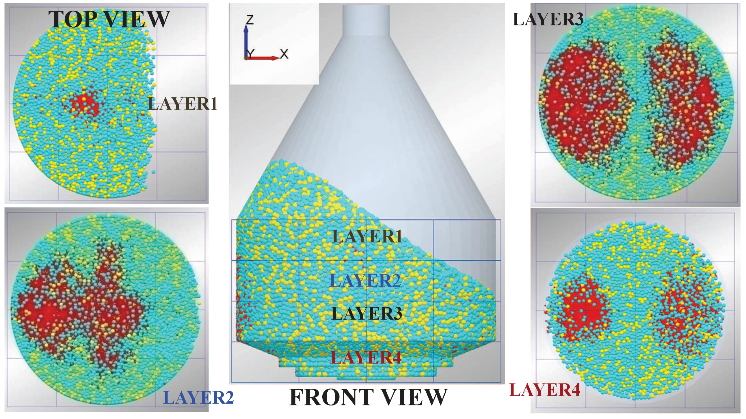Any unit operation is sensitive to certain critical process parameters (CPPs), and it has been shown in the previous studies [2,33] that the mixing efficiency changes significantly with the change in the conditions of these process parameters. A Cartesian coordinate system has been used for discretization of the blender into several zones. The geometry has been divided into four layers as seen in Figure 3. Each layer has been further divided into 16 grid bins. Therefore, the geometry has been divided into a total of 64 grid bins (4 × 4 × 4 in the x, y and z directions, respectively). It should be noted that a grid bin represents a zone or location inside the blender. When the model-based RSD of the blend composition is calculated, samples are collected from these zones for the RSD measurement. Therefore, changing the bin size will change the total number of zones inside the blender, which will in turn change the number of samples collected for the RSD measurement. In order to fix the bin size, the RSD has been calculated as a function of time by varying the bin size (which in turn changes the total number of bins), and the final bin size has been chosen in the range where the change in RSD between two bin sizes was not significant. Figure 3 and Figure 4 give a pictorial representation of the grid bins/zones inside the blender. It can be seen from Figure 3 that there are almost no particles or very few particles present in some of the grid bins. This is because a Cartesian coordinate system has been considered in order to discretize the cylindrical vessel. Therefore, these bins have been excluded from the RSD calculation so that spurious results are not obtained. 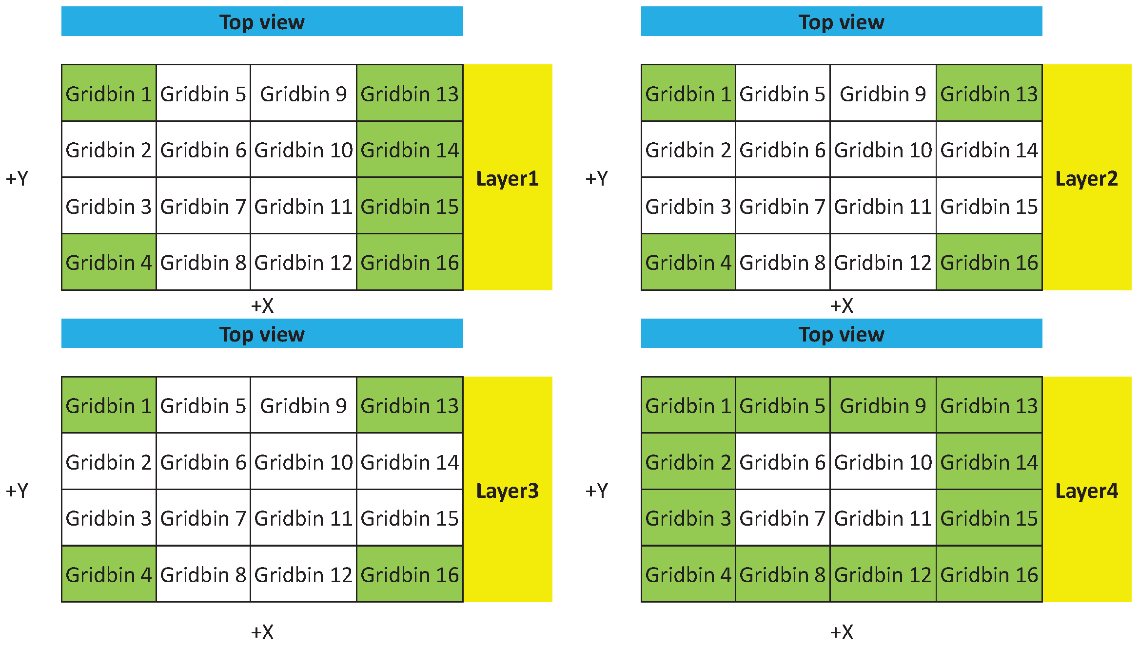Figure 4 presents the Cartesian grid bin representation of the four layers from the top view. It shows the excluded grid bins, which have been marked in green. The Grid Bins 6, 7, 10 and 11 in Layer 4 are all closest to the blender lid. Hence, the compositions from these four bins have been used to calculate the RSD at the lid.

Figure 5 represents the comparison between the overall RSD with respect to each material type, as a function of the number of revolutions, to their RSD in Layer 4 only (i.e., the near-lid region). RSD (for the i-th material type) has been determined based on Equation (4) as shown below. The overall RSD has been calculated by considering all of the grid bins excluding the ones highlighted in green, as shown in Figure 4. As explained above, samples collected from these grid bins have been used for RSD calculation. These RSDs represent instantaneous values as they are calculated from compositions in the grid bins at the end of a revolution.

$$RS{D}_i=\frac{\sqrt{\frac{{\sum }_{i=1}^{i=M}{(x_{avg}-x_i)}^2}{M-1}}}{x_{avg}}$$

(4)

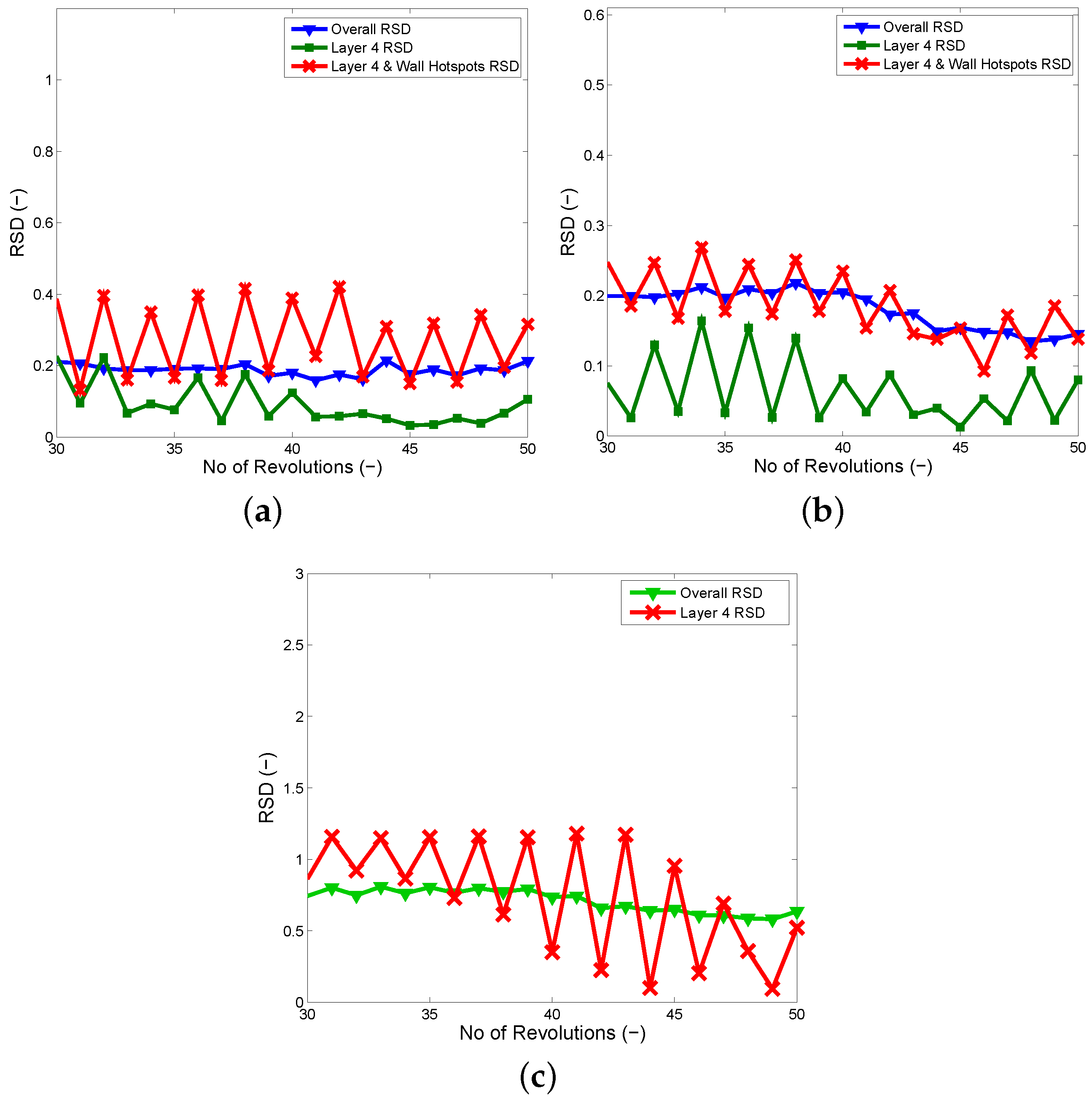
As mentioned, the blender has been divided into several bins, and samples for measurements have been collected from each of these bins. Here, $x_{avg}$ is the overall average fractional composition; $x_i$ is the fractional composition at the i-th bin; and M is the total number of bins. In other words, M is the total number of samples collected from the model for performing the RSD calculations. Figure 5a–c represents the comparison of RSDs obtained from the different locations (i.e., overall RSD, Layer 4 RSD and Layer 4 and wall hotspots RSD). The calculation of the overall RSD has been defined above. The Layer 4 RSD is the RSD at the blender lid. The meaning of ‘Layer 4 and wall hotspots RSD’ will be explained later in this section. The oscillations present are an inherent property of DEM simulation and have been observed previously in the literature [15]. As the powder particles can interact with each other and the geometry wall and move around the space in several different ways, based on the interaction parameters, contact angle, etc., oscillations in the output variables are often observed. The oscillations present in the overall RSD are much smaller in magnitude because the RSD has been computed taking all particles into consideration. However, from Figure 3, it can be seen that there is a mass of a few hundred particles present above Layer 1 when the blender is in the inverted position, which cannot be included in the calculation, as the discretization scheme does not allow it. Therefore, some particles are moving in and out of this mass (which changes the total number of particles considered for calculation) at every revolution. Therefore, the small oscillations are seen in the overall RSD. The oscillations present in the Layer 4 RSD are of higher magnitude because the RSD has been calculated for Layer 4 only, which is a small section inside the blender. A large number of particles can move in and out of this layer at every revolution, thus changing the total number of particles in Layer 4, which gives rise to the oscillations. It can be seen from Figure 5a,b that the RSDs from the compositions from the near lid regions are under-estimating the overall variability of API 1 and API 2 in the mixture. However, the mean values of the near lid RSD for each revolution give closer estimates of the overall variability for the extra granular phase compared to the other two components, as seen from Figure 5c. Overall, we can conclude that the measurements made near the lid are insufficient to capture the variability in composition of the blend.

It is important to note that the blend uniformity may improve when the ingredients are mixed for a longer period of time. The importance of mixing time has been discussed briefly in Section 4. The lower the RSD, the lesser is the variability in composition of the ingredients. If the ingredients are well and uniformly mixed over all of the zones inside the blender, there is still a possibility that the near-lid RSD will be able to represent the overall blend variability towards the end of the mixing time. However, these readings are not sufficient to estimate the dynamic variability of the blend, especially during the initial stages of mixing when the overall variability of the blend is high (as seen from Figure 5, as well). The information on dynamic variation is important (e.g., if a control loop needs to be designed in the future), which can be obtained easily from the model. For example, Godena et al. have highlighted the important steps involved in designing a batch process control system [34].

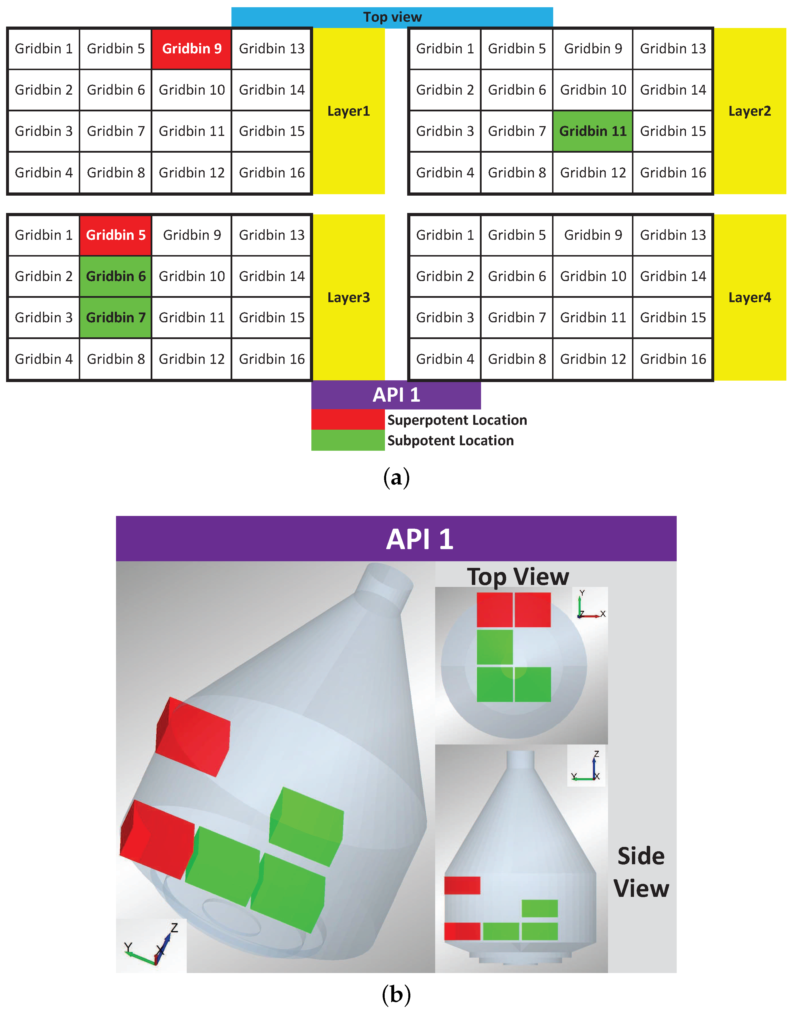
In order to obtain a better approximation of the overall RSD in the case of API 1 and API 2, there is a scope for identifying other sampling locations. The data from the additional sampling locations along with the near-lid readings could give a better estimate of the overall mixture variability. The RSD plots with the legend ‘Layer 4 and wall hotspot RSD’ in Figure 5a,b have been calculated after identifying the additional sampling locations, as has been detailed in this paragraph. In this study, the zones/bins with maximum and minimum fractional composition (with respect to the whole blender) have been identified at every revolution once the first 30 revolutions are complete (i.e., from 30th revolution to the 50th, a total of 21 revolution points). If a maximum or minimum composition has occurred in a particular bin more than three times (or at more than three revolution points), then that bin has been marked. The colors red and green stand for super-potent (maximum or more than the overall average composition) and sub-potent (minimum or less than the overall average composition) locations, respectively. 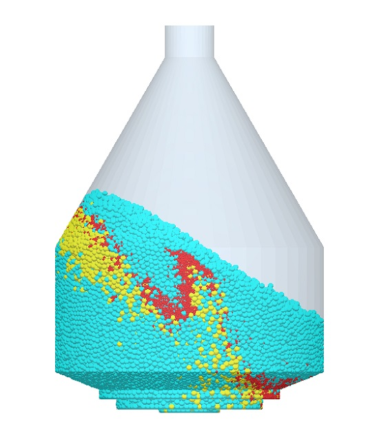Figure 6a,b shows the bin locations for API 1 in the Cartesian system and 3D representation, respectively. It can be seen that the super-potent spots are occurring towards the wall, and the sub-potent spots are occurring towards the center most of the times. 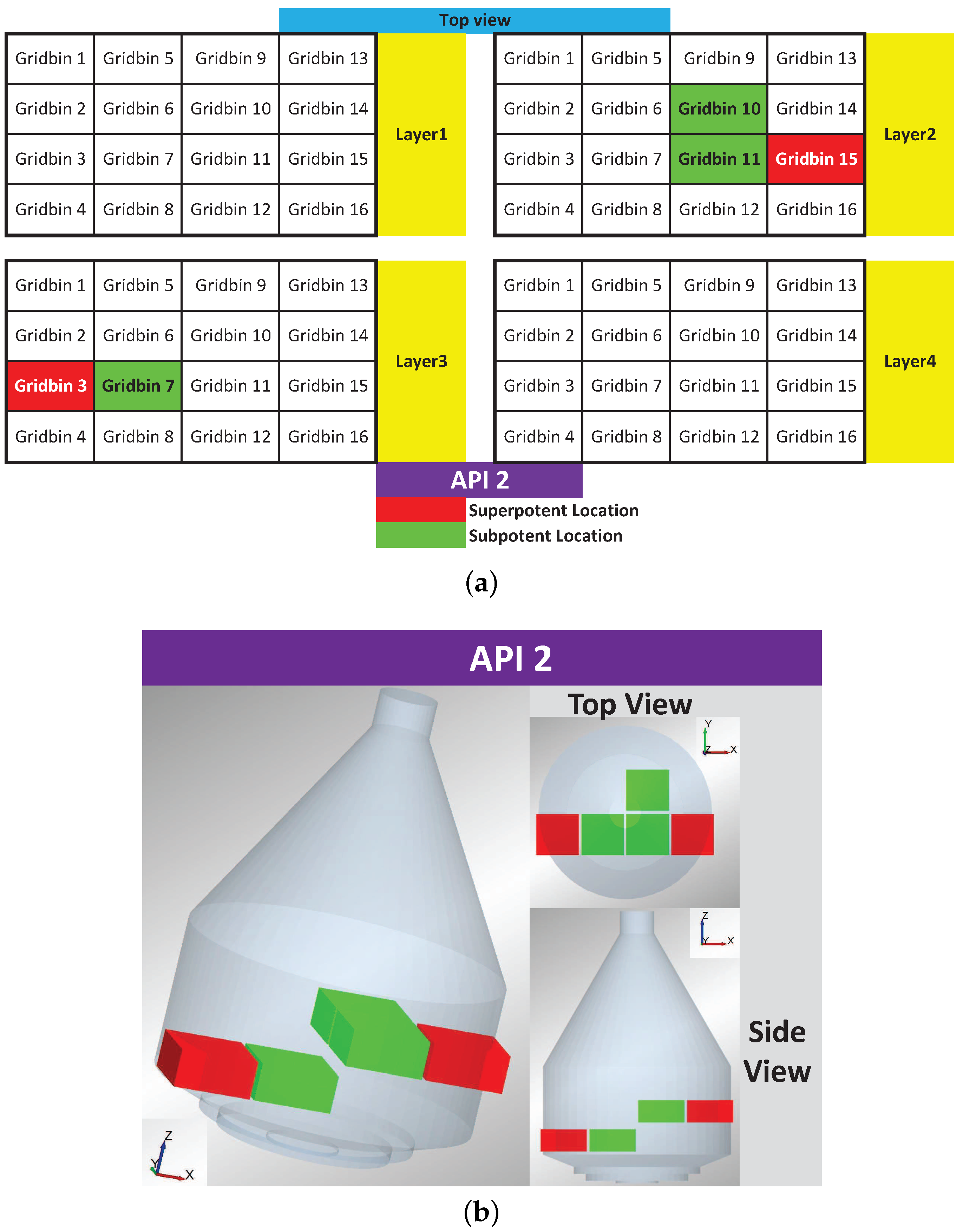Similarly, Figure 7a,b presents the bin locations for API 2 in the Cartesian system and 3D representation, respectively. A similar segregation pattern is observed in the case of API 2, as well. The zones identified in this study represent poorly-mixed regions. Thus, they can be potential sampling sites to enable better understanding of the blend composition. For each of these components, only the super-potent regions near the blender wall have been chosen as the additional sampling points due to the ease of data collection without interfering with the blend system. For example, one way to monitor the wall regions can be by drilling a hole on the equipment wall at the required location and installing a window and a sensor.

The additional sampling sites in the case of API 1 are Grid Bin 9 in Layer 1 and Grid Bin 5 in Layer 3. The additional sampling sites in case of API 2 are Grid Bin 15 in Layer 2 and Grid Bin 3 in Layer 3. The new RSD has been calculated by including the additional sampling data points along with the Layer 4 data and termed as ‘Layer 4 and wall hotspot RSD’. The new RSD has been compared in Figure 5a,b with the overall RSD. It can be seen from the plots that there is a good approximation, and the new RSD is not under-estimated when compared to the overall mixture RSD.

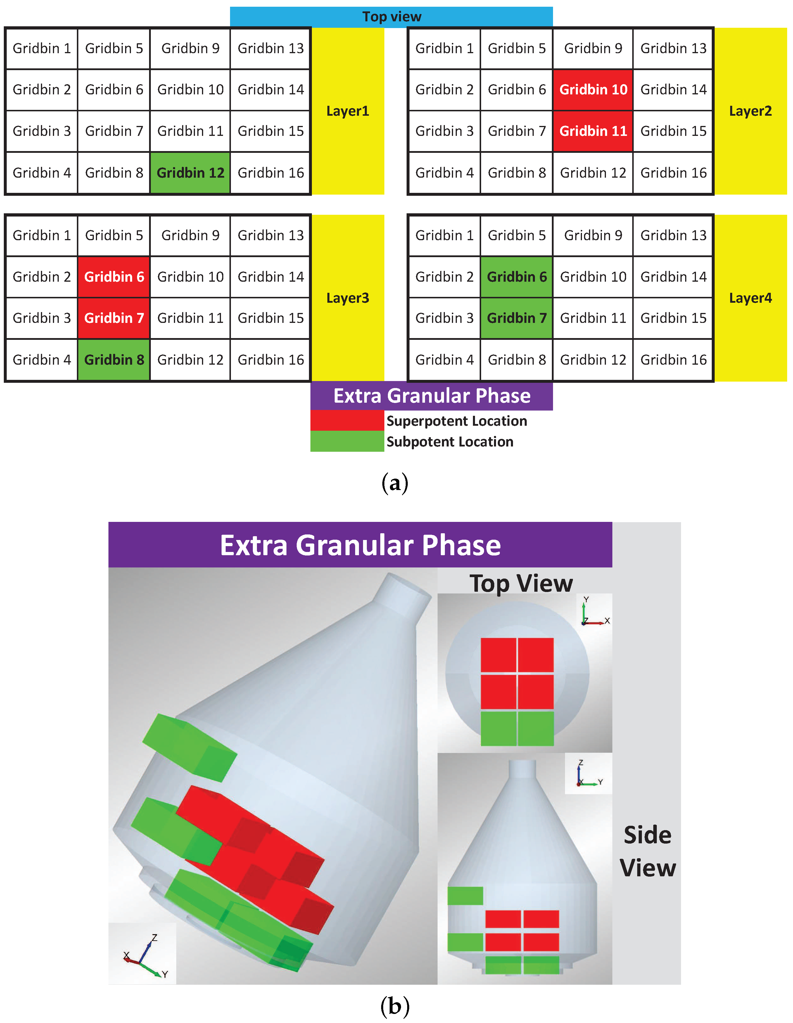
Figure 8a,b gives the bin locations for the extra granular phase in the Cartesian system and 3D representation, respectively. In the case of the extra granular phase, the super-potent spots occur towards the center, and the sub-potent spots occur towards the wall. This implies that the extra granular phase is forming a slowly-mixing segregated layer towards the center, which is away from the wall of the blender. Alexander et al. reported that the segregation pattern changes with the change in the blender RPM. For example, at a low blender speed, they observed that the smaller-sized particles form a separated band at the center surrounded by an outer band of large-sized particles, and the pattern is reversed when the blender speed increases [35]. In the present study, the blender RPM is low, and a similar observation of smaller particles segregated towards the center and larger particles towards the wall has been obtained. There is a possibility that similar observation can be made in the experimental setup, as well as in the beginning of the mixing operation; however, the segregated zones may go away with time when the mixing is complete.

The system is comprised of three types of materials, each consisting of particles with different sizes. As a result, the chances of observing segregation is high. Segregation effects are often seen in different powder handling operations as particles with different sizes and density often tend to form segregated layers, thus deteriorating mixing performance [36]. In order to quantify the extent of segregation of the three material types, the intensity of segregation (I) has been determined based on the equation below (Equation (5) [37]).

$$I=\frac{{\sum }_{i=1}^{i=M}{(x_{avg}-x_i)}^2}{M{x}_{avg}(1-x_{avg})}$$

(5)

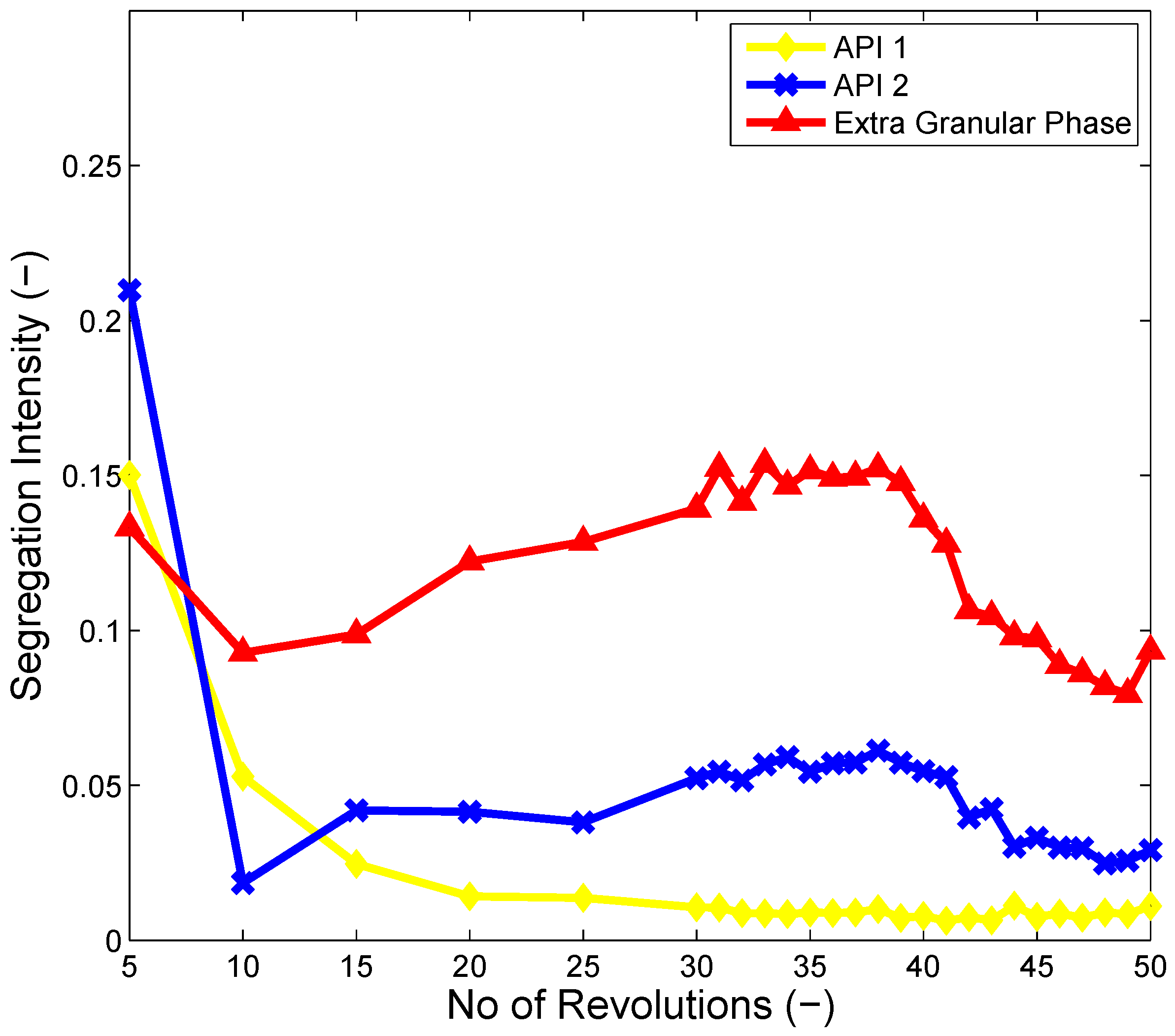
Figure 9 gives the intensity of segregation as a function of the number of revolutions. It can be seen that the segregation intensity of the extra granular phase is the highest. The API 1 and API 2 particle sizes used in the simulation are comparable (the size ratio between the two is 1:1.05), but the extra granular phase particles are much smaller (approximately 2.5-times) than the other two. As a result, the extra granular phase forms a segregated layer, which is mixing slower compared to the other two material types, since the segregation intensity of the extra granular phase is comparatively high. It is also seen that the extra granular phase is mainly concentrated towards the center and is mixing very slowly. Therefore, it has a high variability throughout the mixture. This may be the reason why the near-lid measurements are able to capture the overall RSD of composition for the extra granular phase. On the other hand, API 1 and API 2 have certain well-mixed and poorly-mixed zones due to which the measurements at the blender lid are not able to capture the overall RSD of these two entities. The segregation pattern is a strong function of the fill level, blender RPM and particle properties (i.e., size and shape). In the previous studies, it has been observed that the segregation pattern of differently-sized and -shaped particles varies with the change in the processing conditions [38,39].

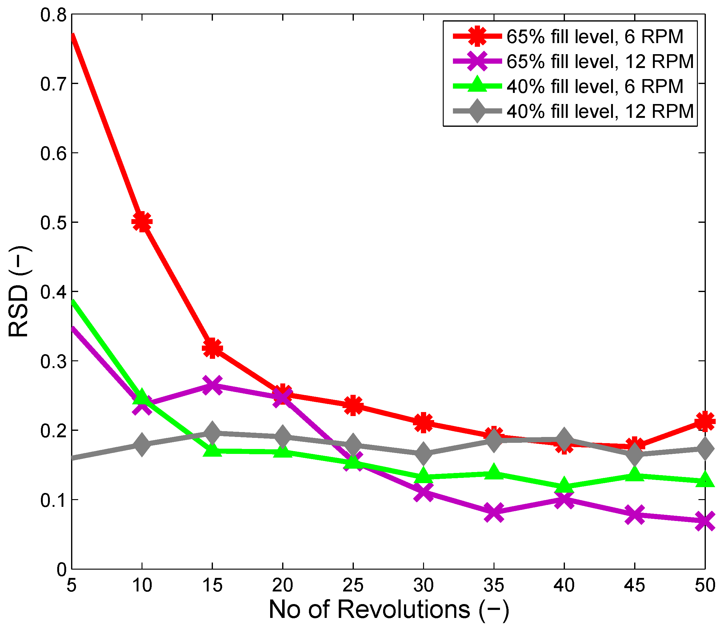
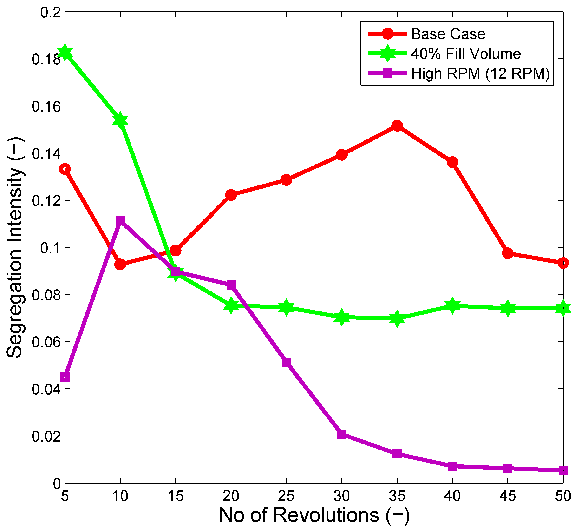
Segregation of a component during mixing is not desired, hence the model has been used to evaluate the changes that need to be made in the processing conditions such that the segregation effect is lowered and a better quality blend is obtained in lesser operational time. Certain process parameters critical to mixing (e.g., fill level and RPM) have been varied, and their effect on the mixing dynamics has been studied. This will help determine how these CPPs can be tuned in order to reduce the segregation intensity and also enhance the mixing efficiency, which will allow the slowly-mixing center consisting of the extra granular phase to go away. Two more cases have been run where the fill level has been reduced to 40% (total number of particles simulated is 125,000) in one, and the blender RPM has been increased to 12 in another one, keeping all other simulation parameters the same as the base case. Figure 10 shows the change in intensity of the segregation of the extra granular phase with the variation in RPM and fill level. It can be seen from Figure 10 that the segregation intensity reduces with the increase in RPM or the decrease in fill level. As the RPM increases, it increases the convective transport of the particles, thus resulting in a fast mixing, which enhances the mixing efficiency. With the decrease in fill level, the particles have enough space to travel from one location to another, which aids in particle transport. In the bin blender simulations, it has been noticed that the mixing of the materials takes place mainly near the free surface of the batch as the blender rotates. Therefore, at a higher fill level and low blender RPM, the segregated layer of the extra granular phase at the center is not getting enough space and energy to move around. However, as the fill level is reduced and the blender RPM increased, a better mixing of the extra granular phase is being achieved. As considerable effects of these process parameters have been observed on the mixing dynamics, therefore a separate study has been conducted to understand the influence of the various process parameters (as detailed in Section 4). It is important to observe the effect of the different process parameters as this will help to arrive at an optimal processing condition.

The developed model has been compared with some of the experimental work done by other researchers on studying the segregation patterns in tumbling blenders. The results of the the model qualitatively match the observations made in these works. For example, Alexander et al. carried out an experimental study on the segregation patterns in a tumbling V-blender [40]. They observed that the smaller particles occupy the interior, whereas the bigger particles tend to occupy the exterior space. The reason behind this observation as outlined by the authors is that the big and heavy particles tend to travel more rectilinearly than the smaller and lighter particles in a transverse forcing field. As a result, the smaller particles can follow trajectories with higher curvatures and tend to occupy the interior of a curved flow path-line when compared to the bigger particles. Similarly Alizadeh et al. [41] used a radioactive tracking method in order to investigate the segregation pattern in tumbling blenders. They used differently-sized glass spheres in their experiment and observed that the smallest size of glass spheres (3 mm in diameter) forms a core along the material rotation axis, and they are surrounded by the larger spheres (5 mm and 6 mm diameter). Porion et al. [42] used a nuclear magnetic resonance (NMR) imaging technique to study the mixing and segregation in a 3D batch blender (shaker-mixer) and observed a similar segregation pattern based on the particle size (i.e., the large coated beads segregated to the outer part of the cell in their experiment). The results obtained from this model also depict that the larger particles (API 1 and API 2) tend to occupy the outer volume of the blender, and the smaller particles (extra granular phase) form a slowly-mixing core. This shows that when compared to the other experimental observations available in the literature for different types of tumbling batch blenders, the present model shows a good qualitative agreement.

Effect of Process Parameters on Blend CQAs

As identified in the previous studies [43], the main design and process variables that affect the mixing dynamics are geometry, the design of the blender and the mixing mechanism, blender size, fill level, rotation speed of the blender (RPM), material loading order and material properties of the raw materials. In the present study, the design parameters or equipment geometry and the material properties are fixed. Therefore, the process variables (i.e., the fill level, loading order and blender RPM) have been varied in order to determine their effect on the mixing performance of this particular system. This study will help to demonstrate how this model can be used for process design and to determine the sensitivity of the process parameters. The RSD has been calculated every five revolutions, based on the RSD of API 1, since this is the API of interest. 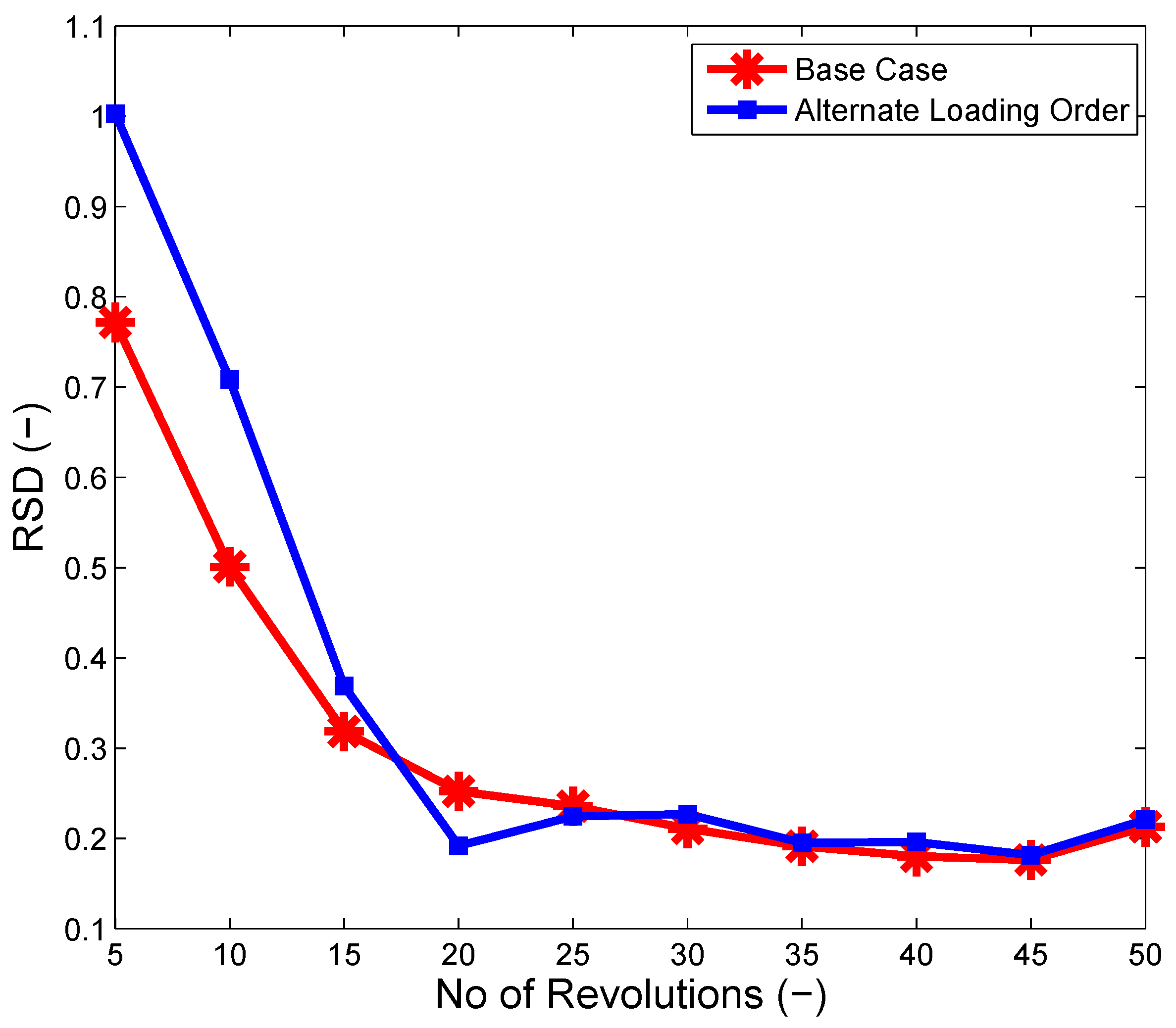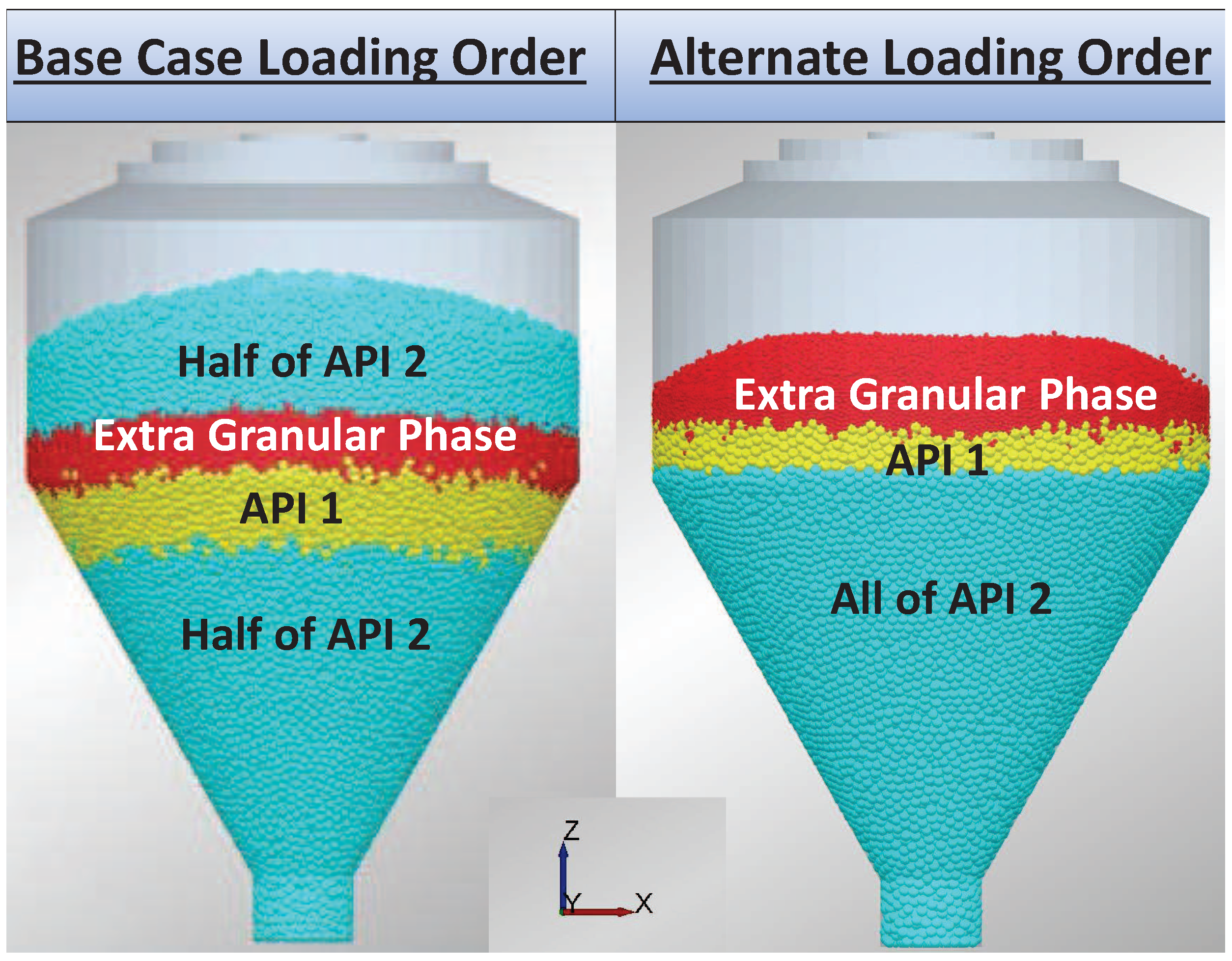Figure 11 shows the two different loading orders (i.e., base case loading order and alternate loading order). In the alternate loading order, materials have been added as all API 2 followed by all API 1 followed by all of the extra granular phase. Figure 12 presents the plot of RSD with respect to API 1 with different loading orders. It has been seen that the effect of the loading order is the least in the present case as the average change in RSD with the alternate loading order is 0.5% only. Therefore, loading order has not been considered for further investigation, as it has been found to be the least sensitive process parameter for the present system.

Two process parameters (fill level, blender RPM) have been studied and two levels of each have been considered. The two levels for the fill level are high 65% and low 40% and blender RPM are low 6 RPM and high 12 RPM. Following a factorial design, $2^2=4$ simulation conditions were obtained. These conditions are as shown below (it should be noted that all other input parameters are the same as defined in Section 3.3):

• Case 1: Blender RPM = 6 and fill level = 65% (which is the base case)
• Case 2: Blender RPM = 6 and fill level = 40%
• Case 3: Blender RPM = 12 and fill level = 65%
• Case 4: Blender RPM = 12 and fill level = 40%

Figure 13 illustrates the RSD of API 1 as a function of the number of revolutions for the four different conditions as listed above. The RSD decreases with the reduction in the fill level and the increase in the blender RPM. As highlighted previously, this occurs due to the increase in convective particle transport as the RPM increases. As the blender RPM increases, it imparts more energy to the particles, which in turn increases their kinetic energy. As a result, the particles are mixed better. The RSD increases with the increase in the fill level because with the increase in the fill level, lesser free space is available for particle movement, which hinders the particle transport. RSD decreases over the number of revolutions for Case 2 (blender RPM = 6 and fill level = 40%) and Case 3 (blender RPM = 12 and fill level = 65%) when compared to the base case. However, for Case 4 (blender RPM = 12 and fill level = 40%), the RSD is the least (among all four cases) until the 12th revolution, after which the RSD starts increasing and approaches the base case RSD at the 35th revolution. One explanation for this observation is that due to a high RPM and low fill volume (i.e., less amount of raw materials), the ingredients are mixed comparatively faster (i.e., by 12 revolutions), and mixing beyond 12 revolutions causes segregation. The particles could be undergoing a spatial re-arrangement due to the contact and body forces acting on them, which may lead to a segregation of the previously well-mixed blend. Therefore, mixing time is also an important factor to be considered in the case of a batch mixing operation. Mendez et al. illustrated the effect of mixing time on the homogeneity of the drug product in the mixture using a V-blender and observed that this parameter can be used to control the mixing operation on a large scale during batch production [44]. While studying the optimum mixing time for a mixture of lactose and colloidal silicon dioxide, Sindel et al. also observed that the variability of the mixture reduces with time initially and reaches an optimum homogeneity, then starts increasing again [45].

Mixing time is an important factor in deciding the blend quality [46] in the case of the batch mode of operation. Optimal mixing time will change if the CPPs are varied. It can be adjusted to obtain the desired product quality. However, in this work, a study on the mixing time has not been conducted, as the present DEM model is computationally intensive. However, the same framework can be used to study the effect of mixing time. In order to run the model for a longer time period, it is suggested that a reduced order model (ROM) is developed from the DEM. An ROM is faster and will have the details of the DEM, as well [47]. The other option is to use parallel computing tools to speed up the simulation.

5. Conclusions

A mathematical model has been developed based on the DEM methodology for an industrial batch bin blender, where three different types of materials (API 1, API 2 and the extra granular phase) are mixed. The results reported in this work have been obtained from the model-based analysis. The model has been calibrated to represent the materials used in the real experimental setup and used to evaluate the effect of the current processing conditions on the mixing efficiency. The model has been used to determine if the composition data near the blender lid region are capable of predicting the overall blend variability. It has been seen after conducting this qualitative model-based study that the composition data from only the near-lid zone do not provide a dynamic representation of the overall variability in the composition of the entire blend. Therefore, additional sampling sites have been identified so that a good approximation can be obtained. A segregation study has been conducted that highlights the segregation pattern of the different materials being mixed. It is seen that the extra granular phase forms a slowly-blending segregated layer towards the center. Alternate processing conditions (i.e., how the CPPs can be adjusted) have been suggested for counteracting the segregation effect seen for the extra granular phase. It is seen that the intensity of segregation decreases considerably with the increase in blender RPM and the reduction in fill volume. It is seen that the loading order is the least sensitive in this particular case, whereas fill volume and blender RPM have high sensitivity towards the blend product quality. A separate study on the mixing time has not been conducted in this study, but it has been illustrated that determining the optimal mixing time is important, and it will change with the change in the processing conditions. The results obtained from this model have been shown to agree with the previous studies reported in the literature [2,33,43]. The observations obtained from the model in the present study represent the dynamic variation of the CQAs right from the process startup. Even though this model simulates a case with large-sized particles, the DEM material properties have been calibrated in order to capture a certain important actual property (i.e., angle of repose). It has been demonstrated that information obtained from this model can help with qualitative understanding of the mixing operation. An experimentally-calibrated and -validated model developed from first-principles can be used to mimic the real system, identify the processing issues present in the real system and improve the mixing efficiency so that better quality products can be obtained. This work presents the initial steps in developing such a model-based framework. The next step is to validate the model with the experimental observations and use it to study the effect of equipment design parameters and different mixing mechanisms.