Numerical Aspects of Data Reconciliation in Industrial Applications
by
 ,
,
Maurício M. Câmara
1, 
Rafael M. Soares
1,
Thiago Feital
1,2, 
Thiago K. Anzai
3,
Fabio C. Diehl
3,
Pedro H. Thompson
3 and
José Carlos Pinto
1,* 1
Programa de Engenharia Química/COPPE, Universidade Federal do Rio de Janeiro, Cidade Universitária,CP 68502, CEP 21941-972, Rio de Janeiro, RJ, Brazil
2
OptimaTech, Rio de Janeiro, RJ, CEP 21941-614, Brazil
3
Centro de Pesquisas Leopoldo Americo Miguez de Mello–CENPES, Petrobras–Petróleo Brasileiro SA, Rio de Janeiro, RJ, CEP 21941-915, Brazil
*
Author to whom correspondence should be addressed.
Processes 2017, 5(4), 56; https://doi.org/10.3390/pr5040056
Submission received: 28 August 2017
/
Revised: 25 September 2017
/
Accepted: 29 September 2017
/
Published: 3 October 2017
(This article belongs to the Collection Process System Engineering for More Efficient Power and Chemicals Production)
Abstract
:Data reconciliation is a model-based technique that reduces measurement errors by making use of redundancies in process data. It is largely applied in modern process industries, being commercially available in software tools. Based on industrial applications reported in the literature, we have identified and tested different configuration settings providing a numerical assessment on the performance of several important aspects involved in the solution of nonlinear steady-state data reconciliation that are generally overlooked. The discussed items are comprised of problem formulation, regarding the presence of estimated parameters in the objective function; solution approach when applying nonlinear programming solvers; methods for estimating objective function gradients; initial guess; and optimization algorithm. The study is based on simulations of a rigorous and validated model of a real offshore oil production system. The assessment includes evaluations of solution robustness, constraint violation at convergence, and computational cost. In addition, we propose the use of a global test to detect inconsistencies in the formulation and in the solution of the problem. Results show that different settings have a great impact on the performance of reconciliation procedures, often leading to local solutions. The question of how to satisfactorily solve the data reconciliation problem is discussed so as to obtain improved estimates.
1. Introduction
Reliable data is essential to any industrial process. From process operating to planning and scheduling, it is used to support decisions that affect product quality, plant profitability, and plant safety. It has implications in environmental and legal issues, such as pollution monitoring by state agencies. In production accounting, it is involved in the quantification of significant issues, such as trade and custody transfer and process inventories. However, especially in industrial environments, obtaining reliable information during daily operation is not a trivial task.
Measurements of process variables, both on- and off-line, are subject to random errors (noise), such as natural disturbances, sampling errors, unreliable instrument readouts and laboratory analyses inaccuracies, and nonrandom errors, such as sensor bias or sensor failure (gross errors) [1]. Random noise may also be the outcome of other effects, such as high-frequency pick-up, low resolution, and errors in transmission and conversion (including A/D and D/A conversion) [2], usually attributed to the irreproducibility of the measurement devices [3]. Consequently, the collected data generally do not even satisfy basic process constraints, such as the mass and energy balances. Inaccurate process data could result in misleading or inaccurate conclusions, thus leading to poor decisions that can adversely affect many plant functions. Thus, to reduce the impacts of measurement errors in plant measurements and to increase the value of data accessible through implemented data management systems, data rectification should be employed [4].
Data rectification is a collection of techniques for correcting data and is comprised of different steps, such as variable classification, gross error detection, parameter estimation, and data reconciliation [5]. At its core, data reconciliation (DR) is a model-based technique that reduces measurement errors by making use of redundancies in process data. It aims at estimating the true state of the plant based on the adjustment of process measurements in order to satisfy a set of constraints, which is accomplished by minimizing some sort of deviation between corrected and observed plant values. Unlike other filtering techniques, DR makes explicit use of the process model so that reconciled estimates are consistent with the known relationships between process variables as defined by the constraints, as well as being expected to be more accurate than the measurements [6,7].
Data reconciliation may also be used as an effective monitoring tool, producing estimates for non-measured variables and process parameters. In many systems and applications, parameter estimation is the step after data reconciliation, where reconciled values of the measured variables are used to estimate/update model parameters [8,9,10]. Nonetheless, procedures for data reconciliation with simultaneous parameter estimation (DRPE) are equally valid and efficient [11,12,13,14,15]. It is worth noting that measurements of independent variables are typically assumed to be free of error. In this context, DR may also be applied when both dependent and independent variables contain errors, which some authors label as an error-in-variables method (EVM) [16,17]. EVM provides both parameter estimates and reconciled data estimates that are consistent with respect to the model. Besides, techniques for joint data reconciliation and parameter estimation with simultaneous gross error detection have emerged based on robust statistics, which are especially important for on-line industrial applications [18]. Many robust estimators have been proposed to reduce the effect of gross errors and yield less biased estimates [19,20,21,22,23]. Alternative approaches to gross error detection involve the use of principal component analysis [24,25], cluster analysis [26], artificial neural networks [27], and robust [28] and correntropy [29] estimators. More recently, a practical DRPE methodology for process systems with multi-operating conditions along with a correntropy estimator [30] and a unified framework for applying principal component analysis (PCA) and DR [25] have been presented.
The literature regarding data reconciliation is comprised of a vast number of works and good compilations of the techniques available and can be found in the open literature [28,31,32] as well as the comprehensive books [5,33,34,35,36]. Beginning with steady-state problems with linear constraints for the case when all variables are measured [37], advances in optimization techniques have allowed more complex formulations addressing steady-state nonlinear [19,38,39,40,41], dynamic linear [42,43,44] and dynamic nonlinear [15,26,45,46,47] data reconciliation problems. In each of these formulations, the process model, represented by the (differential) algebraic equation system, is a constraint of the mathematical programming model representing the estimation problem, where the solution of the system’s equations is required to solve the optimization problem.
Largely applied in most modern process industries, DR is commercially available in software tools such as Aspen Advisor (Aspen Technology, Inc., Bedford, MA, USA), VALI (Belsim, Awans, Belgium), VisualMesa (Soteica, Houston, TX, USA), SimSci DATACON (Schneider Electric Software, Lake Forest, CA, USA, LLC), and Sigmafine (OSIsoft, San Leandro, CA, USA), among others [48]. In addition to in-house systems [49,50,51], these tools can be used to reconcile flow, temperature and composition measurements to satisfy material and energy balances around each unit in a process plant, as well as to estimate parameters [52,53,54]. Furthermore, the increasing availability and decreasing cost of high performance computers have allowed the implementation of more robust and complex applications, where reconciled measurements are used in on-line applications such as performance monitoring, process control, and real-time optimization [55,56,57].
Given the importance of DR techniques, its expressive body of knowledge and its availability in commercial tools, detailed descriptions of data reconciliation procedures and its use in actual industrial applications are relatively scarce in the open literature. This apparent discrepancy may be partially attributed to proprietary reasons and confidential constraints. Works related to industrial DR implementations are mainly concerned with the challenges in obtaining a precise mathematical representation of the process given the information available. They typically concentrate on developing procedures and computation strategies to new systems, which most often involve formulating the DR problem based on a rigorous process model and solving it using a typical optimization algorithm suitable for high-dimensional mathematical programming problems, as well as more robust gross error detection schemes. Although they are of undeniable technical value, the implementation and advance of on-line DR applications require the choice of the most suitable implementation setting.
Indeed, the availability of a precise process model and a suitable set of measured variables are not enough for adequately solving the DR problem. Few studies present more detailed analyses for settings regarding distinct areas, such as problem formulation [4,28], solution method [12,58,59] and approach [60,61], optimization algorithm [54,62,63,64], and solving strategies [23]. Distinct settings, even those represented by minor differences, may present different performances but commonly are not discussed. Nevertheless, they should be analyzed during the design of a DR application trying to answer whether the optimization problem is being satisfactory solved. Although DR generates benefits, it can have strong negative effects when some hypothesis is violated or the procedure does not find a feasible solution, and using reconciled data could yield worse results than using the measurements directly [65,66,67].
In this work, we aim at providing a numerical assessment on the performance of different settings for solving nonlinear steady-state data reconciliation. We show that different settings have a great impact on the performance of DR procedures and that an adequate setting must be found. Problem formulation, regarding the presence of estimated parameters in the objective function, and thereby solution approach, either sequential or simultaneous, are considered when applying nonlinear programming (NLP) solvers as the solution method. We devote attention to investigate the impact of methods for estimating objective function gradients required by deterministic optimization algorithms, which is generally overlooked in DR studies and applications. In this work, the interior-point (IP) algorithm is applied. The performance of a hybrid algorithm combining the metaheuristic algorithm particle swarm optimization (PSO) and IP is also evaluated and compared. As a known variable affecting the performance of optimization algorithms, we analyze the influence of the initial guess in the solution of the DR problem. The assessment includes evaluations of solution robustness, constraint violation at convergence, and computational speed. In order to better control the results, only simulation data is used in the study and gross error detection is not considered in the scope of this work. The study is based on simulations of a rigorous and validated model of a real offshore oil production system. The process model is available from a reliable proprietary simulator largely used at Petrobras. It is important to emphasize that very few works focus on the use of data reconciliation procedures on oil production systems [2].
The remainder of this article is organized as follows. Section 2 presents a brief overview of data reconciliation in industrial applications. Section 3 describes the offshore oil and water production systems for which the study is based on, and also details the simulation experiments conducted for assessing different settings for solving nonlinear DR. The results are presented and discussed in Section 4, and finally this work is concluded in Section 5.
2. Overview of Data Reconciliation in Industrial Applications
2.1. Problem Formulation
The essence of data reconciliation is that, given the measurements from the plant, we want to estimate the process state, which satisfies the known relationships between process variables as defined by the (first principles) process model. The actual estimated condition of the process is obtained as the solution of
where is the objective function and is the function vector representing the known inequality process constraints, where knowledge of the parameters is assumed . The vector of measured process variables consists of output process variables (), but may also include process inputs (), and is defined by the measurement mapping matrix , where if variable j is measured and the measured value is located in , such that .
Depending on the nature of the process model equations, the DR problem may be either linear or nonlinear, and either static or dynamic. As shown in Table 1, most of the applications found are related to steady-state nonlinear data reconciliation. In this context, considering nonlinear steady-state DR problems, process model equations are conveniently represented by
An important part of DR problem formulation is the definition of the objective function . It might be based on a deterministic approach following classical regression techniques [28], being defined, for example, as a weighted least-squares estimator (WLS) [110]:
where is the weighting matrix.
Another approach to formulate the problem and define the objective function is based on a probabilistic framework utilizing the maximum likelihood method, for which the measurements of are assumed to contain random errors so that
where is the vector of measurement errors. The advantage of applying the maximum likelihood method is that it gives efficient (or minimum variance bound) and unbiased estimates, which means that estimates have the lowest theoretically attainable variance, and an expected value equal to the true value of the variable, respectively [111]. In this method, the likelihood function () corresponds to the joint probability distribution of measured variables as a function of the estimated variables/parameters. Thus, assuming measured variables are statistically independent, the objective function is the product of the individual probability density functions p of the measured variables, i.e.,
where is the variance of variable i. The maximum likelihood estimate is the value for which the likelihood function attains its maximum while satisfying equality and inequality constraints. Nonetheless, both regression and maximum likelihood approaches are closely related when the measurement error is uncorrelated among different measurements and is normally distributed with zero mean and positive definite covariance matrix , . For such a case, the likelihood function in Equation (4) may be simplified to a quadratic function, so that the maximization of this simplified function is equivalent to minimizing Equation (2) with [112,113]. Formulations of the DR problem typically follow Equation (1) with a WLS estimator supported by the (implicit) assumption of independent and normally distributed measurement errors, resulting in the following constrained nonlinear program
Equation (5) is easily extended to a DRPE problem by the inclusion of process parameters (or a subset of it) in the set of decision variables.
To deal with deviations from this conventional normal assumption, as is the case when data sets contain gross errors and outliers, gross error detection (GED) schemes have been proposed, such as the simultaneous approach for data reconciliation and gross error detection. This technique is based on robust statistics and consists on finding estimators (i.e., an objective function) whose mathematical nature, especially its influence function, is insensitive to deviations from the ideal assumptions on errors, giving less weight to the contribution of large errors in the estimation problem [4,21]. The expected result is a reduced effect of the eventual gross errors present, yielding less biased estimates. However, the use of robust estimators do not guarantee efficient and unbiased estimates since they will still be dependent on the distribution structure of the measurement errors according to maximum likelihood principles. In this context, a generalized robust data reconciliation approach has been proposed [114].
Even with advanced alternatives, the predominant estimator among industrial applications for plant-wise use is the WLS, where weights either follow the maximum likelihood method or are user defined according to some (heuristic) rule following the regression approach. In the former, the statistical framework for DR still requires the knowledge of the error covariance matrix , which depends on several aspects including sensor characteristics, amplifier, cable links, and digitizing circuits. Usually the variances are unknown but can be estimated by historical data, assuming .
Few cases do not follow the maximum likelihood method when defining the estimator. In the reconciliation phase of the On-line Reconciliation and Optimization (ORO) package described by Bussani et al. [71], DR is achieved by minimizing the weighted sum of squared residuals between the measured and calculated variable values normalized by measured values. In addition, some applications formulate the DRPE problem considering process parameters along with measured variables in the objective function. In an application for the gas separation system of a petroleum refinery, Piccolo et al. [13] included in the objective function estimated efficiencies of both de-ethanizer and debutanizer columns and debutanizer reboiler duty, which were determined in the same DRPE problem as estimated parameters. Similarly, Câmara et al. [67] reported the presence of a load characterization parameter in the objective function for the DRPE of a crude oil distillation unit.
2.2. Solution Methods
Different solution methods have been employed in industrial DR applications. The methods are problem-dependent and often exploit some features of the problem in order to achieve fast and efficient calculations.
When the resulting mathematical programming problem is a constrained least squares estimation with either linear or bilinear model constraints, analytical solutions and specific iterative procedures have been used [56,69,74,85]. Nonetheless, as more relations apart from overall material balance equations are required for rigorous process models, as well as variable bounds and feasibility constraints, the use of such methodologies is limited. In addition, the development of analytical solutions for linear and bilinear problems in the context of real applications could also be motivated by computational and programming limitations, which has changed remarkably with the increased availability and reduced cost of high performance computers.
In the absence of inequality constraints , the solution of nonlinear DR problems have been achieved by the use of the Lagrange multipliers method [59,70,86], where the partial derivatives for the Lagrangian of the DR problem are set to zero and the resulting system of equations is solved by any simultaneous equation solver, or by the method of successive linearization [12,58,59,76]. In the later, linear approximations to the nonlinear constraints are obtained by a Taylor series expansion about the previous iterate and a series of linear data reconciliation problems is solved until a solution satisfying the nonlinear constraints is obtained. Each intermediate solution is the optimal point for the linear constraints. Successive linearization provides relative simplicity and fast calculation, although it cannot handle variable bounds and it may fail to converge [36,58].
The most widely used method for solving nonlinear DR problems, such as that of Equation (5), consists of the application of well established, general purpose NLP algorithms. Indeed, several works have demonstrated that using NLP instead of successive linearization remarkably improved reconciliation results [115,116], so that nonlinear programming techniques have emerged as the most efficient. This method allows a general nonlinear objective function, such as robust estimators, and can explicitly handle inequality constraints. Inequality constraints, such as variable bounds, are generally required in the DR model to guarantee feasible estimates, e.g., nonnegative estimates for flows or compositions. Furthermore, in addition to steady-state DR, methods that apply NLP solvers are also used in the solution of dynamic optimization problems, as those resulted from nonlinear dynamic DR [15,83]. Thus, the NLP method is able to tackle a complete formulation of the data reconciliation.
Islam et al. [58] tested the three methods in a data reconciliation package for an industrial pyrolysis reactor. However, the discussion is limited to the influence of the initial guess in each one. It was observed that initial starting values far from the steady state values caused the successive linearization method to fail, converging to incorrect steady-state values. The NLP method employing successive quadratic programming (SQP), in turn, required a large computational time to get a comparable result but worked well in all cases with upper and lower bounds for all the reconciled variables. The use of SQP in the absence of variable bounds was not reported. Weiss et al. [12] have also evaluated these three methods of solving data reconciliation on an industrial pyrolysis reactor. The authors have observed similar results among the methods, which provided encouragement to the use of successive linearization since the large computational time required by the nonlinear method could not be justified. However, similar results among these methods is not observed in other works. In the report of Christiansen et al. [76] in applying DR to industrial synthesis gas preparation, successive linearization was applied only when the basic material balances were considered. For the use of a more rigorous model including the energy balance, as well as if it is desired to investigate the plant over a period of time, the NLP method was used employing a SQP algorithm with bounds on the independent variables.
Both the Lagrange multiplier and NLP methods were evaluated by Eksteen et al. [86] in the DR for an open arc smelting furnace. Systematic biases have been observed in the results, being larger when the Lagrange multiplier method was used. However, this comparison is not fair enough since the methods were not evaluated for the same DR formulation, where the Lagrange multiplier method solved the minimization of the variance weighted closure residuals of the mass balance equations, and the NLP method solved the minimization of the weighted sum of squared errors. In other work, the Lagrange multipliers and the successive linearization methods were employed for solving nonlinear DR on a coking plant based on a components balance and total flow rates balance [59]. It is argued that successive linearization has the advantage of relative simplicity and fast calculation and that, in general, the Lagrange multipliers method tends more frequently to shift the reconciled values in a biased direction.
Even with the increased availability of high performance computers, dealing with the large number of decision variables remains a challenge when using NLP in industrial applications, as well as the nonlinear and non-convex nature of the objective function, process model and other constraints. It has been observed that some NLP algorithms become inefficient when the number of degrees of freedom are large [117,118], and the dimension of the DR problem for large-scale process models can preclude regular optimization techniques from correctly solving the problem [23]. As a result, many authors have proposed either decomposition approaches as a solution strategy to overcome this difficulty when employing standard NLP solvers or optimization algorithms tailored for process applications with many degrees of freedom.
2.3. Solution Strategies
The most straightforward strategy for solving the nonlinear DR problem is to use nonlinear programming to estimate parameters and reconciled variables simultaneously. However, when the dimension of the problem significantly impairs the use of standard NLP algorithms, decomposition approaches may be used, which divide the original problem in multiple estimation problems of reduced dimensions.
Rod and Hančil [119] proposed an iterative algorithm that separately evaluates parameters and independent variables. Reilly and Patino-Leal [120] used a method in which the data reconciliation is nested within the parameter estimation step. Doví and Paladino [121] presented a constrained variation algorithm in which the dependent variables are eliminated by solving the model equations and thus eliminating the necessity of simultaneously iterating both parameters and true values of the measured variables but requires the second derivatives of the model. Kim et al. [16] compared three strategies for the nonlinear EVM problem, namely, simultaneous parameter estimation and data reconciliation, two-stage EVM, and nested EVM, in terms of computer time and converged parameters and reconciled variable values for test problems from the literature. When evaluating these strategies, a generalized reduced gradient (GRG) and a SQP algorithm were used. As observed in their results, the two-stage nonlinear EVM outperformed the other alternatives and was reported as the only recommended solution strategy.
Regarding industrial DR applications, the predominant strategy is the direct solution of only one nonlinear DR problem, where parameters are estimated along with reconciled variables (DRPE/EVM) when present. Quelhas et al. [66], however, brought attention to the fact that the estimation problem must be carefully designed. Dealing with a two-step RTO applied to an industrial ethylene production plant, it is shown that the typical trajectories of the estimated heat transfer coefficients indicate that some of the model parameters are not estimable when the parameter estimation is performed independently and simultaneously with the data reconciliation procedure, which might be due to correlation with other parameters and process data or because they do not affect the objection function significantly. Other strategies are briefly discussed below.
By establishing that the complexity of large dimension optimization problems can be reduced by performing a partition of the criterion to be optimized, Hodouin and Everell [1] developed a strategy in which the original problem is partitioned into subsystems that are not functions of the same variables. The decoupling is performed such that the subsystems are easy to solve.
In the on-line optimization tool described by Zhang et al. [10], combined gross error detection and data reconciliation, and parameter estimation were achieved separately in a dedicated NLP for each function, however, no reasoning was provided to support this choice. The tool was built using a flowsheeting design program (Aspen Plus), with optimization and user-defined FORTRAN subroutine capabilities for process optimization and parameter estimation. Data reconciliation and gross error detection followed the contaminated-Gaussian estimator [19] implemented in GAMS/MINOS.
Weiss et al. [12] applied a two-stage non-linear EVM, separating the parameter estimation in an outer loop and data reconciliation in an inner loop using the method described by [122]. Besides, successive linearization was used to solve the inner loop for data reconciliation.
Lee et al. [81] proposed an on-line data reconciliation and optimization for an industrial utility plant based on a hierarchical decomposition approach, similar to the strategy applied by [1]. The strategy decomposes a large and complex system into several subsystems, where it is argued that handling small size subsystems instead of an original large one provides a reduction of computation time, a more robust solution, simplicity of problem formulation and easy maintenance. At an upper level, variables related to nonlinear constraints or shared between two or more subsystems are determined by NLP algorithms. When the values of these variables are determined at the upper level, they become pre-specified parameters for the subsystems at the lower level. Among other results, Lee et al. show that the decomposition strategy achieved an objective function value 37% lower than SQP spending only 5.5% of SQP’s computation time when considering averaged results of data reconciliation for 20 datasets of the steam distribution subsystem.
Faber et al. [123] proposed a nested three-stage computation framework, where the upper stage is a NLP for parameter estimation, the middle stage consists of multiple sub-NLPs in which the independent variables of each individual data set are estimated, and in the lower stage the dependent variables are evaluated through a simulation step. It is argued that only the gradients of the dependent variables to the parameters are required. By using the optimality condition in the middle stage, it is argued that second order derivatives are not required in the upper stage, thus significantly reducing the computational cost. This framework was later validated with data from a pilot plant established for both absorption and desorption studies on the industrial coke–oven–gas purification process [23,95,124].
2.4. Optimization Algorithms for Nonlinear Programming
Various NLP algorithms have been used to solve the optimization problem defined by Equation (5) either in real industrial applications or in DR studies involving real plant data. These include deterministic, gradient-based methods such as Gauss-Newton or Gauss-Marquardt (e.g., [61,89,100,101]), reduced-gradient methods [10,13,28,51,72,86], and successive quadratic programming, which is the most used among industrial DR works, as well as derivative-free, metaheuristic random search algorithms, such as particle swarm optimization (PSO) [18,64]. Applicable deterministic solvers for large-scale nonlinear optimization problems are available as commercial and noncommercial software [48,125,126,127], and generally incorporate second-derivative information from the optimization model, exploit the sparsity of the KKT matrix and problem structure, deal efficiently with large sets of active constraints, and handle dependent constraints and negative curvature.
Augmented Lagrangian methods have been adapted to large-scale problems including, for instance, the use of second-order information and a bound-constrained trust region method to deal with negative curvature, as is the case of LANCELOT [128]. Reduced-gradient methods, such as MINOS [129] and CONOPT [130], approximate second-order information using dense quasi-Newton updates in the reduced space. However, the computational effort grows polynomially with problem size and active set selection is a combinatorial process that may be expensive, especially on degenerate problems [63]. The technique of successively solving a series of quadratic programming subproblems (i.e., SQP) has proven itself to be suitable for solving large-scale optimization problems. It involves defining a quadratic program (QP) at each iteration based on a quadratic approximation of the Lagrange function and a linear approximation of the constraints of the original nonlinear program. This leads to a search direction and a line-search step size, which determines the next iterate [131]. SQP has been widely used in the process industry [132], but the identification of the active set of inequality constraints may impose serious difficulties during the solution of the QPs in the presence of many inequality constraints, since it can increase exponentially with increasing problem size. Besides, the large number of degrees of freedom in the DR problem can make the SQP decomposition strategy less suited.
Extensions of this technique to deal with many degrees of freedom have been developed [117,118,133,134,135], exploiting the natural problem structure and the decomposition of the full-space to dense reduced-space quadratic programming problems. Examples of full space barrier (or interior point) techniques are SQPIP [53] and IPOPT [63]. SQPIP is a sparse full-space interior point SQP that involves three major tasks: the QP subproblem, a line search procedure, and an approximation method of the Hessian of the Lagrangian, where an important advantage is the guarantee concerning the feasibility of inequality constraints. IPOPT, in turn, is a primal–dual interior point algorithm that incorporates second-order information and a filter line-search strategy that ensures the convergence of the barrier problem. Complete descriptions and a comprehensive analysis of interior point methods can be found in the literature, e.g., [136].
While these methods have been used in industrial applications and commercial optimization softwares do exist, highly nonlinear systems are not easy to solve and often lead to convergence problems. In addition, these are all local methods that offer no assurance that the global minimum in the optimization problem has been found, since the nonlinear optimization problem is generally non-convex. Deterministic global optimization algorithms, which can provide a guarantee that the global optimum within some specified search domain is found, have also been proposed to deal with the possible existence of multiple local minima [137,138]. Nonetheless, its use in industrial applications has not been reported to the best of our knowledge.
Optimization algorithms must be efficient and robust, being able to avoid local minima and to handle poor starting points, badly scaled problems and (some) inaccuracies in the gradients, while maintaining a viable computation time [81,139]. Indeed, real applications of DR show that factors such as scaling, starting points, sparsity patterns, and thermodynamic approximations are important when solving NLP problems [99,140]. As pointed out by Kelly [62], since the ways to determine the next iteration’s adjustments to the decision variables are different among NLP algorithms, there is significant value in including several independent solvers when solving industrial problems, so that if one method fails to converge or finds an unreasonable solution then another method can be used in the hopes of finding a better solution. Considering that each algorithm has its own set of advantages and disadvantages, and that there is no optimization algorithm able to perform better than any other for any class of problems [141,142], very few works report comparisons among NLP algorithms in industrial applications. Actually, few works address in detail the numerical issues that arise when designing and applying data reconciliation in real systems.
An exception is the work of Pierucci et al. [61], which presents a test between a SQP, a modification of Levenberg-Marquardt (LM), and a Newton based algorithm (NB). The authors report that SQP and LM had very similar behavior, whereas NB was both slower and less efficient. Another exception is due to Kyriakopoulou and Kalitventzeff [53] based on the frame of the VALI (Belsim) general purpose data validation software. The algorithms tested were the SQPIP, a Lagrangian formulation solved by a dogleg method (SOLDOG), and a dense matrix SQP (SQPHP). Fewer Jacobian and residuals evaluations are demanded by the SQPIP and SQPHP with respect to SOLDOG, whereas SOLDOG is faster than both of them since it requires less total factorizations than in SQPIP and the system of the optimality conditions is more sparse than in SQPHP. Sarabia et al. [54], in turn, applied a SQP (NAG library) and an interior point method (IPOPT-GAMS) but aimed at comparing the sequential and simultaneous solution approaches. The authors only reported that the CPU time to solve the reconciliation problem was up to 10 min in the sequential approach with SQP and 1 min in the simultaneous approach with IPOPT.
For many real applications, the process model is provided by a black-box simulation package, thus not allowing the application of techniques aimed at numerical improvements, such as the one proposed by [143] and applied by Lid and Skogestad [99]. Industrial DR applications are typically based on simulation platforms to which optimization solvers have been interfaced and where the models themselves are constructed and calculated through numerical procedures instead of through an open declarative language. In this context, most of these platforms do not provide exact derivatives to the optimization solver, and gradients are often approximated through finite difference [144]. Calculation results will thus consequently depend on the technique used for gradient estimation, where the ideal size of the finite-difference step may depend on the application. Nevertheless, such an effect is rarely mentioned so that it is not possible to state unequivocally that data reconciliation procedures are being used successfully in actual industrial environments to improve the operation of large plants [89,100].
When applying the finite-difference derivative approximation is not appropriate or costly or when automatic differentiation techniques cannot be applied, conventional NLP algorithms may not be suitable. In such cases, derivative-free methods that do not rely on the derivative information of the objective function or constraints should be considered [145]. In this context, metaheuristic optimization methods, such as the simulated annealing and the genetic algorithm, can be used to overcome the difficulties for obtaining the derivatives. These methods also present some additional advantages, including the ability to avoid local minima, thus featuring a global search character, and simplicity of implementation. Even though these stochastic methods still provide no guarantee that the global optimum has been found, they are a step towards its discovery [138]. Besides, the computed values of the objective function can be used for rigorous statistical analyses of the confidence regions of the estimates, which can also constitute an important benefit of these algorithms [146]. The PSO algorithm, specifically, can be used effectively for optimization of complex optimization problems due to its capability to handle multimodal, nonlinear and discontinuous objective functions along with large-scale systems, as well as its much smaller computational effort and simpler implementation, when compared to other metaheuristic procedures such as simulated annealing and the genetic algorithm.
Prata et al. [64] presented a procedure for nonlinear dynamic DRPE and its application to an industrial polypropylene reactor, where the technique was developed and validated in real time. The performance of the derivative-free, metaheuristic PSO algorithm and a standard Gauss-Newton (GN) were compared when solving the nonlinear dynamic DRPE on-line. Although the results show that the PSO method is slower than GN, which did not preclude the use of PSO on-line, it was observed that GN leads to worse final objective function values for the cases when large differences are obtained between the algorithms. This was attributed to the convergence to local minima. Besides, it was shown that non-deterministic optimization algorithms might be used successfully in real time applications, as they can provide reliable information without any significant rate of failure. Based on the previous work, Prata et al. [18] presented a robust procedure to perform the joint nonlinear dynamic DRPE problem on-line with simultaneous detection of gross errors. Using robust estimators, the work is the first to apply the PSO technique for the simultaneous solution of the DRPE problem and detection of gross errors in a real industrial system.
Solution Approach
Methods that apply NLP solvers can be separated into two groups: sequential and simultaneous strategies. The difference between them mainly depends on the way the process model constraints are considered. The sequential approach is comprised of an iterative two-stage approach, which solves the system of equations as an inner loop to evaluate the objective function, while an optimization algorithm is the outer loop. As the model convergence problem is solved at each optimization step, it belongs to the class of “feasible path” methods. The simultaneous approach includes the convergence problem inside the optimization problem, belonging to the “infeasible path” approaches.
These classes are a major concern when it comes to solving dynamic optimization problems. For example, the approach for solving dynamic optimization problems applying collocation on the finite elements method, which convert the system of equations into algebraic ones and solve them simultaneously with the optimization problem, follows the simultaneous approach [147]. Liebman et al. [45] also used the successive quadratic programming method with collocation on finite elements and a moving horizon approach to solve the resulting optimization problem. Even though applying this NLP approach in real applications is somewhat limited due to the modeling of the system with explicit differential and/or algebraic equations, it has been applied to industrial systems [15,83]. Safdarnejad et al. [148] shows a comparison between various initialization strategies for optimization of dynamic systems using collocation on finite elements. These strategies include a warm start from a prior solution achieved by structural decomposition, a simultaneous, and a sequential approach, which were demonstrated for an industrial CO removing system integrated with grid-scale power generation units including coal, gas, and wind power units, resulting in large system with 768 decision variables. A comparison of the computational time between IPOPT, active-set APOPT [149], and SNOPT [131] algorithms were also made. The APOPT algorithm was also used in the study of Safdarnejad et al. [150], solving dynamic data reconciliation and optimization of laboratory-scale batch distillation columns in which collocation on finite elements was used to convert the system of equations into algebraic ones. More details on solution approaches for dynamic systems can be found elsewhere [151,152,153].
The choice between the two classes of approaches may depend both on the size of the problem and on the difficulty to solve the convergence problem. An approximated rule suggested by Pierucci et al. [61] indicates when a feasible path is preferable, which is associated with the number of iterations required to solve the static process model, including the iterations required to solve the model during the perturbation phase for gradients evaluations. Bussani et al. [71] argue that the choice between feasible and infeasible path methods depends upon both the ratio between the decision variable number and the iteration variable number, and the overall convergence speed.
In the work of Eksteen et al. [86], both the simultaneous (using the Lagrange multiplier method) and sequential (using the generalized reduced gradient - GRG) approaches were evaluated. Systematic biases were identified through traditional statistical methods and, in general, appeared to be larger when the simultaneous approach was used. Faber et al. [123] suggested solving the estimation of parameters and the data reconciliation problem for large-scale nonlinear models with a sequential approach, which has been applied to the DR of a pilot-scale coke–oven–gas purification process [23,95,124]. Martínez-Maradiaga et al. [154] applied a similar method, although considering only the data reconciliation problem for a test bench single-effect ammonia–water absorption chiller.
In a work involving hydrogen networks in an oil refinery, Sarabia et al. [54] implemented both simultaneous and sequential approaches. The former was based on the interior point algorithm IPOPT-GAMS, where some enhancements were made in order to avoid feasibility problems, while the latter consisted of a model simulated in the EcosimPro environment linked to an SQP algorithm from the NAG library. As formerly discussed, it was reported that the CPU time necessary to solve the reconciliation problem was 1 min in the simultaneous approach in GAMS and up to 10 min in the sequential approach with the NAG libraries. Unfortunately, no additional comments were provided.
As can be seen from previous studies, there is neither a detailed assessment of solution approaches nor a consensus regarding which is better under what conditions.
3. Numerical Assessment of Different Settings for Solving Nonlinear Steady-State Data Reconciliation
3.1. Process Description
The underlying system of this study represents an oil production facility, which extracts oil and gas from the reservoir to the refinery. It is based on an oil process unit from Petrobras. The primary treatment is comprised of two production trains and one test train, as depicted in Figure 1. Each train is equipped with a manifold, a heat exchanger and a three-phase gravitational separator. The output streams of oil leaving each three-phase separator are joined together and feed an atmospheric separator. During actual operating, manifolds A and B receive the mixture arising from the production wells, while the test manifold, which is responsible for acquiring a set of process measurements, runs with a single well at a time. In the three-phase separator, most of the gas is separated from the oil and water, whereas in the atmospheric separator the residual gas, oil and water are all separated to the greatest extent possible.
The process plant was modeled using a process simulator software developed by Petrobras and validated along years of production operation. In addition, the model incorporates the heat exchanger model from the HTRI Xchanger software (Heat Transfer Research, Inc., Navasota, TX, USA). The system’s model has a total of 24 process variables, all of them measured, along with five parameters, as shown in Table 2, where types 1 and 2 represent reconciled input variables and parameters, respectively, and type 3 indicates measured output variables.
A simulated steady-state point representing the daily average of typical process operation in the real system have provided the set of true values () and was used for generating the set of measured values (). Simulation was performed on a daily basis so as to better resemble the implementation in a real system, in which it is desirable to eliminate the effect of variations in operating wells and minimize the effect of residual inventories. In this context, data reconciliation is carried out for a complete day of operation regardless of how frequently measured data is available. The measurement samples were obtained with a normal Gaussian distribution random number generator assuming a variable specific standard deviation and a mean equal to the true value. The coefficient of variation (CV, also known as relative standard deviation) of the variables is selected to simulate the estimated accuracy of the instrument taking the reading of each variable and are presented in Table 2. Five measurement sets for each variable were created, representing different samples of the same steady-state. The cumulative distribution function of the variability around the true values for each sample set is presented in Figure 2.
3.2. Case Studies
Based on the works reporting industrial application of DR, we have set up a series of simulation experiments on steady-state data reconciliation adopting different configurations. Each configuration setting is comprised of a solution approach of the DR problem, objective function (estimator), optimization algorithm, technique for gradient approximation, and initial guess, as indicated in Table 3. Configuration test procedures consisted of solving the data reconciliation problem for each of the five sample sets and analyzing the performance metrics. The data reconciliation procedure has been implemented in MATLAB [155], where the script manages the function calls to the optimization algorithm and the process model. The model is available as a dynamic-link library (dll) and, as a result, it is not possible to access the model source-code, inspect the equations implemented, edit and/or implement any sort of strategy to improve its numerical properties, such as scaling variables and equations. Calculations were performed on a 64 bit Windows 7 system with Intel Core i7 CPU 2.0 GHz and 6 GB RAM.
At first, the data reconciliation was solved with the MATLAB fmincon routine using the IP algorithm. The fmincon routine is intended for solving constrained nonlinear multivariable functions and is available in the MATLAB Optimization Toolbox. Regarding solution approach, the mathematical programming problem was solved by both sequential and simultaneous approaches. In the former, process simulation and minimization of the objective function follows a two stage approach, in which the first and decoupled simulation stage calculates the state variables ensuring that model constraints are always satisfied. By doing this, only the objective function and the inequality constraints are handled by the optimization algorithm. In the latter, the optimization algorithm handles the objective function and the constraints, including the process model equality constraints. In practice, the simultaneous approach was achieved by passing the process model equality constraints as the argument defined by the nonlcon parameter of the fmincon routine.
In general, measurement values are used as initial estimations for the measured process variables [36]. In spite of this, given the influence of the initial guess in the performance of optimization techniques, four different initial guesses were used to test the performance of the overall DR procedure.
In addition, fmincon admits an option to set the type of finite difference used to approximate gradients, which are either forward (the default), or centered. Both types were tested when running DR experiments.
It must be noted that for all simulation experiments the exit condition of fmincon was the state where changes in decision variables and maximum constraint violation were less than the defined tolerances, unless otherwise stated. DR simulations used the default values for optimization options from fmincon except for those listed in Table 4. Previous simulations using default values for all options presented significant differences regarding convergence and motivated these changes.
A hybrid optimization algorithm was then used in the refined settings, combining the deterministic IP technique with the metaheuristic PSO algorithm. They were combined such that the procedure started with the PSO for a few iterations is finished with the IP technique, where the solution given by the PSO is transmitted as the initial guess of the IP. By doing this, we intend to improve solution robustness based on the global search character of the PSO, and subsequently improve convergence speed with the IP. Parameters for the PSO algorithm are listed in Table 5.
The problem of data rectification is posed as a maximum likelihood problem, where the probability of the estimated plant state is maximized given the measurement set. In this context, the appropriate estimator considering the zero mean, independent and normally distributed measurement errors is the WLS. The problem of data reconciliation with simultaneous parameter estimation (DRPE) is then stated following Equation (5):
where and are the lower and upper bounds of the reconciled and estimated variables, and the parameters, respectively. Notwithstanding this formulation, we have modified the WLS estimator from Equation (6) by the introduction of parameters (i.e., non-measured variables) in the objective function, thus resulting in a modified WLS, non-maximum-likelihood estimator as follows:
where is the weighting matrix for parameters and are reference values for estimated parameters. Therefore, both WLS and modified WLS estimators were analyzed.
The quality of the results obtained by the DRPE procedure using different configuration settings was quantified by analyzing the solution robustness, constraint violation at convergence, and computational speed. The main performance metric regarding solution robustness is based on the statistical theory of the maximum likelihood method. Since the measurements are normally distributed about their true values and no gross errors are present, it is imperative that the objective function follows a Chi-square distribution at the minimum. Based on this, we propose the use of the global (or collective) test [120] not to detect gross errors, but rather to indicate the satisfactory solution of the minimization problem. In this test, the magnitude of the objective function is compared to the probability limit of the Chi-square distribution for the degrees of freedom () corresponding to each configuration and for a given confidence level (). Thus, the hypothesis H1 is true if , meaning the objective function has not statistically achieved the minimum value (which is equivalent to the occurrence of a global gross error). Otherwise, hypothesis H0 holds, meaning the optimization problem has been solved satisfactory (which is equivalent to the absence of global gross error). The number of degrees of freedom was calculated according to
where and .
Based once more on normally distributed measurement errors, it is expected that the reconciled values lie within the range comprised of with a 99.7% confidence level. Therefore, we have also used the absolute difference between reconciled and true values normalized by the standard deviation as a performance metric.
4. Results
4.1. Solution Approach
We begin by analyzing the influence of solution approach for solving the simultaneous data reconciliation and parameter estimation of the oil production system.
According to the settings 1 and 2a listed in Table 3, the DRPE problem was solved for each one of the five measurement sets. The results are presented in Table 6 and show an absolute advantage of the sequential approach over the simultaneous approach for the present condition in terms of both final objective function value and computational cost. In addition, the simultaneous approach even presented a violation of constraints, which means that some model equations were not satisfied. Although constraints violation are actually considered in softwares and literature studies, none of the reviewed industrial DR/DRPE application studies discussed constraints violation, especially in the case of the process model equality constraints. Such a constraints violation represents an obvious conflict with data reconciliation purposes and should not be acceptable.
Given the obtained results, only the sequential approach was used in the remaining configuration settings.
4.2. Initial Guess and Gradient Estimation
Following the solution approach, we analyze the influence of initial guess and algorithm parameterization, specifically the gradient estimation. Even if there are known factors influencing the solution of mathematical programming problems, very little is discussed when it comes to data reconciliation. Figure 3 shows the objective function values () obtained for each of the five measurement samples (replicates) according to settings 2a through 2h (as described in Table 3). The axes of the figure were adjusted to facilitate its visual interpretation. As an initial guess, we have tested the set of measured values (), true values (), and true values .
Looking at both charts of Figure 3 (especially chart A), the objective function is always greater than the Chi-square value, which suggests the existence of a gross error in the data according to the global test. This is not the case when the problem is initialized with true values, however. In this context, we propose the use of the global test to detect inconsistencies in the formulation and in the solution of the problem. Since the data do not contain gross errors, the fact that three of the initialization cases present higher final objective function values than the Chi-square value is related to a local solution of the optimization problem, which depends on the optimization algorithm. Besides, two additional factors arise, which are the initial guess and finite difference technique applied for gradient estimation.
As expected, Figure 3A shows that for forward finite differences different initial guesses resulted in different numerical performances of the optimization algorithm, where using true values as the initial guess provided the best results. Besides, the use of true values + 10% has given the worst results, reflected by the high values of .
As pointed out by Schladt and Hu [97], the initial values of the measurable and unmeasurable variables are significant for the performance of the optimization problem, where the nearer the variables are to their optimal values, the faster and more reliable the optimization run. Nonetheless, depending on the optimization algorithm, the authors also state that a very close starting point of the optimization to the optimum might not converge to the optimum, due to the small gradients. Such cases might be treated by superimposing the initial values by random noise. An alternative method is proposed in [62], where the measurement values are used as initial values for the measurable variables, whereas the starting values for the unmeasurable variables are approximated iteratively. Although the use of measured values yielded reasonable results relative to the alternatives tested, which is the most common practice among real applications, they still reflect a local solution of the optimization problem.
It is interesting to note in Figure 3B, however, that simply changing the type of finite difference from forward to central dramatically improved the results for most of the cases. Detailed results on final objective function values are presented in Table 7. This is surprising, as it is generally assumed that the availability of good initial guesses is sufficient to guarantee good performance of optimization techniques [81], although results show that this is not always true. Indeed, it seems that the work of Prata et al. [101] is the only one to mention something about the type of finite difference, in which the central finite difference is used.
Dave et al. [156] reported that the SQP-NPSOL was very sensitive to the value of the perturbation given to the variables for gradient calculation, where accurate gradient determination required the use of a small perturbation. It was reported that the existence of a trade-off, in which too small values led to the simulator becoming insensitive to the changes and for large values of the perturbation, on the other hand, the gradients become inaccurate. The value of 5.00 × 10 times the value of the variables was found to give reasonably accurate and stable gradients. However, no additional comments regarding the type of finite differences were provided.
One could expect that such an improvement would not be possible without an increase in the computational cost. As it can be seen in Table 8, it was not the case for half of the initial guesses tested. Similarly, Table 9 also shows improvement in the computational cost when considering the averages of different samples. Even for those cases that presented higher solving times, the computational cost is far from being prohibitive.
Recalling that results are due to the same stationary operating point, it is clear that the numerical precision of gradient estimation may not allow an adequate performance of the IP algorithm in solving the DRPE problem (in addition to initial guess, presence of gross errors and model mismatch), which will provide results out of acceptable statistical limits. In these cases, results might be surprisingly dependent on the discretization scheme used for gradient estimation, especially when the derivatives are computed numerically, which constitutes a real and common problem when the process model is not accessible by the user, as in the present case. This is evident from the results for both objective function values and decision variables of the optimization problem (data not shown). Regarding the later, acceptable results for all decision variables were only obtained for settings 2b, 2c and 2f.
Efficient and robust optimization algorithms must be able to handle not only poor starting points, but also badly scaled problems and some inaccuracies in the gradients [139]. Using Aspenplus with an SQP, Piccolo et al. [13] reported that the Aspenplus default values were found to be adequate for simple problems, but in complex cases where the system is very sensitive or highly nonlinear, certain problem specific adjustments may have to be made. Unfortunately, no additional comments on such adjustments were provided. From this perspective, the numerical precision of gradient estimation could be a potential factor to be investigated. In the case of an unsatisfactory DRPE solution (or a detected global gross error), the result of the optimization problem must be at least marked as not trustworthy. In the study of Schladt and Hu [97], for example, the approach applied is to discard the result in case a global gross error is detected. Another less severe approach would be repeating the DR(PE) until it reaches an error free condition.
4.3. Problem Formulation and Optimization Algorithm
Given the more realistic use of measured values as an initial guess, we continue on testing settings in order to improve the solution of the DRPE problem for this case. In this section the tests regarding two different estimators are presented, since the problem formulation is one of the possible sources of biased results.
Results shown in Table 10 were obtained for settings 2a and 3, as described in Table 3. Regarding the final objective function value, results for problem formulation indicate a greater difficulty of the optimization algorithm to find an adequate solution. In spite of having smaller computational cost, samples 1, 2, and 5 presented higher objective function values. Interestingly, however, the performance of DRPE for sample 3 has been further improved. Figure 2 shows that sample 3 has the smaller variability among all samples, which could be helping the achievement of good results.
When the values of the final objective function are analyzed in conjunction with the metric regarding the confidence region of reconciled values, results get even more interesting. While there has been an increase in the final objective function value for sample 1, Table 11 shows that fewer variables were out of the confidence region of 99.7%. A similar result is observed for sample 2, where an increase of 116% in the final objective function value did not affected the quality of reconciled values. In this context, samples 3, 4, and 5 showed regular behavior, except for the decrease of 11% in the objective function value of sample 4, being responsible for such a great improvement in the quality of reconciled values.
Based on the above discussion, it is evident the effect of estimators on DRPE results. The inclusion of non-measured variables among objective function variables has induced the occurrence of bias in the estimated variables/parameters. What is not clear from the presented results is why the maximum likelihood estimator is still presenting variables outside their confidence limits. To answer this question, we devote attention to the optimization algorithm.
Table 12 presents a comparison of settings 3 and 4, which only differ on the optimization algorithm employed. In setting 4, the minimization procedure started with the PSO algorithm in order to explore the search space, taking advantage of its global search character. After a few iterations, the solution given by the PSO is transmitted as the initial guess of the IP, which is expected to further refine the solution and improve convergence speed. It can be seen that the use of the hybrid algorithm presented improved results, where final objective function values are within the confidence region for all samples. As also indicated by the metric regarding the confidence region of reconciled values, all variables are within the confidence region of 99.7%, showing the DRPE solution is efficient and robust. Figure 4 provide detailed results concerning the cumulative distribution function of the variability around the true values for each sample set, where it can be seen that setting 4 significantly improved the accuracy of the reconciled variables. Even though these results are achieved at a higher total computational cost, the PSO contribution is constant and predictable, which helps controlling this variable. The IP contribution to computational cost, in turn, is very similar to other DRPE experiments shown before.
Based on previously discussed results, it may be argued that local minima are avoided when the PSO method is used, leading to more reliable reconciled values. When the optimization problem is not solved adequately, DRPE results would lead to incorrect estimations and severely deflect the reconciliation of the other measurements and the estimation of parameters. For this reason, and as the evolution of deterministic algorithms depends on the particular data set sampled, the use of the hybrid algorithm should be preferred.
4.4. A Short Note on the Performance Metric
The relative error between the measured and reconciled data is generally used as a quantitative metric for evaluating how the data reconciliation has decreased the variability of measurement values. However, this metric may induce a misinterpretation of DR results. If it is assumed that relative errors between the measured and reconciled data below 1% indicate a well solved DR problem, results obtained for setting 4 could not be recognized as consistent according to Figure 5A. If one considers results from Figure 5B, in turn, they will conclude that results for all variables are consistent, lying within the confidence region of 99.7%. Therefore, the normalized residue, as a random variable, is expected to vary in the range of with 99.7%.
The data reconciliation technique is highly dependent on an adequate and valid assumption regarding the (co)variance of measurement errors. When it comes to regulatory and legal issues, such information is even mandatory. In many situations, however, little effort is made to adequately characterize measurement errors, where the assumption of normal and independent random errors is the most common. In the absence of sufficient information regarding this issue, approximate characterization and weak hypotheses on measurement errors might lead to ambiguous or incorrect conclusions. This requires the uncertainties of measurements to be evaluated somehow, which is not always easy. Regarding on-line operational measured data, which may contain gross errors, the standard deviation of measurement data may not be suitable for uncertainty evaluation and some techniques have been proposed for on-line characterization of process data for real-time applications [157,158]. An alternative to evaluate the standard deviations of measurement errors based on measuring instrument nominal accuracy is [159]:
where represents the permissible error of an instrument determined by its accuracy class with a confidence interval of 95% and represents the number of sensors measuring the same parameter.
5. Conclusions
Data reconciliation is already an essential tool for many industries and many industrial applications are described in the literature, where the majority of works are related to steady-state nonlinear data reconciliation. In spite of this, very few of them evaluate important numerical aspects of this problem. Distinct settings, even those represented by minor differences, may present different performances and should be analyzed during the design of a DR application trying to answer whether the optimization problem is being satisfactory solved. Although the parameter estimation is intended mainly for off-line applications, as generally performed during empirical process modeling, data reconciliation and model updating is an important step in real-time optimization.
In this work, we aimed at providing a numerical assessment of the performance of different settings for solving nonlinear steady-state data reconciliation. The proposed assessment is based on the operation of a real offshore oil production process, which presents a highly complex and nonlinear behavior. We have discussed some components that take part in an industrial application of data reconciliation and showed how they may interfere in the appropriate solution of the resulting mathematical programming problem.
It was shown that the numerical precision on gradient estimation involved in derivative-based optimization algorithms affects the DRPE solution, which does not satisfy the statistical assumptions. It was also shown that the solution approach may greatly affect the quality of the DRPE solution as evidenced by infeasible solutions. The solution of the DRPE problem using an interior point algorithm by means of the simultaneous approach (i.e., Lagrangian relaxation method) provided results that violate the problem’s constraints, which is due to the activation of some process constraints and the finite precision of numerical methods. Greater quality and more reliable results have been obtained when stochastic implementations were combined with a deterministic algorithm in hybrid procedures. The hybrid algorithm applied in this work consisted of initiating the minimization with the random search algorithm PSO, taking advantage of its global search character so as to explore the search space, and subsequently apply the deterministic algorithm IP, which is expected to further refine the solution and improve convergence speed. Even though such a combination of algorithms have been already proposed [160,161,162], the quantitative assessment in data reconciliation applications is almost absent. The hybrid procedure combined with the sequential approach was able to provide robust and feasible solutions for all samples analyzed, where both final objective function values and reconciled values were within the confidence region. In other words, it is shown that the optimization problem was satisfactorily solved.
Further extensions of this current application include using the reconciliation procedure with real industrial data in conjunction with a fault/gross error detection strategy and the possible reformulation of the objective function.
Acknowledgments
The authors thank CNPq–Conselho Nacional de Desenvolvimento Científico e Tecnológico, and CAPES–Coordenação de Aperfeiçoamento de Pessoal de Nível Superior, for the financial support to this work, as well as for covering the costs to publish in open access. The authors also thank Petrobras (Petróleo Brasileiro SA) for supporting this work.
Author Contributions
T.K.A., P.H.T. and F.C.D. provided system’s model and data; M.M.C., R.M.S. and T.F. conceived and performed simulations and analyzed the data; J.C.P. supervised the work; M.M.C. wrote the paper.
Conflicts of Interest
The authors declare no conflict of interest. The founding sponsors had no role in the design of the study; in the collection, analyses, or interpretation of data; in the writing of the manuscript, and in the decision to publish the results.
Abbreviations
The following abbreviations are used in this manuscript:
| CV | Coefficient of variation |
| DF | Degrees of freedom |
| DR | Data reconciliation |
| DRPE | Data reconciliation with simultaneous parameter estimation |
| EVM | Error-in-variables method |
| GL | Gaussian likelihood |
| GN | Gauss-Newton algorithm |
| GRG | Generalized reduced gradient |
| IP | Interior-point algorithm |
| LM | Levenberg-Marquardt algorithm |
| NB | Newton based algorithm |
| NLP | Nonlinear programming |
| PCA | Principal component analysis |
| PSO | Particle swarm optimization |
| QP | Quadratic programming |
| SQP | Successive quadratic programming |
| WLS | Weighted least squares |
References
- Hodouin, D.; Everell, M. A hierarchical procedure for adjustment and material balancing of mineral processes data. Int. J. Miner. Process. 1980, 7, 91–116. [Google Scholar] [CrossRef]
- Taylor, J.H.; del Pilar Moreno, R. Nonlinear dynamic data reconciliation: In-depth case study. In Proceedings of the 2013 IEEE International Conference on Control Applications (CCA), Hyderabad, India, 28–30 August 2013; pp. 746–753. [Google Scholar]
- Morad, K.; Young, B.R.; Svrcek, W.Y. Rectification of plant measurements using a statistical framework. Comput. Chem. Eng. 2005, 29, 919–940. [Google Scholar] [CrossRef]
- Johnston, L.P.M.; Kramer, M.A. Maximum likelihood data rectification: Steady-state systems. AIChE J. 1995, 41, 2415–2426. [Google Scholar] [CrossRef]
- Narasimhan, S.; Jordache, C. Data Reconciliation and Gross Error Detection: An Intelligent Use of Process Data; Gulf Professional Publishing: Houston, TX, USA, 1999. [Google Scholar]
- Nounou, M.N.; Bakshi, B.R. On-line multiscale filtering of random and gross errors without process models. AIChE J. 1999, 45, 1041–1058. [Google Scholar] [CrossRef]
- Martini, A.; Sorce, A.; Traverso, A.; Massardo, A. Data Reconciliation for power systems monitoring: Application to a microturbine-based test rig. Appl. Energy 2013, 111, 1152–1161. [Google Scholar] [CrossRef]
- Naysmith, M.R.; Douglas, P.L. Review of Real Time Optimization in the Chemical Process Industries. Dev. Chem. Eng. Miner. Process. 1995, 3, 67–87. [Google Scholar] [CrossRef]
- Marlin, T.E.; Hrymak, A.N. Real-time operations optimization of continuous processes. In AIChE Symposium Series; American Institute of Chemical Engineers: New York, NY, USA, 1997; Volume 93, pp. 156–164. [Google Scholar]
- Zhang, Z.; Pike, R.W.; Hertwig, T.A. Source reduction from chemical plants using on-line optimization. Waste Manag. 1995, 15, 183–191. [Google Scholar] [CrossRef]
- Hlaváček, V. Analysis of a complex plant-steady state and transient behavior. Comput. Chem. Eng. 1977, 1, 75–100. [Google Scholar] [CrossRef]
- Weiss, G.; Romagnoli, J.; Islam, K. Data reconciliation—An industrial case study. Comput. Chem. Eng. 1996, 20, 1441–1449. [Google Scholar] [CrossRef]
- Piccolo, M.; Douglas, P.L.; Lee, P.L. Data Reconciliation Using AspenPlus. Dev. Chem. Eng. Miner. Process. 1996, 4, 157–182. [Google Scholar] [CrossRef]
- MacDonald, R.J.; Howat, C.S. Data reconciliation and parameter estimation in plant performance analysis. AIChE J. 1988, 34, 1–8. [Google Scholar] [CrossRef]
- McBrayer, K.F.; Soderstrom, T.A.; Edgar, T.F.; Young, R.E. The application of nonlinear dynamic data reconciliation to plant data. Comput. Chem. Eng. 1998, 22, 1907–1911. [Google Scholar] [CrossRef]
- Kim, I.W.; Liebman, M.J.; Edgar, T.F. Robust error-in-variables estimation using nonlinear programming techniques. AIChE J. 1990, 36, 985–993. [Google Scholar] [CrossRef]
- Kazemi, N.; Duever, T.A.; Penlidis, A. A powerful estimation scheme with the error-in-variables-model for nonlinear cases: Reactivity ratio estimation examples. Comput. Chem. Eng. 2013, 48, 200–208. [Google Scholar] [CrossRef]
- Prata, D.M.; Schwaab, M.; Lima, E.L.; Pinto, J.C. Simultaneous robust data reconciliation and gross error detection through particle swarm optimization for an industrial polypropylene reactor. Chem. Eng. Sci. 2010, 65, 4943–4954. [Google Scholar] [CrossRef]
- Tjoa, I.; Biegler, L. Simultaneous strategies for data reconciliation and gross error detection of nonlinear systems. Comput. Chem. Eng. 1991, 15, 679–690. [Google Scholar] [CrossRef]
- Arora, N.; Biegler, L.T. Redescending estimators for data reconciliation and parameter estimation. Comput. Chem. Eng. 2001, 25, 1585–1599. [Google Scholar] [CrossRef]
- Prata, D.M.; Pinto, J.C.; Lima, E.L. Comparative analysis of robust estimators on nonlinear dynamic data reconciliation. In 18th European Symposium on Computer Aided Process Engineering; Braunschweig, B., Joulia, X., Eds.; Elsevier: Amsterdam, The Netherlands, 2008; Volume 25, pp. 501–506. [Google Scholar]
- Zhang, Z.; Shao, Z.; Chen, X.; Wang, K.; Qian, J. Quasi-weighted least squares estimator for data reconciliation. Comput. Chem. Eng. 2010, 34, 154–162. [Google Scholar] [CrossRef]
- Faber, R.; Arellano-Garcia, H.; Li, P.; Wozny, G. An optimization framework for parameter estimation of large-scale systems. Chem. Eng. Process. Process Intensif. 2007, 46, 1085–1095. [Google Scholar] [CrossRef]
- Tong, H.; Crowe, C.M. Detection of gross erros in data reconciliation by principal component analysis. AIChE J. 1995, 41, 1712–1722. [Google Scholar] [CrossRef]
- Narasimhan, S.; Bhatt, N. Deconstructing principal component analysis using a data reconciliation perspective. Comput. Chem. Eng. 2015, 77, 74–84. [Google Scholar] [CrossRef]
- Chen, J.; Romagnoli, J. A strategy for simultaneous dynamic data reconciliation and outlier detection. Comput. Chem. Eng. 1998, 22, 559–562. [Google Scholar] [CrossRef]
- Vachhani, P.; Rengaswamy, R.; Venkatasubramanian, V. A framework for integrating diagnostic knowledge with nonlinear optimization for data reconciliation and parameter estimation in dynamic systems. Chem. Eng. Sci. 2001, 56, 2133–2148. [Google Scholar] [CrossRef]
- Özyurt, D.B.; Pike, R.W. Theory and practice of simultaneous data reconciliation and gross error detection for chemical processes. Comput. Chem. Eng. 2004, 28, 381–402. [Google Scholar] [CrossRef]
- Chen, J.; Peng, Y.; Munoz, J.C. Correntropy estimator for data reconciliation. Chem. Eng. Sci. 2013, 104, 1019–1027. [Google Scholar] [CrossRef]
- Zhang, Z.; Chuang, Y.Y.; Chen, J. Methodology of data reconciliation and parameter estimation for process systems with multi-operating conditions. Chemom. Intell. Lab. Syst. 2014, 137, 110–119. [Google Scholar] [CrossRef]
- Tamhane, A.C.; Mah, R.S.H. Data Reconciliation and Gross Error Detection in Chemical Process Networks. Technometrics 1985, 27, 409–422. [Google Scholar] [CrossRef]
- Crowe, C.M. Data reconciliation—Progress and challenges. J. Process Control 1996, 6, 89–98. [Google Scholar] [CrossRef]
- Mah, R.S. Chemical Process Structures and Information Flows; Butterworth-Heinemann: Oxford, UK, 1990. [Google Scholar]
- Madron, F. Process Plant Performance: Measurement and Data Processing for Optimization and Retrofits; Ellis Horwood: New York, NY, USA, 1992. [Google Scholar]
- Veverka, V.V.; Madron, F. Material and Energy Balancing in the Process Industries: From Microscopic Balances to Large Plants; Elsevier: Amsterdam, The Netherlands, 1997; Volume 7. [Google Scholar]
- Romagnoli, J.A.; Sánchez, M.C. Data Processing and Reconciliation for Chemical Process Operations; Academic Press: Cambridge, MA, USA, 2000. [Google Scholar]
- Kuehn, D.; Davidson, H. Computer control II. Mathematics of control. Chem. Eng. Progress 1961, 57, 44–47. [Google Scholar]
- Kim, I.W.; Kang, M.S.; Park, S.; Edgar, T.F. Robust data reconciliation and gross error detection: The modified MIMT using NLP. Comput. Chem. Eng. 1997, 21, 775–782. [Google Scholar] [CrossRef]
- Du, Y.G.; Hodouin, D.; Thibault, J. Use of a novel autoassociative neural network for nonlinear steady-state data reconciliation. AIChE J. 1997, 43, 1785–1796. [Google Scholar] [CrossRef]
- Pages, A.; Pingaud, H.; Meyer, M.; Joulia, X. A strategy for simultaneous data reconciliation and parameter estimation on process flowsheets. Comput. Chem. Eng. 1994, 18, S223–S227. [Google Scholar] [CrossRef]
- Takiyama, H.; Naka, Y.; O’shima, E.; Adriani, A. Sensor-Based Data Reconciliation Method and Application to the Pilot Plant. J. Chem. Eng. Jpn. 1991, 24, 339–346. [Google Scholar] [CrossRef]
- Fillon, M.; Meyer, M.; Pingaud, H.; Enjalbert, M. An Efficient Formulation for Batch Reactor Data Reconciliation. Ind. Eng. Chem. Res. 1996, 35, 2288–2298. [Google Scholar] [CrossRef]
- Fillon, M.; Meyer, M.; Pingaud, H.; Joulia, X. Data reconciliation based on elemental balances applied to batch experiments. Comput. Chem. Eng. 1995, 19, 293–298. [Google Scholar] [CrossRef]
- Darouach, M.; Zasadzinski, M. Data reconciliation in generalized linear dynamic systems. AIChE J. 1991, 37, 193–201. [Google Scholar] [CrossRef]
- Liebman, M.; Edgar, T.; Lasdon, L. Efficient data reconciliation and estimation for dynamic processes using nonlinear programming techniques. Comput. Chem. Eng. 1992, 16, 963–986. [Google Scholar] [CrossRef]
- Albuquerque, J.S.; Biegler, L.T. Data reconciliation and gross-error detection for dynamic systems. AIChE J. 1996, 42, 2841–2856. [Google Scholar] [CrossRef]
- Prata, D.M.; Lima, E.L.; Pinto, J.C. Simultaneous Data Reconciliation and Parameter Estimation in Bulk Polypropylene Polymerizations in Real Time. Macromol. Symp. 2006, 243, 91–103. [Google Scholar] [CrossRef]
- Bagajewicz, M.J.; Rollins, S.D.K. Data Reconciliation and Software Methods for Bias Detection. In Instrument Engineers’ Handbook, Process Software and Digital Networks, 4th ed.; Lipták, B.G., Eren, H., Eds.; CRC Press: Boca Raton, FL, USA, 2011; Chapter 22; Volume 3, pp. 364–381. [Google Scholar]
- Ham, P.; Cleaves, G.; Lawlor, J. PD 23 (3) Operation Data Reconciliation: An Aid to Improved Plant Performance. In Proceedings of the 10th World Petroleum Congress, Bucharest, Romania, 9–14 September 1979. [Google Scholar]
- Chiari, M.; Bussani, G.; Grottoli, M.; Pierucci, S. On-line data reconciliation and optimisation: Refinery applications. Comput. Chem. Eng. 1997, 21, S1185–S1190. [Google Scholar] [CrossRef]
- Chen, X.; Pike, R.W.; Hertwig, T.A.; Hopper, J.R. Optimal implementation of on-line optimization. Comput. Chem. Eng. 1998, 22, S435–S442. [Google Scholar] [CrossRef]
- Reimers, C.; Werther, J.; Gruhn, G. Flowsheet simulation of solids processes: Data reconciliation and adjustment of model parameters. Chem. Eng. Process. Process Intensif. 2008, 47, 138–158. [Google Scholar] [CrossRef]
- Kyriakopoulou, D.; Kalitventzeff, B. Validation of measurement data using an interior point SQP. Comput. Chem. Eng. 1996, 20, S563–S568. [Google Scholar] [CrossRef]
- Sarabia, D.; de Prada, C.; Gómez, E.; Gutierrez, G.; Cristea, S.; Sola, J.; Gonzalez, R. Data reconciliation and optimal management of hydrogen networks in a petrol refinery. Control Eng. Pract. 2012, 20, 343–354. [Google Scholar] [CrossRef]
- Sanchez, M.; Bandoni, A.; Romagnoli, J. Pladat: A package for process variable classification and plant data reconciliation. Comput. Chem. Eng. 1992, 16, S499–S506. [Google Scholar] [CrossRef]
- Bhat, S.A.; Saraf, D.N. Steady-State Identification, Gross Error Detection, and Data Reconciliation for Industrial Process Units. Ind. Eng. Chem. Res. 2004, 43, 4323–4336. [Google Scholar] [CrossRef]
- Trierweiler, J.O. Real-Time Optimization of Industrial Processes. In Encyclopedia of Systems and Control; Baillieul, J., Samad, T., Eds.; Springer: London, UK, 2014; pp. 1–11. [Google Scholar]
- Islam, K.; Weiss, G.; Romagnoli, J. Non-linear data reconciliation for an industrial pyrolysis reactor. Comput. Chem. Eng. 1994, 18, S217–S221. [Google Scholar] [CrossRef]
- Hu, M.; Shao, H. Theory Analysis of Nonlinear Data Reconciliation and Application to a Coking Plant. Ind. Eng. Chem. Res. 2006, 45, 8973–8984. [Google Scholar] [CrossRef]
- Krist, J.; Lapère, M.; Wassink, S.G.; Neyts, R.; Koolen, J. Generic System for On-Line Optimization & the Implementation in a Benzene plant. Comput. Chem. Eng. 1994, 18, S517–S524. [Google Scholar]
- Pierucci, S.; Brandani, P.; Ranzi, E.; Sogaro, A. An industrial application of an on-line data reconciliation and optimization problem. Comput. Chem. Eng. 1996, 20, S1539–S1544. [Google Scholar] [CrossRef]
- Kelly, J.D. Techniques for solving industrial nonlinear data reconciliation problems. Comput. Chem. Eng. 2004, 28, 2837–2843. [Google Scholar] [CrossRef]
- Poku, M.Y.B.; Biegler, L.T.; Kelly, J.D. Nonlinear Optimization with Many Degrees of Freedom in Process Engineering. Ind. Eng. Chem. Res. 2004, 43, 6803–6812. [Google Scholar] [CrossRef]
- Prata, D.M.; Schwaab, M.; Lima, E.L.; Pinto, J.C. Nonlinear dynamic data reconciliation and parameter estimation through particle swarm optimization: Application for an industrial polypropylene reactor. Chem. Eng. Sci. 2009, 64, 3953–3967. [Google Scholar] [CrossRef]
- Poulin, Éric; Hodouin, D.; Lachance, L. Impact of plant dynamics on the performance of steady-state data reconciliation. Comput. Chem. Eng. 2010, 34, 354–360. [Google Scholar]
- Quelhas, A.D.; de Jesus, N.J.C.; Pinto, J.C. Common vulnerabilities of RTO implementations in real chemical processes. Can. J. Chem. Eng. 2013, 91, 652–668. [Google Scholar] [CrossRef]
- Câmara, M.M.; Quelhas, A.D.; Pinto, J.C. Performance Evaluation of Real Industrial RTO Systems. Processes 2016, 4, 44. [Google Scholar] [CrossRef]
- Serth, R.; Valero, C.; Heenan, W. Detection Of Gross Errors In Nonlinearly Constrained Data: A Case Study. Chem. Eng. Commun. 1987, 51, 89–104. [Google Scholar] [CrossRef]
- Holly, W.; Cook, R.; Crowe, C.M. Reconciliation of mass flow rate measurements in a chemical extraction plant. Can. J. Chem. Eng. 1989, 67, 595–601. [Google Scholar] [CrossRef]
- Meyer, M.; Koehret, B.; Enjalbert, M. Data reconciliation on multicomponent network process. Comput. Chem. Eng. 1993, 17, 807–817. [Google Scholar] [CrossRef]
- Bussani, G.; Chiari, M.; Grottoli, M.; Pierucci, S.; Faravelli, T.; Ricci, G.; Gioventù, G. Application of data-reconciliation and optimisation procedure to hydrogen plant. Comput. Chem. Eng. 1995, 19, 299–304. [Google Scholar] [CrossRef]
- Zhang, Z.; Pike, R.W.; Hertwig, T.A. An approach to on-line optimization of chemical plants. Comput. Chem. Eng. 1995, 19, 305–310. [Google Scholar] [CrossRef]
- Sánchez, M.; Sentoni, G.; Schbib, S.; Tonelli, S.; Romagnoli, J. Gross measurements error detection/identification for an industrial ethylene reactor. Comput. Chem. Eng. 1996, 20, S1559–S1564. [Google Scholar] [CrossRef]
- Sánchez, M.; Romagnoli, J. Use of orthogonal transformations in data classification-reconciliation. Comput. Chem. Eng. 1996, 20, 483–493. [Google Scholar] [CrossRef]
- Heyen, G.; Maréchal, E.; Kalitventzeff, B. Sensitivity calculations and variance analysis in plant measurement reconciliation. Comput. Chem. Eng. 1996, 20, S539–S544. [Google Scholar] [CrossRef]
- Christiansen, L.J.; Bruniche-Olsen, N.; Carstensen, J.H.; Schrøder, M. Performance evaluation of catalytic processes. Comput. Chem. Eng. 1997, 21, S1179–S1184. [Google Scholar] [CrossRef]
- Heyen, G.; Kalitventzeff, B. Methodology for optimization of operation to reduce site-scale energy use in production plants. Appl. Therm. Eng. 1997, 17, 1005–1014. [Google Scholar] [CrossRef]
- Dempf, D.; List, T. On-line data reconciliation in chemical plants. Comput. Chem. Eng. 1998, 22, S1023–S1025. [Google Scholar] [CrossRef]
- Plácido, J.; Loureiro, L. Industrial application of data reconciliation. Comput. Chem. Eng. 1998, 22, S1035–S1038. [Google Scholar] [CrossRef]
- Bourouis, M.; Pibouleau, L.; Floquet, P.; Domenech, S.; Al-Gobaisi, D.M. Simulation and data validation in multistage flash desalination plants. Desalination 1998, 115, 1–14. [Google Scholar] [CrossRef]
- Lee, M.H.; Lee, S.J.; Han, C.; Chang, K.S.; Kim, S.H.; You, S.H. Hierarchical on-line data reconciliation and optimization for an industrial utility plant. Comput. Chem. Eng. 1998, 22, S247–S254. [Google Scholar] [CrossRef]
- Bazin, C.; Hodouin, D.; Duchesne, C.; Thibault, J.; Trusiak, A.R. Reconciliation of Mass and Energy Data Measurements: Application to a Rotary Dryer. Can. Metall. Q. 1998, 37, 333–342. [Google Scholar] [CrossRef]
- Soderstrom, T.A.; Edgar, T.F.; Russo, L.P.; Young, R.E. Industrial Application of a Large-Scale Dynamic Data Reconciliation Strategy. Ind. Eng. Chem. Res. 2000, 39, 1683–1693. [Google Scholar] [CrossRef]
- Li, B.; Chen, B.; Wang, J.; Cong, S. Steady-state online data reconciliation in a crude oil distillation unit. Hydrocarb. Process. 2001, 80, 61–64. [Google Scholar]
- Zhang, P.; Rong, G.; Wang, Y. A new method of redundancy analysis in data reconciliation and its application. Comput. Chem. Eng. 2001, 25, 941–949. [Google Scholar] [CrossRef]
- Eksteen, J.; Frank, S.; Reuter, M. Dynamic structures in variance based data reconciliation adjustments for a chromite smelting furnace. Miner. Eng. 2002, 15, 931–943. [Google Scholar] [CrossRef]
- Sunde, S.; Berg, Öivind. Data reconciliation and fault detection by means of plant-wide mass and energy balances. Progress Nucl. Energy 2003, 43, 97–104. [Google Scholar] [CrossRef]
- Bagajewicz, M.J.; Cabrera, E. Data Reconciliation in Gas Pipeline Systems. Ind. Eng. Chem. Res. 2003, 42, 5596–5606. [Google Scholar] [CrossRef]
- Vieira, R.; Embiruçu, M.; Sayer, C.; Pinto, J.; Lima, E. Control strategies for complex chemical processes. Applications in polymerization processes. Comput. Chem. Eng. 2003, 27, 1307–1327. [Google Scholar] [CrossRef]
- Chatterjee, T.; Saraf, D.N. On-line estimation of product properties for crude distillation units. J. Process Control 2004, 14, 61–77. [Google Scholar] [CrossRef]
- Yi, H.S.; Han, C. Industrial Application of MILP-Based Simultaneous Compensation to a Large-Scale Byproduct Gases Network in an Iron- and Steel-Making Plant. Ind. Eng. Chem. Res. 2004, 43, 119–126. [Google Scholar] [CrossRef]
- Chen, P.-C.; Andersen, H. The Implementation of the Data Validation Process in a Gas Turbine Performance Monitoring System. In Proceedings of the Turbo Expo 2005: Power for Land, Sea, and Air, Reno-Tahoe, NV, USA, 6–9 June 2005; American Society of Mechanical Engineers: New York, NY, USA; pp. 609–616. [Google Scholar]
- De Andrade Lima, L. Nonlinear data reconciliation in gold processing plants. Miner. Eng. 2006, 19, 938–951. [Google Scholar] [CrossRef]
- Al-Arfaj, M.A. Shortcut data reconciliation technique: Development and industrial application. AIChE J. 2006, 52, 414–417. [Google Scholar] [CrossRef]
- Faber, R.; Li, B.; Li, P.; Wozny, G. Data reconciliation for real-time optimization of an industrial coke-oven-gas purification process. Simul. Model. Pract. Theory 2006, 14, 1121–1134. [Google Scholar] [CrossRef]
- Li, B.; Chen, B.; Duan, D.; Kong, M. Correction coefficient method for gross error detection based on temporal redundancy. J. Tsinghua Univ. (Sci. Technol.) 2000, 40, 65–69. [Google Scholar]
- Schladt, M.; Hu, B. Soft sensors based on nonlinear steady-state data reconciliation in the process industry. Chem. Eng. Process. Process Intensif. 2007, 46, 1107–1115. [Google Scholar] [CrossRef]
- Bellec, S.; Jiang, T.; Kerr, B.; Diamond, M.; Stuart, P. On-line processing and steady-state reconciliation of pulp and paper mill process data. Pulp Pap. Can. 2007, 108, 36–40. [Google Scholar]
- Lid, T.; Skogestad, S. Data reconciliation and optimal operation of a catalytic naphtha reformer. J. Process Control 2008, 18, 320–331. [Google Scholar] [CrossRef]
- Embiruçu, M.; Prata, D.M.; Lima, E.L.; Pinto, J.C. Continuous Soluble Ziegler-Natta Ethylene Polymerizations in Reactor Trains, 2–Estimation of Kinetic Parameters from Industrial Data. Macromol. React. Eng. 2008, 2, 142–160. [Google Scholar] [CrossRef]
- Prata, D.M.; Lima, E.L.; Pinto, J.C. In-Line Monitoring of Bulk Polypropylene Reactors Based on Data Reconciliation Procedures. Macromol. Symp. 2008, 271, 26–37. [Google Scholar] [CrossRef]
- Puig, S.; van Loosdrecht, M.; Colprim, J.; Meijer, S. Data evaluation of full-scale wastewater treatment plants by mass balance. Water Res. 2008, 42, 4645–4655. [Google Scholar] [CrossRef] [PubMed]
- Cicciotti, M.; Xenos, D.P.; Bouaswaig, A.E.; Martinez-Botas, R.F.; Manenti, F.; Thornhill, N.F. Simultaneous Nonlinear Reconciliation and Update of Parameters for Online Use of First-Principles Models: An Industrial Case-Study on Compressors. In 24th European Symposium on Computer Aided Process Engineering; Jivrí Jaromír Klemevs, P.S.V., Liew, P.Y., Eds.; Elsevier: Amsterdam, The Netherlands, 2014; Volume 33, pp. 457–462. [Google Scholar]
- Jiang, X.; Liu, P.; Li, Z. Data reconciliation for steam turbine on-line performance monitoring. Appl. Therm. Eng. 2014, 70, 122–130. [Google Scholar] [CrossRef]
- Eghbal Ahmadi̇, M.H. Data reconciliation and gross error detection: Application in chemical processes. Cumhur. Sci. J. 2015, 36, 1905–1913. [Google Scholar]
- Guo, S.; Liu, P.; Li, Z. Estimation of exhaust steam enthalpy and steam wetness fraction for steam turbines based on data reconciliation with characteristic constraints. Comput. Chem. Eng. 2016, 93, 25–35. [Google Scholar] [CrossRef]
- Guo, S.; Liu, P.; Li, Z. Inequality constrained nonlinear data reconciliation of a steam turbine power plant for enhanced parameter estimation. Energy 2016, 103, 215–230. [Google Scholar] [CrossRef]
- Behnami, A.; Shakerkhatibi, M.; Dehghanzadeh, R.; Benis, K.Z.; Derafshi, S.; Fatehifar, E. The implementation of data reconciliation for evaluating a full-scale petrochemical wastewater treatment plant. Environ. Sci. Pollut. Res. 2016, 23, 22586–22595. [Google Scholar] [CrossRef] [PubMed]
- Rafiee, A.; Behrouzshad, F. Data reconciliation with application to a natural gas processing plant. J. Nat. Gas Sci. Eng. 2016, 31, 538–545. [Google Scholar] [CrossRef]
- White, D. Online optimization: What, where and estimating ROI: Process optimization: Process control and instrumentation. Hydrocarb. Process. 1997, 76, 43–51. [Google Scholar]
- Bard, Y. Nonlinear Parameter Estimation; Academic Press: New York, NY, USA, 1974; Volume 513. [Google Scholar]
- Britt, H.I.; Luecke, R.H. The Estimation of Parameters in Nonlinear, Implicit Models. Technometrics 1973, 15, 233–247. [Google Scholar] [CrossRef]
- Anderson, T.F.; Abrams, D.S.; Grens, E.A. Evaluation of parameters for nonlinear thermodynamic models. AIChE J. 1978, 24, 20–29. [Google Scholar] [CrossRef]
- Wang, D.; Romagnoli, J.A. A Framework for Robust Data Reconciliation Based on a Generalized Objective Function. Ind. Eng. Chem. Res. 2003, 42, 3075–3084. [Google Scholar] [CrossRef]
- Liebman, M.; Edgar, T. Data reconciliation for nonlinear processes. In Proceedings of the AIChE Annual Meeting, Washington, DC, USA, 27 November–2 December 1988. [Google Scholar]
- Barbosa, V., Jr.; Wolf, M.; Maciel Fo, R. Development of data reconciliation for dynamic nonlinear system: Application the polymerization reactor. Comput. Chem. Eng. 2000, 24, 501–506. [Google Scholar] [CrossRef]
- Lucia, A.; Xu, J. Chemical process optimization using Newton-like methods. Comput. Chem. Eng. 1990, 14, 119–138. [Google Scholar] [CrossRef]
- Lucia, A.; Xu, J.; D’Couto, G.C. Sparse quadratic programming in chemical process optimization. Ann. Oper. Res. 1993, 42, 55–83. [Google Scholar] [CrossRef]
- Rod, V.; Hančil, V. Iterative estimation of model parameters when measurements of all variables are subject to error. Comput. Chem. Eng. 1980, 4, 33–38. [Google Scholar] [CrossRef]
- Reilly, P.M.; Patino-Leal, H. A Bayesian Study of the Error-in-Variables Model. Technometrics 1981, 23, 221–231. [Google Scholar] [CrossRef]
- Doví, V.; Paladino, O. Fitting of experimental data to implicit models using a constrained variation algorithm. Comput. Chem. Eng. 1989, 13, 731–735. [Google Scholar] [CrossRef]
- Valkó, P.; Vajda, S. An extended Marquardt-type procedure for fitting error-in-variables models. Comput. Chem. Eng. 1987, 11, 37–43. [Google Scholar] [CrossRef]
- Faber, R.; Li, P.; Wozny, G. Sequential Parameter Estimation for Large-Scale Systems with Multiple Data Sets. 1. Computational Framework. Ind. Eng. Chem. Res. 2003, 42, 5850–5860. [Google Scholar] [CrossRef]
- Faber, R.; Li, P.; Wozny, G. Sequential Parameter Estimation for Large-Scale Systems with Multiple Data Sets. 2. Application to an Industrial Coke-Oven-Gas Purification Process. Ind. Eng. Chem. Res. 2004, 43, 4350–4362. [Google Scholar] [CrossRef]
- Moré, J.J.; Wright, S.J. Software Classification. In Optimization Software Guide; Society for Industrial and Applied Mathematics: Philadelphia, PA, USA, 1993; Chapter 12; pp. 67–149. [Google Scholar]
- Chen, X.; Rao, K.; Yu, J.; Pike, R. Comparison of GAMS, AMPL, and MINOS for optimization. Chem. Eng. Educ. 1996, 30, 220–227. [Google Scholar]
- Leyffer, S.; Mahajan, A. Software For Nonlinearly Constrained Optimization. In Wiley Encyclopedia of Operations Research and Management Science; Cochran, J.J., Cox, L.A., Keskinocak, P., Kharoufeh, J.P., Smith, J.C., Eds.; John Wiley & Sons, Inc.: Hoboken, NJ, USA, 2010. [Google Scholar]
- Conn, A.R.; Gould, G.I.M.; Toint, P.L. LANCELOT: A Fortran Package for Large-Scale Nonlinear Optimization (Release A); Springer: Berlin, Germany, 1992; Volume 17. [Google Scholar]
- Murtagh, B.; Saunders, M. MINOS 5.5 User’s Guide; Technical Report SOL 83-20R, Revised July 1998; Systems Optimization Laboratory, Department of Operations Research, Stanford University: Stanford, CA, USA, 1998; pp. 94022–94305. [Google Scholar]
- Drud, A.S. CONOPT–A Large-Scale GRG Code. ORSA J. Comput. 1994, 6, 207–216. [Google Scholar] [CrossRef]
- Gill, P.E.; Murray, W.; Saunders, M.A. SNOPT: An SQP Algorithm for Large-Scale Constrained Optimization. SIAM Rev. 2005, 47, 99–131. [Google Scholar] [CrossRef]
- Alkaya, D.; Vasantharajan, S.; Biegler, L. Successive Quadratic Programming: Applications in the Process Industry. In Encyclopedia of Optimization; Floudas, C.A., Pardalos, P.M., Eds.; Springer: New York, NY, USA, 2001; pp. 2574–2587. [Google Scholar]
- Tjoa, I.B.; Biegler, L. Reduced successive quadratic programming strategy for errors-in-variables estimation. Comput. Chem. Eng. 1992, 16, 523–533. [Google Scholar] [CrossRef]
- Betts, J.T.; Frank, P.D. A sparse nonlinear optimization algorithm. J. Optim. Theory Appl. 1994, 82, 519–541. [Google Scholar] [CrossRef]
- Sargent, R.W.H.; Ding, M. A New SQP Algorithm for Large-Scale Nonlinear Programming. SIAM J. Optim. 2001, 11, 716–747. [Google Scholar] [CrossRef]
- Forsgren, A.; Gill, P.E.; Wright, M.H. Interior Methods for Nonlinear Optimization. SIAM Rev. 2002, 44, 525–597. [Google Scholar] [CrossRef]
- Esposito, W.R.; Floudas, C.A. Global Optimization in Parameter Estimation of Nonlinear Algebraic Models via the Error-in-Variables Approach. Ind. Eng. Chem. Res. 1998, 37, 1841–1858. [Google Scholar] [CrossRef]
- Gau, C.Y.; Stadtherr, M.A. Deterministic global optimization for error-in-variables parameter estimation. AIChE J. 2002, 48, 1192–1197. [Google Scholar] [CrossRef]
- Biegler, L.; Cuthrell, J. Improved infeasible path optimization for sequential modular simulators-II: The optimization algorithm. Comput. Chem. Eng. 1985, 9, 257–267. [Google Scholar] [CrossRef]
- Bailey, J.; Hrymak, A.; Treiber, S.; Hawkins, R. Nonlinear optimization of a hydrocracker fractionation plant. Comput. Chem. Eng. 1993, 17, 123–138. [Google Scholar] [CrossRef]
- Wolpert, D.; Macready, W. No free lunch theorems for optimization. IEEE Trans. Evolut. Comput. 1997, 1, 67–82. [Google Scholar] [CrossRef]
- Köppen, M. No-Free-Lunch theorems and the diversity of algorithms. In Proceedings of the Congress on Evolutionary Computation, CEC2004, Portland, OR, USA, 19–23 June 2004; Volume 1, pp. 235–241. [Google Scholar]
- Lid, T.; Skogestad, S. Scaled steady state models for effective on-line applications. Comput. Chem. Eng. 2008, 32, 990–999. [Google Scholar] [CrossRef]
- Biegler, L. Recent Advances in Chemical Process Optimization. Chem. Ing. Tech. 2014, 86, 943–952. [Google Scholar] [CrossRef]
- Conn, A.R.; Scheinberg, K.; Vicente, L.N. Introduction to Derivative-Free Optimization; MPS-SIAM Series on Optimization; Society for Industrial and Applied Mathematics: Philadelphia, PA, USA, 2009. [Google Scholar]
- Schwaab, M.; Biscaia, E.C., Jr.; Monteiro, J.L.; Pinto, J.C. Nonlinear parameter estimation through particle swarm optimization. Chem. Eng. Sci. 2008, 63, 1542–1552. [Google Scholar] [CrossRef]
- Biegler, L.T. Solution of dynamic optimization problems by successive quadratic programming and orthogonal collocation. Comput. Chem. Eng. 1984, 8, 243–247. [Google Scholar] [CrossRef]
- Safdarnejad, S.M.; Hedengren, J.D.; Lewis, N.R.; Haseltine, E.L. Initialization strategies for optimization of dynamic systems. Comput. Chem. Eng. 2015, 78, 39–50. [Google Scholar] [CrossRef]
- Hedengren, J.; Mojica, J.; Cole, W.; Edgar, T. APOPT: MINLP solver for differential and algebraic systems with benchmark testing. In Proceedings of the INFORMS National Meeting, Phoenix, AZ, USA, 14–17 October 2012; Volume 1417. [Google Scholar]
- Safdarnejad, S.M.; Gallacher, J.R.; Hedengren, J.D. Dynamic parameter estimation and optimization for batch distillation. Comput. Chem. Eng. 2016, 86, 18–32. [Google Scholar] [CrossRef]
- Biegler, L.T.; Cervantes, A.M.; Wächter, A. Advances in simultaneous strategies for dynamic process optimization. Chem. Eng. Sci. 2002, 57, 575–593. [Google Scholar] [CrossRef]
- Biegler, L.T.; Grossmann, I.E. Retrospective on optimization. Comput. Chem. Eng. 2004, 28, 1169–1192. [Google Scholar] [CrossRef]
- Biegler, L. Advanced Optimization Strategies For Integrated dynamic Process Operations. In Proceedings of the Foundations of Computer-Aided Process Operations (FOCAPO) and Chemical Process Control (CPC) 2017, Tucson, Arizona, 8–12 January 2017. [Google Scholar]
- Martínez-Maradiaga, D.; Bruno, J.C.; Coronas, A. Steady-state data reconciliation for absorption refrigeration systems. Appl. Therm. Eng. 2013, 51, 1170–1180. [Google Scholar] [CrossRef]
- MATLAB; MATLAB and Optimization Toolbox Release 2010a; The MathWorks Inc.: Natick, MA, USA, 2010.
- Dave, D.J.; Dabhiya, M.Z.; Satyadev, S.; Ganguly, S.; Saraf, D.N. Online tuning of a steady state crude distillation unit model for real time applications. J. Process Control 2003, 13, 267–282. [Google Scholar] [CrossRef]
- Feital, T.; Prata, D.M.; Pinto, J.C. Comparison of methods for estimation of the covariance matrix of measurement errors. Can. J. Chem. Eng. 2014, 92, 2228–2245. [Google Scholar] [CrossRef]
- Feital, T.; Pinto, J.C. Use of variance spectra for in-line validation of process measurements in continuous processes. Can. J. Chem. Eng. 2015, 93, 1426–1437. [Google Scholar] [CrossRef]
- Jiang, X.; Liu, P.; Li, Z. Data reconciliation and gross error detection for operational data in power plants. Energy 2014, 75, 14–23. [Google Scholar] [CrossRef]
- Parsopoulos, K.; Vrahatis, M. Recent approaches to global optimization problems through Particle Swarm Optimization. Nat. Comput. 2002, 1, 235–306. [Google Scholar] [CrossRef]
- Flores-Tlacuahuac, A.; Moreno, S.T.; Biegler, L.T. Global Optimization of Highly Nonlinear Dynamic Systems. Ind. Eng. Chem. Res. 2008, 47, 2643–2655. [Google Scholar] [CrossRef]
- Thangaraj, R.; Pant, M.; Abraham, A.; Bouvry, P. Particle swarm optimization: Hybridization perspectives and experimental illustrations. Appl. Math. Comput. 2011, 217, 5208–5226. [Google Scholar] [CrossRef]
Figure 1.
Simplified diagram of the oil processing plant analyzed.
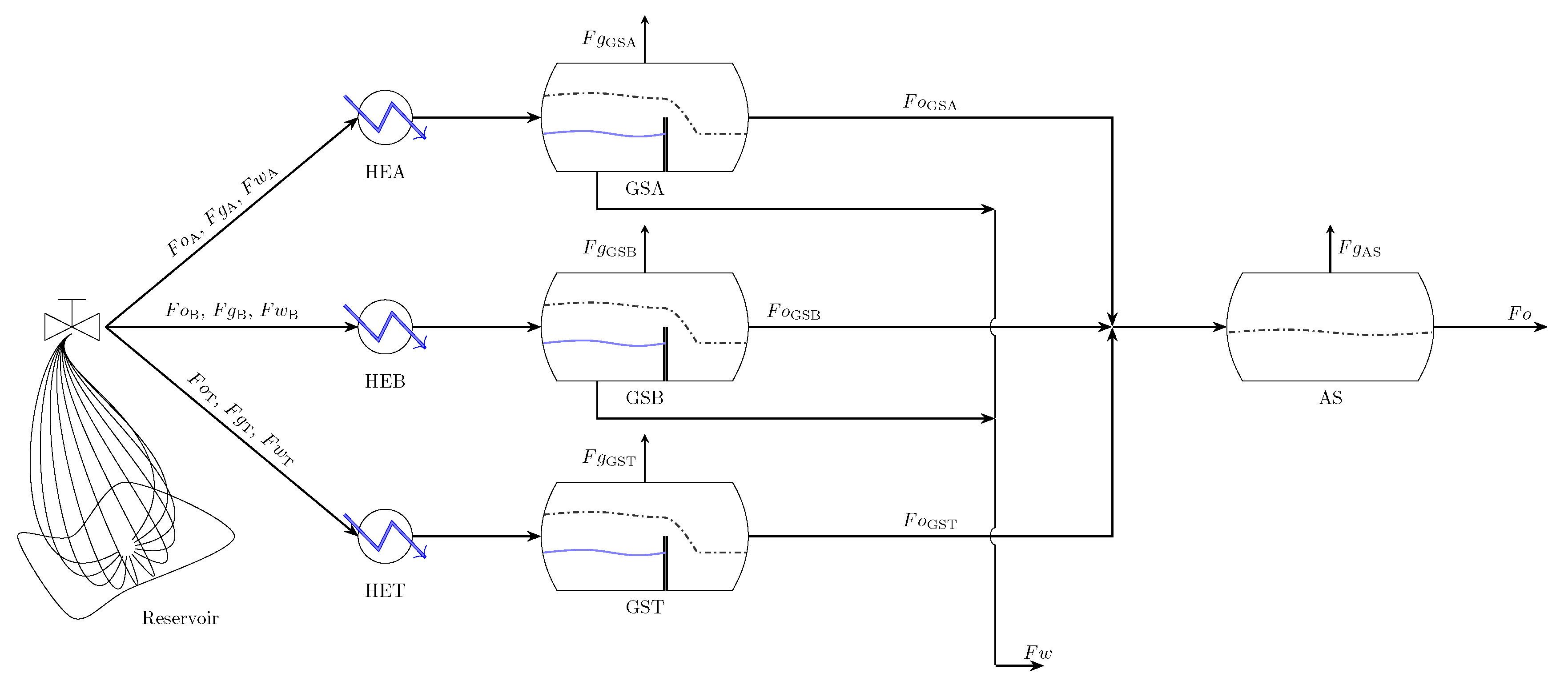
Figure 2.
Cumulative distribution function of the variability around the true values for each sample set.
Figure 2.
Cumulative distribution function of the variability around the true values for each sample set.
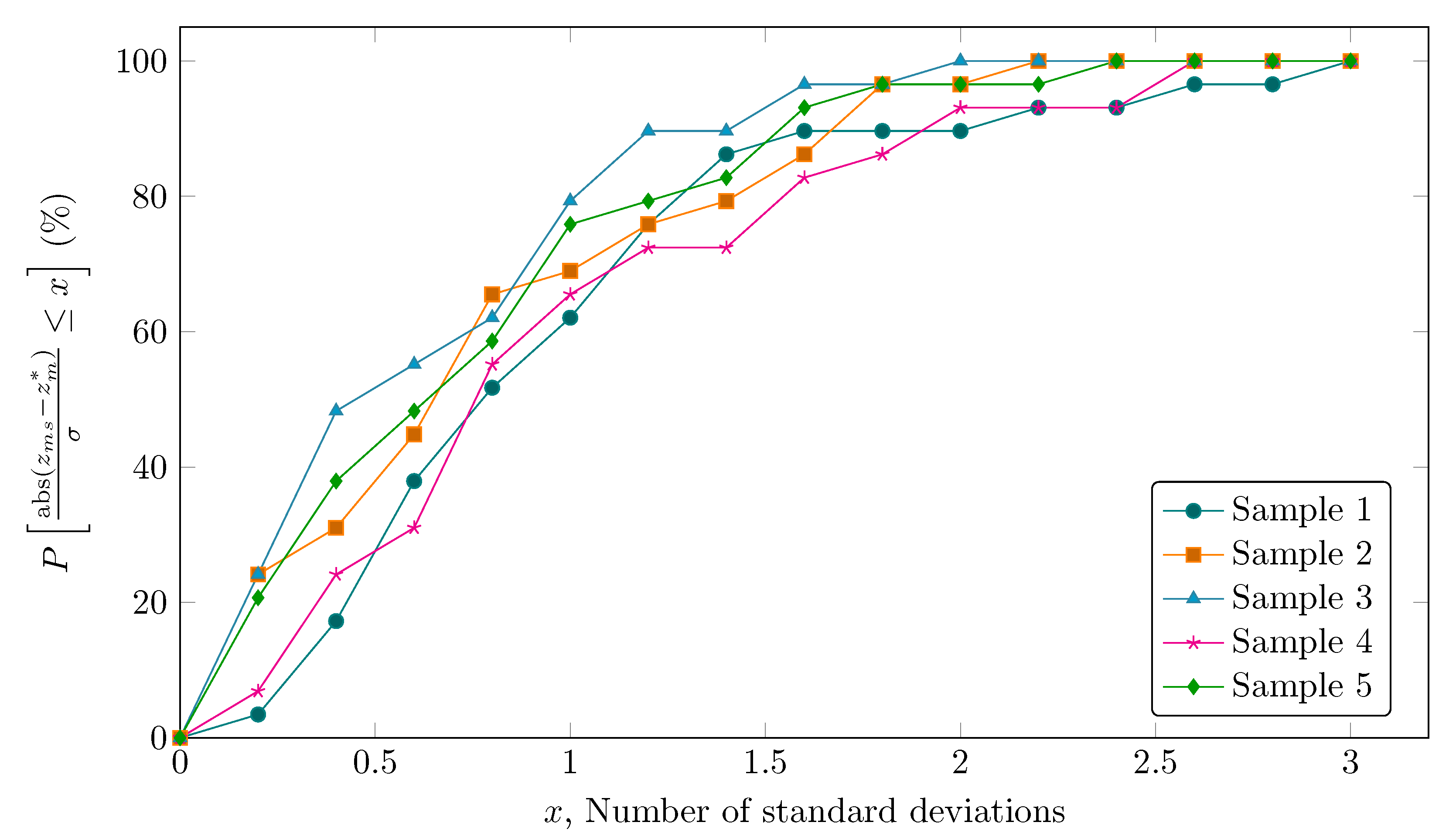
Figure 3.
Final objective function values after solving the DR problem as a function of the initial guess. (A) Forward finite difference; (B) Central finite difference.
Figure 3.
Final objective function values after solving the DR problem as a function of the initial guess. (A) Forward finite difference; (B) Central finite difference.
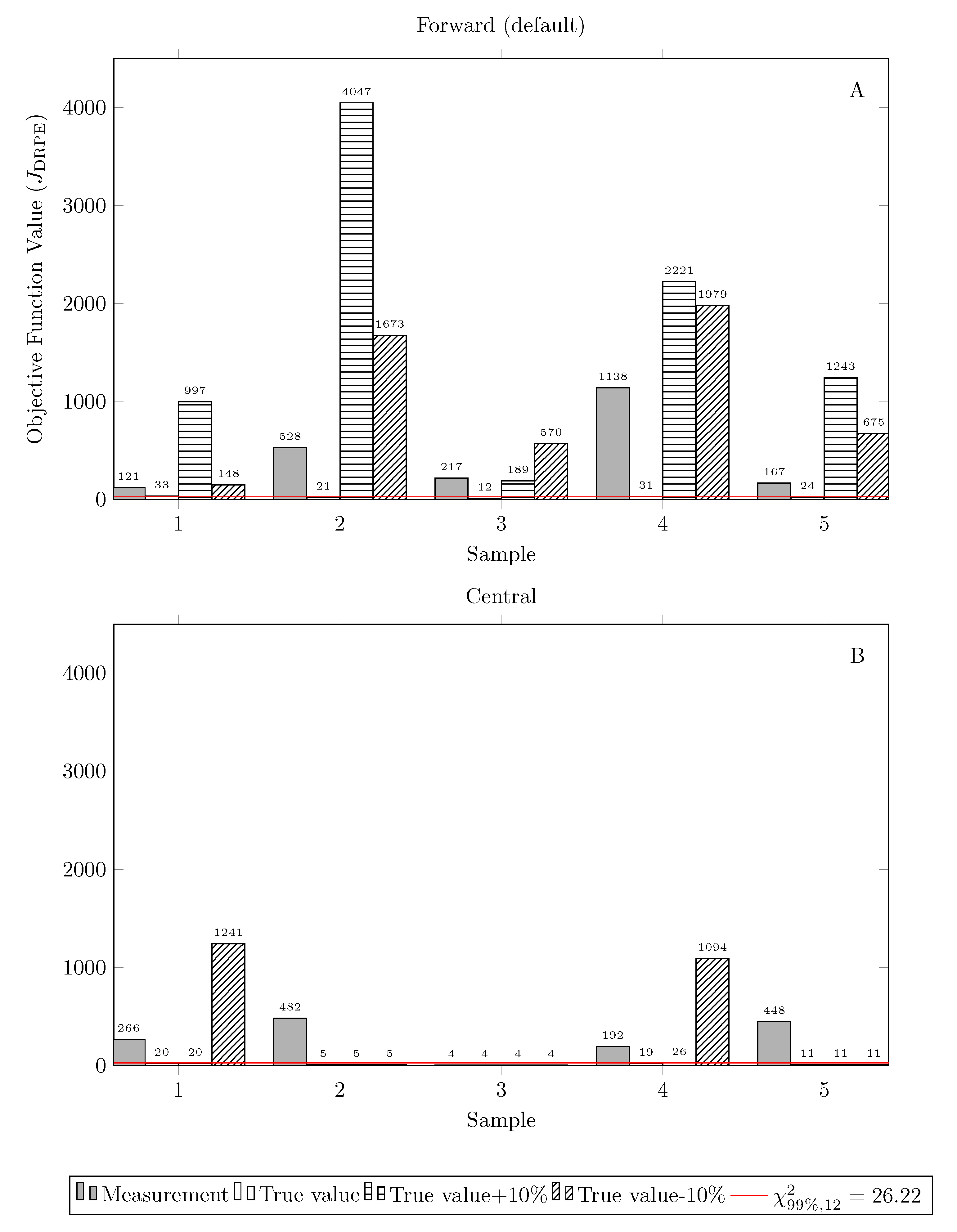
Figure 4.
Cumulative distribution function of the variability around the true values for each sample set for the DRPE results of settings 3 and 4.
Figure 4.
Cumulative distribution function of the variability around the true values for each sample set for the DRPE results of settings 3 and 4.
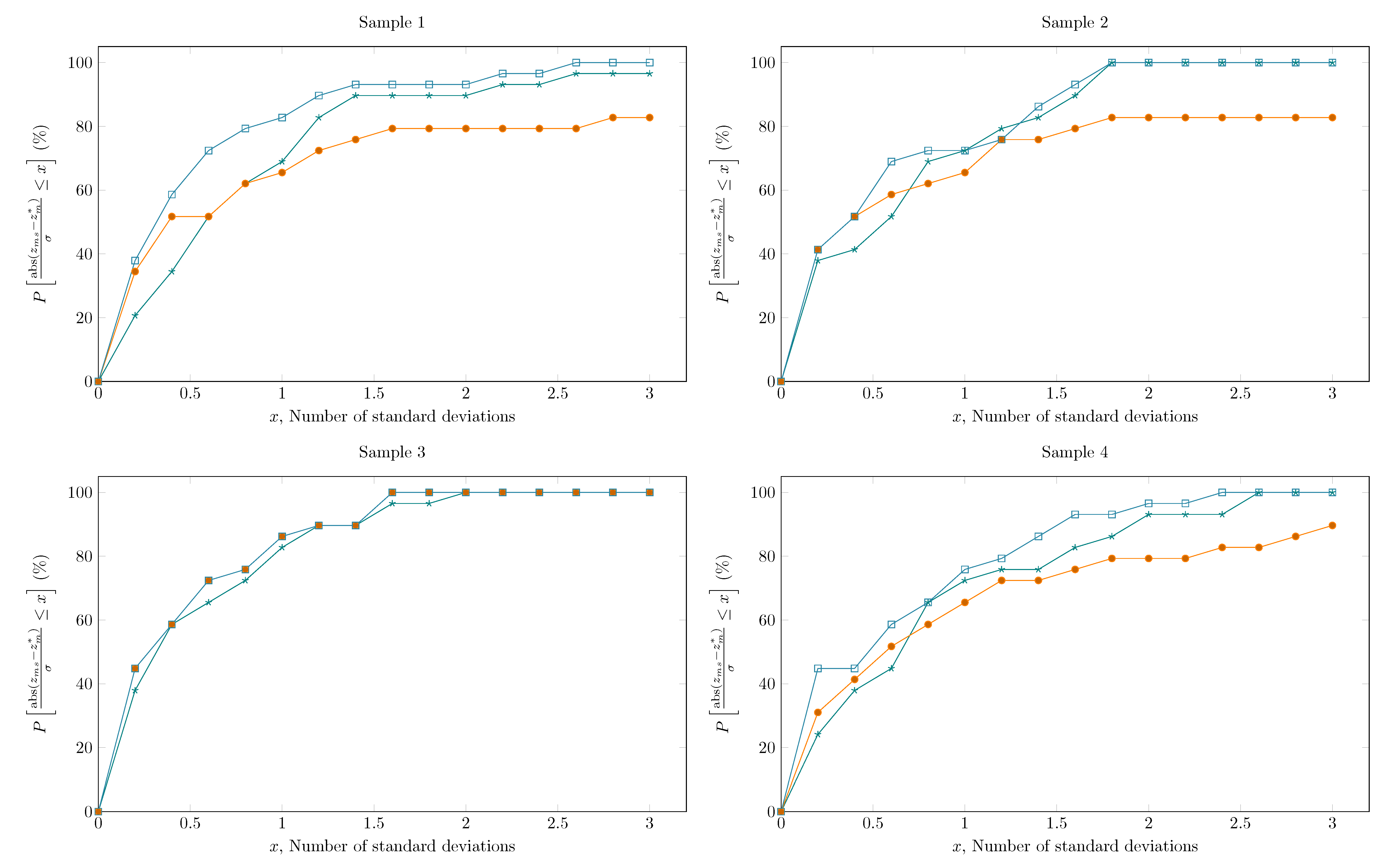

Figure 5.
Comparison of metrics for assessing reconciled results: (A) Relative difference between measured and reconciled data; (B) Normalized residue. DR results of setting 4.
Figure 5.
Comparison of metrics for assessing reconciled results: (A) Relative difference between measured and reconciled data; (B) Normalized residue. DR results of setting 4.
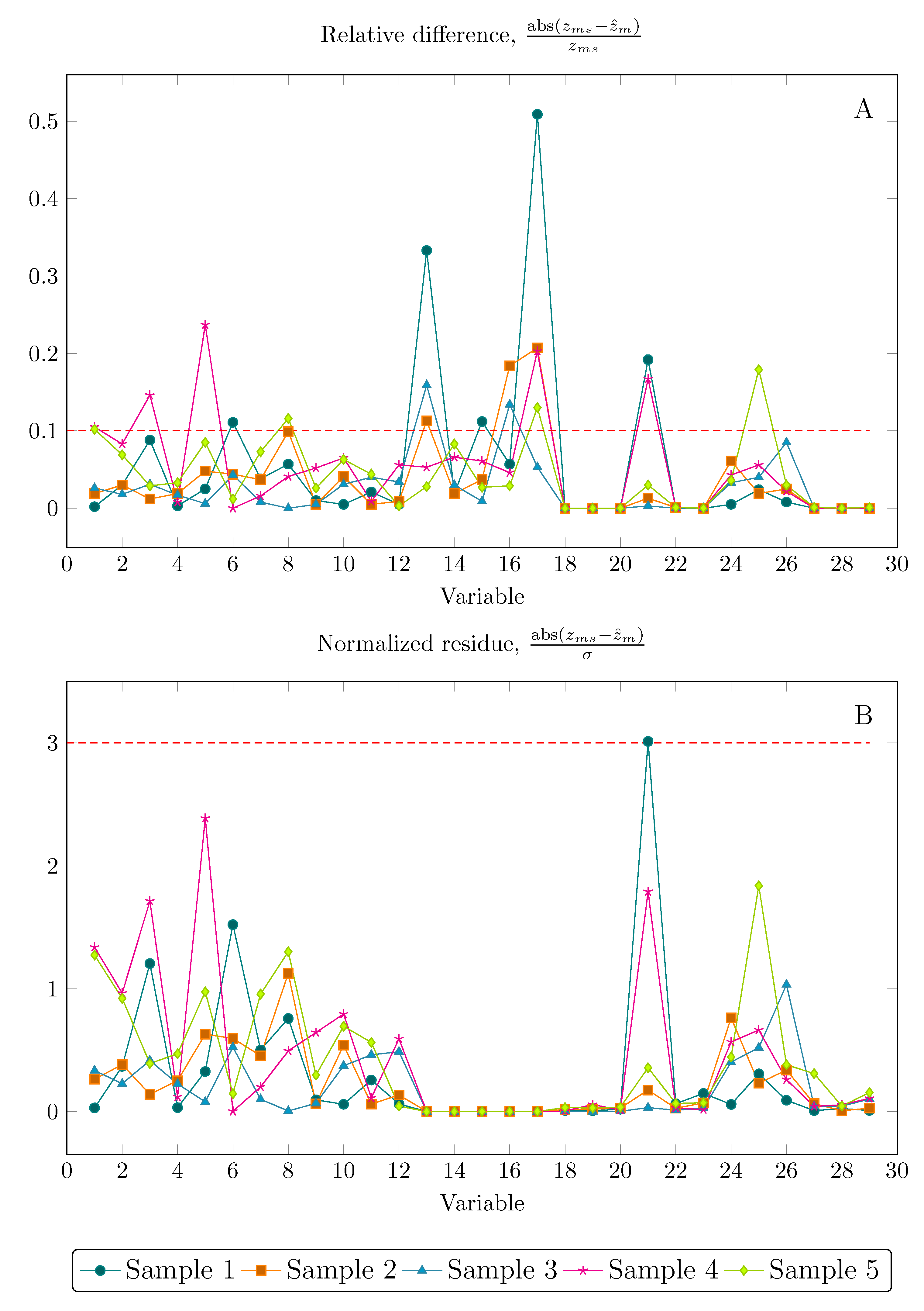

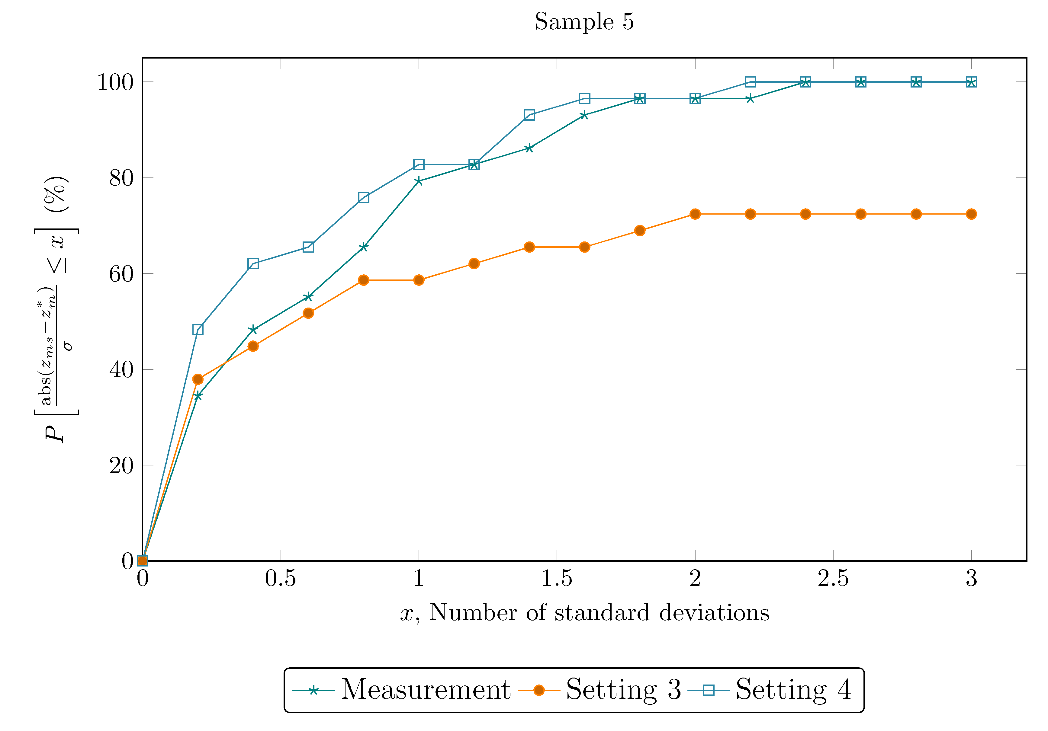
Table 1.
Real industrial applications of data reconciliation techniques or data reconciliation studies involving real plant data.
Table 1.
Real industrial applications of data reconciliation techniques or data reconciliation studies involving real plant data.
| Reference | Math. Nature | Estimator | Solution Method | Algorithm-Package/Simulator | Industrial Process |
|---|---|---|---|---|---|
| Hodouin and Everell [1] | static nonlinear | GL | Lagrange multipliers | Conjugate gradient method | Sections of mineral processing plant |
| Serth et al. [68] | static nonlinear | GL | Lagrange multipliers, Suc. Lin. | BSOLVE | Metallurgical grinding circuit |
| Holly et al. [69] | static linear | GL | Lagrange multipliers | analytical | Chemical extraction plant |
| Sanchez et al. [55] | static nonlinear | WLS | NLP solver | SQP/PLADAT | Ethylene plant |
| Meyer et al. [70] | static nonlinear | GL | Lagrange multipliers | Newton-Raphson | Beverage alcohol distillation plant |
| Islam et al. [58] | static nonlinear | GL | Linear solution, Suc. Lin., NLP solver | SQP | Industrial pyrolisis reactor |
| Krist et al. [60] | on-line static nonlinear | LS | Lagrange multipliers | Speedup/Aspenplus | Benzene plant |
| Bussani et al. [71] | on-line static nonlinear | WLS of relative errors | NLP solver | SQP/ORO | Hydrogen plant |
| Zhang et al. [10] | on-line static nonlinear | DR: contaminated gaussian, PE: LS | NLP solver | MINOS-GAMS/Aspen Plus | Monsanto sulfuric acid plant |
| Zhang et al. [72] | on-line static nonlinear | Contaminated gaussian | NLP solver | MINOS-GAMS/Aspen | Monsanto sulfuric acid plant |
| Weiss et al. [12] | static nonlinear | GL | Linear solution, Suc. Lin., NLP solver | Gauss-Marquardt, SQP | Industrial pyrolisis reactor |
| Sánchez et al. [73] | static nonlinear | GL | Linear solution, Suc. Lin., NLP solver | SQP | Industrial pyrolisis reactor |
| Sánchez and Romagnoli [74] | static (bi)linear | GL | Lagrange multipliers | Matrix Projection Method, QR decomposition | Industrial ethylene plant and simplified ammonia plant |
| Pierucci et al. [61] | on-line static nonlinear | WLS | NLP solver | SQP, Levenberg Marquardt, LNSI/ORO | Industrial furnace |
| Piccolo et al. [13] | static nonlinear | WLS | NLP solver | SQP/Apen Plus, MINOS5-GAMS | Refinery, gas separation system located downstream from a fluidized catalytic cracking unit |
| Heyen et al. [75] | static nonlinear | GL | Lagrange multipliers | NA | power plant |
| Kyriakopoulou and Kalitventzeff [53] | static nonlinear | GL | NLP solver | SQPIP, SOLDOG-BELSIM, SQPHP/VALI-BELSIM | Steam production network |
| Chiari et al. [50] | on-line static nonlinear | WLS of relative errors | NLP solver | SQP/ORO | Industrial hydrogen and sulfur plants |
| Christiansen et al. [76] | static nonlinear | GL | Suc. Lin., NLP solver | SQP | Industrial synthesis gas for production of ammonia |
| Heyen and Kalitventzeff [77] | static nonlinear | GL | NLP, MINLP | SQPIP, MINLP | Energy supply and utility distribution networks |
| McBrayer et al. [15] | dynamic nonlinear | WLS | NLP solver | SQP | Exxon chemical process |
| Dempf and List [78] | on-line static nonlinear | GL | NA | NA/VALI | Vinyl acetate and ketene plants |
| Plácido and Loureiro [79] | static nonlinear | GL | Lagrange multipliers | Matrix Projection Method | Ammonia plant |
| Bourouis et al. [80] | static nonlinear | Contaminated gaussian | NLP solver | NA | Multistage flash desalination plant |
| Chen et al. [51] | on-line static nonlinear | Contaminated gaussian, Lorentzian (GED-DR),WLS (DRPE) | NLP solver | CONOPT-GAMS | Sulfuric acid plant |
| Lee et al. [81] | on-line static (non)linear | GL | NLP solver | SQP | Industrial utility plant |
| Bazin et al. [82] | static nonlinear | GL | NLP solver | Conjugate gradient method | Rotary drier |
| Soderstrom et al. [83] | dynamic nonlinear | WLS | NLP solver | SQP-NOVA | Exxon chemical process |
| Li et al. [84] | on-line static nonlinear | WLS | Suc. Lin. | NA | Industrial crude oil distillation unit |
| Zhang et al. [85] | static linear | GL | Lagrange multipliers | NA | Refinery |
| Eksteen et al. [86] | static bilinear | 1. GL, 2. Closure residual | 1. NLP solver, 2. Lagrange multipliers | 1. GRG, 2. NA | Furnace from a pyrometallurgical industry |
| Sunde and Öivind Berg [87] | static nonlinear | GL | NA | NA/TEMPO system | Turbine cycle of a boiling water reactor (3300 MW) |
| Bagajewicz and Cabrera [88] | static nonlinear | GL | NLP solver | GAMS/SIMSCI | Gas pipeline systems |
| Vieira et al. [89] | dynamic nonlinear | GL | Lagrange multipliers | Gauss-Newton | Industrial polymerization reactor |
| Bhat and Saraf [56] | static linear | GL | Lagrange multipliers | analytical | Crude distillation unit |
| Chatterjee and Saraf [90] | static nonlinear | LS | NLP solver | SQP-NPSOL | Crude distillation unit refineries |
| Özyurt and Pike [28] | static nonlinear | Contaminated normal, Cauchy, Fair, Hampel, Logistic, and Lorentzian | NLP solver | Conopt2, Minos5 | Sulfuric acid plant |
| Yi and Han [91] | static MILP | GL | MILP | MILP | Gases network in an iron and steel making plant |
| Chen and Andersen [92] | static nonlinear | GL on closure residual | Lagrange multipliers | NA | Gas turbine |
| de Andrade Lima [93] | static nonlinear | GL | NLP solver | SQP-NPSOL | Industrial hydrometallurgical plants for gold extraction |
| AI-Arfaj [94] | static linear | GL | Lagrange multipliers | QR approach | Methyl-terc-butyl-ether plant |
| Faber et al. [95] | on-line static linear and nonlinear | Robust estimator of [96], Fair function | NLP solver | SQP - IMSL | Coke-oven-gas purification pilot plant |
| Hu and Shao [59] | static nonlinear | GL | Lagrange multipliers, Suc. Lin. | NA | Industrial coking plant |
| Prata et al. [47] | dynamic nonlinear | GL | NLP solver | Gauss-Newton | Industrial polymerization reactor |
| Faber et al. [23] | on-line static linear and nonlinear | Robust estimator of [96], Fair function | NLP solver | SQP - IMSL | Coke-oven-gas purification pilot plant |
| Schladt and Hu [97] | static nonlinear | Contaminated normal | NLP solver | SQP-SNOPT | Industrial distillation column |
| Bellec et al. [98] | online static bilinear | WLS | Kalman filter | Sigmafine (OSIsoft) | Paper machine stock approach system at an integrated newsprint paper mill |
| Lid and Skogestad [99] | static nonlinear | Contaminated normal | NLP solver | Fmincon-MATLAB | Refinery naphtha reformer |
| Reimers et al. [52] | static linear | GL | Lagrange multipliers | Gauss-Jordan/SolidSim | Dressing of brown coal |
| Embiruçu et al. [100] | dynamic nonlinear | GL | Lagrange multipliers | Gauss-Newton | Ethylene polymerization |
| Prata et al. [101] | dynamic nonlinear | GL | Lagrange multipliers | Gauss-Newton | Industrial polymerization reactor |
| Puig et al. [102] | static linear | GL | NA | Macrobal | Wastewater treatment plants (WWTPs) |
| Prata et al. [64] | dynamic nonlinear | GL | 1. Lagrange multipliers, 2. NLP solver | 1. Gauss-Newton, 2. PSO | Industrial polymerization reactor |
| Prata et al. [18] | dynamic nonlinear | GL, Welsch estimator | NLP solver | PSO | Industrial polypropylene reactor |
| Sarabia et al. [54] | on-line static nonlinear | GL | NLP solver | SQP-NAG/EcosimPro, IPOPT-GAMS | Hydrogen networks in oil refinery Petronor |
| Quelhas et al. [66] | on-line static nonlinear | GL | NLP solver | Gauss-Newton | Ethylene production |
| Zhang et al. [30] | static nonlinear | GL, Correntropy estimator | NA | NA | Air separation process |
| Cicciotti et al. [103] | static nonlinear | GL | NLP solver | NA | Multi-stage centrifugal compressor |
| Jiang et al. [104] | on-line static nonlinear | GL | Suc. Lin. | NA | Coal-fired steam turbine power plant (1000 MW) |
| Eghbal Ahmadi [105] | static nonlinear | GL | NLP solver | SQP/Aspen HySys | Part of a sulfur recovery unit |
| Guo et al. [106] | static nonlinear | GL | NLP solver | NA-MATLAB | Coal-fired steam turbine power plant (1000 MW) |
| Guo et al. [107] | static nonlinear | GL | NLP solver | SQP-fmincon/MATLAB | Coal-fired steam turbine power plant (1000 MW) |
| Behnami et al. [108] | static linear | WLS | Lagrange multipliers | MATLAB | Full-scale petrochemical wastewater treatment plant (WWTP) |
| Rafiee and Behrouzshad [109] | static nonlinear | GL | NLP solver | Fmincon-MATLAB | Natural gas processing plant |
| Câmara et al. [67] | on-line static nonlinear | WLS | NLP solver | SQP | Crude oil distillation |
WLS–Weighted least squares; GL–Gaussian likelihood (WLS); SQP–Successive quadratic programming; NLP–Nonlinear programming; NA–Not available.
Table 2.
Information regarding process model variables and parameters.
| Variable | Type | Unit | CV (%) |
|---|---|---|---|
| Inlet oil stream of HEA | 1 | m/day | 8 |
| Inlet gas stream of HEA | 1 | m/day | 8 |
| Inlet water stream of HEA | 1 | m/day | 8 |
| Inlet oil stream of HEB | 1 | m/day | 8 |
| Inlet gas stream of HEB | 1 | m/day | 8 |
| Inlet water stream of HEB | 1 | m/day | 8 |
| Inlet oil stream of HET | 1 | m/day | 8 |
| Inlet gas stream of HET | 1 | m/day | 8 |
| Inlet water stream of HET | 1 | m/day | 8 |
| Water feed stream of HEA | 1 | m/day | 8 |
| Water feed stream of HEB | 1 | m/day | 8 |
| Water feed stream of HET | 1 | m/day | 8 |
| Overall heat transfer coefficient of HEA | 2 | kcal m h C | 8 |
| Overall heat transfer coefficient of HEB | 2 | kcal m h C | 8 |
| Overall heat transfer coefficient of HET | 2 | kcal m h C | 8 |
| Split coefficient of SGA | 2 | % | 8 |
| Split coefficient of SGB | 2 | % | 8 |
| Outlet gas stream of SGA | 3 | m/day | 0.2 |
| Outlet gas stream of SGB | 3 | m/day | 0.2 |
| Outlet gas stream of SGT | 3 | m/day | 0.2 |
| Outlet gas stream of AS | 3 | m/day | 8 |
| Discharged water stream | 3 | m/day | 2 |
| Exported oil stream | 3 | m/day | 0.2 |
| Temperature of outlet water stream of HEA | 3 | C | 8 |
| Temperature of outlet water stream of HEB | 3 | C | 8 |
| Temperature of outlet water stream of HET | 3 | C | 8 |
| Temperature of outlet oil stream of HEA | 3 | C | 0.4 |
| Temperature of outlet oil stream of HEB | 3 | C | 0.4 |
| Temperature of outlet oil stream of HET | 3 | C | 0.4 |
Table 3.
Configuration settings of simulation experiments.
| Setting | Solution Approach | Finite Difference | Initial guess | Degrees of Freedom | Optimization Algorithm | |
|---|---|---|---|---|---|---|
| 1 | simultaneous | central | measurement | yes | 12 | IP |
| 2a | sequential | central | measurement | yes | 12 | IP |
| 2b | sequential | central | true value | yes | 12 | IP |
| 2c | sequential | central | true value + 10% | yes | 12 | IP |
| 2d | sequential | central | true value − 10% | yes | 12 | IP |
| 2e | sequential | forward | measurement | yes | 12 | IP |
| 2f | sequential | forward | true value | yes | 12 | IP |
| 2g | sequential | forward | true value + 10% | yes | 12 | IP |
| 2h | sequential | forward | true value − 10% | yes | 12 | IP |
| 3 | sequential | central | measurement | no | 7 | IP |
| 4 | sequential | central | measurement | no | 7 | PSO/IP |
Table 4.
Non-default values of optimization options used in fmincon routine in DR runs.
| Parameter | Description | Value |
|---|---|---|
| TolFun | Termination tolerance on the function value | 1 × 10 |
| TolX | Termination tolerance on decision variables | 1 × 10 |
| MaxIter | Maximum number of iterations allowed | 5000 |
| MaxFunEvals | Maximum number of function evaluations allowed | 10,000 |
Table 5.
Parameter values of PSO algorithm.
| Description | Value |
|---|---|
| Number of generations | 60 |
| Number of particles | 5 |
| Local search parameter | 1 |
| Global search parameter | 1 |
Table 6.
Objective function values and computational cost as a function of solution approach.
| Sample | Time (min) | |||||
|---|---|---|---|---|---|---|
| Simultaneous (Setting 1) | Sequential (Setting 2a) | Relative Difference (%) | Simultaneous (Setting 1) | Sequential (Setting 2a) | Relative Difference (%) | |
| 1 | 347 | 266 | −23 | 54 | 9 | −83 |
| 2 | * 633 | 482 | −24 | 14 | 9 | −34 |
| 3 | * 62 | 4 | −93 | 63 | 29 | −54 |
| 4 | * 3352 | 192 | −94 | 77 | 8 | −89 |
| 5 | 990 | 448 | −55 | 50 | 9 | −81 |
* No feasible point was found, as indicated by the value of output variable exitflag of fmincon routine.
Table 7.
Final objective function values after solving the DR problem as a function of the initial guess and type of finite difference.
Table 7.
Final objective function values after solving the DR problem as a function of the initial guess and type of finite difference.
| Setting | 2e | 2a | 2f | 2b | 2g | 2c | 2h | 2d |
|---|---|---|---|---|---|---|---|---|
| Initial Guess | Measurement | True Value | (True Value) × 1.1 | (True Value) × 0.9 | ||||
| Sample\Finite Difference | Forward | Central | Forward | Central | Forward | Central | Forward | Central |
| 1 | 121 | 266 | 33 | 20 | 997 | 20 | 148 | 1241 |
| 2 | 528 | 482 | 21 | 5 | 4047 | 5 | 1673 | 5 |
| 3 | 217 | 4 | 12 | 4 | 189 | 4 | 570 | 4 |
| 4 | 1138 | 192 | 31 | 19 | 2221 | 26 | 1979 | 1094 |
| 5 | 167 | 448 | 24 | 11 | 1243 | 11 | 675 | 11 |
| Average | 434 | 279 | 24 | 12 | 1739 | 13 | 1009 | 471 |
| Relative difference (%) | −36 | −50 | −99 | −53 | ||||
Table 8.
Elapsed time (min) for solving the DR problem as a function of the initial guess and type of finite difference.
Table 8.
Elapsed time (min) for solving the DR problem as a function of the initial guess and type of finite difference.
| Setting | 2e | 2a | 2f | 2b | 2g | 2c | 2h | 2d |
|---|---|---|---|---|---|---|---|---|
| Initial Guess | Measurement | True Value | (True Value) × 1.1 | (True Value) × 0.9 | ||||
| Sample\Finite Difference | Forward | Central | Forward | Central | Forward | Central | Forward | Central |
| 1 | 33 | 9 | 6 | 22 | 13 | 24 | 29 | 8 |
| 2 | 70 | 9 | 18 | 21 | 3 | 29 | 5 | 24 |
| 3 | 25 | 29 | 31 | 20 | 26 | 31 | 5 | 23 |
| 4 | 6 | 8 | 3 | 14 | 27 | 24 | 22 | 14 |
| 5 | 60 | 9 | 2 | 25 | 12 | 27 | 33 | 26 |
| Average | 39 | 13 | 12 | 21 | 16 | 27 | 19 | 19 |
| Relative difference (%) | −67 | 72 | 65 | 0 | ||||
Table 9.
Averaged results of objective function values and computational cost for different samples according to the type of finite difference.
Table 9.
Averaged results of objective function values and computational cost for different samples according to the type of finite difference.
| Sample | Time (min) | |||||
|---|---|---|---|---|---|---|
| Forward | Central | Relative Difference (%) | Forward | Central | Relative Difference (%) | |
| 1 | 325 | 387 | 19 | 20 | 16 | −22 |
| 2 | 1567 | 125 | −92 | 24 | 21 | −15 |
| 3 | 247 | 4 | −98 | 22 | 26 | 19 |
| 4 | 1342 | 333 | −75 | 14 | 15 | 6 |
| 5 | 527 | 120 | −77 | 27 | 22 | −18 |
Table 10.
Objective function values and computational cost as a function of problem formulation.
| Sample | Time (min) | |||||
|---|---|---|---|---|---|---|
| (Setting 2a) | (Setting 3) | Relative Difference (%) | (Setting 2a) | (Setting 3) | Relative Difference (%) | |
| 1 | 266 | 485 | 82 | 9 | 6 | −32 |
| 2 | 482 | 1042 | 116 | 9 | 4 | −52 |
| 3 | 4 | 3 | −38 | 29 | 24 | −17 |
| 4 | 192 | 171 | −11 | 8 | 9 | 8 |
| 5 | 448 | 528 | 18 | 9 | 5 | −41 |
Table 11.
Number of variables whose reconciled value is out of the confidence region of 99.7%.
| Sample | (Setting 2a) | (Setting 3) |
|---|---|---|
| 1 | 6 | 5 |
| 2 | 5 | 5 |
| 3 | 0 | 0 |
| 4 | 6 | 3 |
| 5 | 6 | 8 |
Table 12.
Objective function values and computational cost as a function of problem formulation.
| Sample | Time (min) | |||||
|---|---|---|---|---|---|---|
| IP (Setting 3) | PSO + IP (Setting 4) | Relative Difference (%) | IP (Setting 3) | PSO + IP (Setting 4) | Relative Difference (%) | |
| 1 | 485 | 748/14 | −97 | 6 | 7 + 21 = 28 | 354 |
| 2 | 1042 | 89/4 | −99.7 | 4 | 6 + 11 = 17 | 309 |
| 3 | 3 | 578/3 | 0 | 24 | 6 + 22 = 28 | 16 |
| 4 | 171 | 291/17 | −90 | 9 | 6 + 11 = 17 | 91 |
| 5 | 528 | 686/11 | −98 | 5 | 6 + 13 = 19 | 242 |
© 2017 by the authors. Licensee MDPI, Basel, Switzerland. This article is an open access article distributed under the terms and conditions of the Creative Commons Attribution (CC BY) license (http://creativecommons.org/licenses/by/4.0/).
Share and Cite
MDPI and ACS Style
Câmara, M.M.; Soares, R.M.; Feital, T.; Anzai, T.K.; Diehl, F.C.; Thompson, P.H.; Pinto, J.C. Numerical Aspects of Data Reconciliation in Industrial Applications. Processes 2017, 5, 56. https://doi.org/10.3390/pr5040056
AMA Style
Câmara MM, Soares RM, Feital T, Anzai TK, Diehl FC, Thompson PH, Pinto JC. Numerical Aspects of Data Reconciliation in Industrial Applications. Processes. 2017; 5(4):56. https://doi.org/10.3390/pr5040056
Chicago/Turabian StyleCâmara, Maurício M., Rafael M. Soares, Thiago Feital, Thiago K. Anzai, Fabio C. Diehl, Pedro H. Thompson, and José Carlos Pinto. 2017. "Numerical Aspects of Data Reconciliation in Industrial Applications" Processes 5, no. 4: 56. https://doi.org/10.3390/pr5040056
Note that from the first issue of 2016, this journal uses article numbers instead of page numbers. See further details here.