Article

Multistage Stochastic Programming Models for Pharmaceutical Clinical Trial Planning

Department of Chemical Engineering, Auburn University, Auburn, AL 36849, USA
*
Author to whom correspondence should be addressed.
Processes 2017, 5(4), 71; https://doi.org/10.3390/pr5040071
Submission received: 19 September 2017 / Revised: 20 October 2017 / Accepted: 25 October 2017 / Published: 9 November 2017

Abstract

:
Clinical trial planning of candidate drugs is an important task for pharmaceutical companies. In this paper, we propose two new multistage stochastic programming formulations (CM1 and CM2) to determine the optimal clinical trial plan under uncertainty. Decisions of a clinical trial plan include which clinical trials to start and their start times. Its objective is to maximize expected net present value of the entire clinical trial plan. Outcome of a clinical trial is uncertain, i.e., whether a potential drug successfully completes a clinical trial is not known until the clinical trial is completed. This uncertainty is modeled using an endogenous uncertain parameter in CM1 and CM2. The main difference between CM1 and CM2 is an additional binary variable, which tracks both start and end time points of clinical trials in CM2. We compare the sizes and solution times of CM1 and CM2 with each other and with a previously developed formulation (CM3) using different instances of clinical trial planning problem. The results reveal that the solution times of CM1 and CM2 are similar to each other and are up to two orders of magnitude shorter compared to CM3 for all instances considered. In general, the root relaxation problems of CM1 and CM2 took shorter to solve, CM1 and CM2 yielded tight initial gaps, and the solver required fewer branches for convergence to the optimum for CM1 and CM2.

1. Introduction

Pharmaceutical industry is a global business with over one trillion U.S. dollars per year market with extensive supply chains throughout the world [1]. A potential drug identified at discovery stage has to go through pre-clinical testing, generally laboratory and animal model studies, before applying for approval by regulatory bodies, such as The Food and Drug Administration (FDA) in USA. The goal of these laboratory and animal model studies is to understand how the drug works and assess its safety. The potential drugs that successfully complete pre-clinical trials enter clinical trial phase. Clinical trials aim to demonstrate the safety and efficacy of the potential drug and are designed with and carried out under strict guidelines and supervision of regulatory bodies. If a drug successfully completes the clinical trials and is approved by the regulatory bodies, the drug is manufactured and distributed to the market. Pharmaceutical manufacturers are under pressure to improve the efficiency of the pharmaceutical R&D pipeline, partially because the patent protections of a number of significant brand-name drugs will soon expire [2].
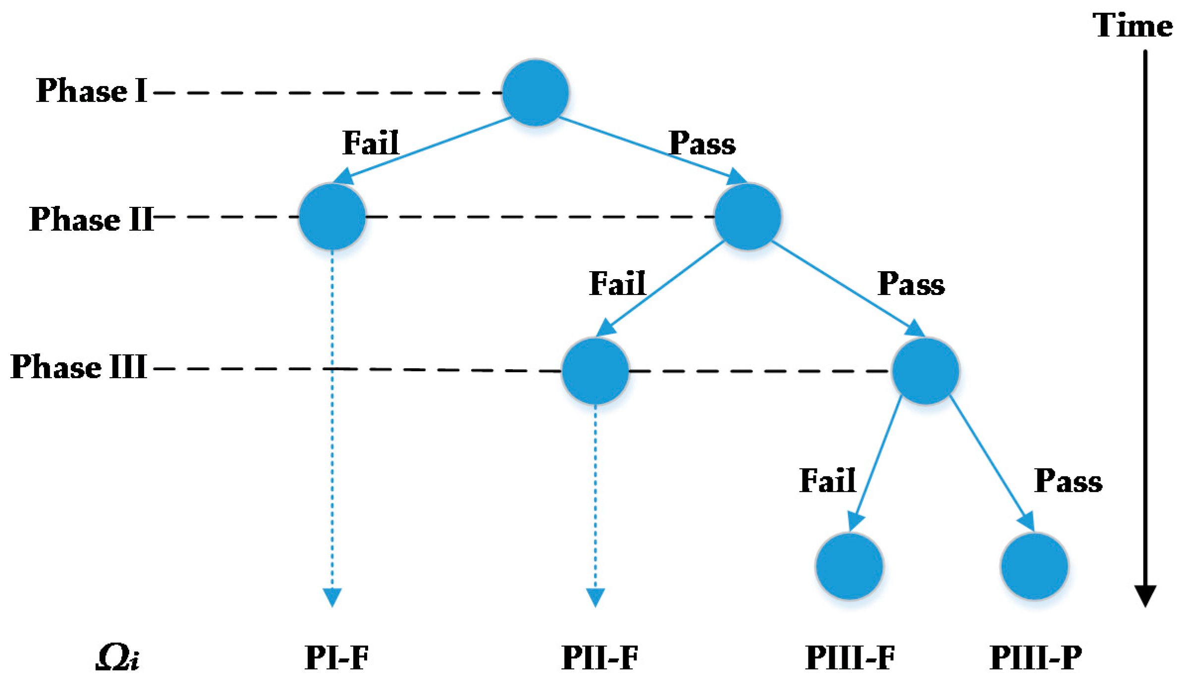
Scheduling and planning of clinical trials is one of the efficient ways to reduce the cost of developing new drugs. There are three phases in clinical trials. The goal of Phase I clinical trials is to assess the safety and dosage of the drug and to understand how it is metabolized in the body. The lengths of Phase I clinical trials are several months. Approximately 70% of drugs will move to the next phase. Phase II clinical trials are used to evaluate the drug’s effectiveness and short-term side effects on a limited number of target patient volunteers. Phase II may take from several months to two years. Approximately 33% of drugs pass Phase II clinical trials and move to the next stage. Phase III clinical trials aim to assess the benefit-risk ratio of the drug using a large number of target patient volunteers (in the order of thousands). Phase III takes one to four years to complete and approximately 25–30% of drugs pass Phase III [3,4]. Clinical trial planning is complicated due to its highly stochastic nature: pharmaceutical companies do not know which drugs will successfully complete clinical trials a priori. The outcomes of clinical trials significantly influence drug development plan, the investments and overall profits. Clinical trial planning is a series of trade-offs between maximizing expected economic returns and minimizing risk and maintaining a diverse portfolio of drugs under the limited drug development dollars available. The plan tries to accomplish these goals by selecting which potential drugs to push through the clinical trial pipeline and when to start the clinical trials of selected drugs. This is a challenging problem due to its strong combinatorial character and impact of uncertainty.
Stochastic programming is a framework for modeling optimization problems that involve uncertainty [
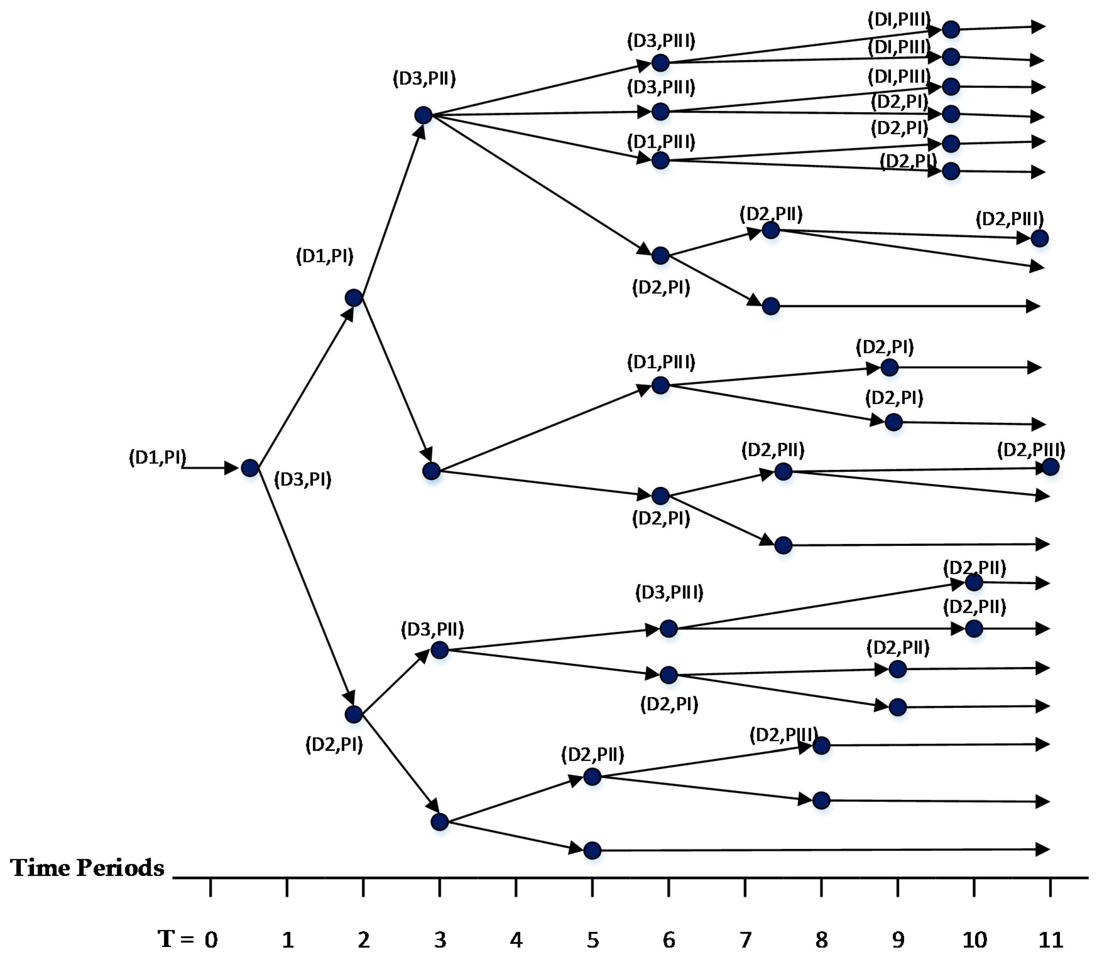
5]. Stochastic programming optimizes the expected value of the decisions over all possible realizations of uncertain parameters. A set of scenarios describes all possible realizations of uncertain parameters. In clinical trial planning problem, the uncertain parameter is the outcome of a clinical trial and it is an endogenous uncertain parameter because the decisions of whether or not and when to start clinical trials influence when the outcomes are realized. We assume that there are two discrete outcomes of a drug starting and completing a clinical trial: (1) the drug may successfully pass the clinical trial; or (2) the drug may fail the clinical trial. Because the outcomes are discrete, all combinations of possible realizations can be used to form a finite set of scenarios for the clinical trial planning problem. To consider recourse action in multiple stages after realizations of uncertainty, one of the widely used approaches employs multistage stochastic programming (MSSP). To avoid making decisions that anticipate the values of uncertain parameters that have not been realized, a set of constraints, called non-anticipativity constraints (NACs), are introduced to MSSPs.
Multistage stochastic programming is a scenario-based approach that considers recourse actions in multiple stages after realization of uncertainty. In the MSSP formulations of problems with endogenous uncertainty, decision variables are defined independently for each scenario. For formulations whose objective function and constraints are all linear and include integer variables, the deterministic equivalent of the MSSP can be constructed as a mixed-integer linear programming (MILP) model.
The general formulation of a MSSP with endogenous uncertainty can be written as follows:
min s p s f ( x l , t s , γ t s )
g k , t ( x l , t s , γ t s ) 0           k , s , t
x l , 1 s = x l , 1 s                   s , s
[ y t s , s x l , t s = x l , t s γ t s = γ t s ] [ ¬ y t s , s ]               s , s , t > 1
y t s , s   H ( x l , 1 s , x l , 2 s , , x l , t s )             s , s ,   t
y t s { 0 , 1 }           γ t s   ,   x l , t s
where f , g k , t are differentiable functions, k is the index for the set of scenario-specific constraints, t is the index for the set of discrete time periods, s is the index of the set of scenarios and p s is the probability of scenario s . The variable x l , t s is the decision variable associated with endogenous uncertain parameter l at time t in scenario s . The variable γ t s is recourse-action variable at time t ( t > 1 ) in scenario s . The objective is to minimize the expected value of f . Functions g k , t define the scenario-specific constraints. At the first time period, the values of decision variables must be identical because all scenarios are indistinguishable (Equation (3)). The variable y t s , s is a Boolean variable, which indicates when scenarios s and s’ are indistinguishable. If y t s , s is True, then the decision variables and recourse actions for these scenarios should be identical (Equation (4)). The value of the Boolean variable depends on the decision variable values, as shown in Equation (5). If functions f , g k , t are all linear, the deterministic equivalent of MSSP can be formulated as a MILP model.
There have been a number of studies that introduced stochastic programing models for solving pharmaceutical clinical trial planning problem. Here, we limit our review to the ones that explicitly incorporated the impact of clinical trial outcome uncertainty. Gatica et al. [6] developed a model that integrates the production planning and investment strategy simultaneously in pharmaceutical industries considering the impact of uncertainty in the outcome of clinical trials. The case studies considered in the paper included only two phases of the clinical trials with three products yielding 64 scenarios. However, if all stages of clinical trials were considered, the size of the resulting model would have become prohibitively large and would require heuristic approaches to solve. Colvin and Maravelias [7] developed a MSSP model for clinical trial planning and included the impact of endogenous clinical-trial outcome uncertainty. In a later study, they exploited the structure of the problem to reduce the number of scenarios and extended their model to account for resource planning by introducing outsourcing decisions [8]. In Reference [9], they introduced a number of theoretical properties, which reduce the problem size and tighten the formulation, and developed a novel branch and cut algorithm to solve the resulting problem efficiently. Sundaramoorthy et al. [10] proposed a stochastic programming formulation that integrates the capacity planning and clinical trial planning and that takes into account uncertainty in the outcomes of clinical trials. The proposed formulation was solved for problems with a total of 256 scenarios in 1127 CPUs. The solution time increases significantly for problems with more than 256 scenarios.
Multistage stochastic programs and their deterministic equivalent forms quickly become computationally intractable because the number of scenarios and the corresponding decision trees grow exponentially as the number of uncertain parameters increases. Furthermore, for discrete-time MSSPs, the problem size increases rapidly especially in numbers of variables and NACs with increases in the length of the planning horizon. Thus, solving any large-scale MSSP model, especially with endogenous uncertainty, requires significant computational effort. Most recent work on MSSPs with endogenous uncertainty focuses on developing new algorithms or decomposition frameworks for solving these problems.
Solak et al. [11] developed a sample average approximation (SAA) algorithm to solve the optimization problem of R&D project portfolio. The proposed algorithm approximates the MSSP formulation with smaller MSSPs constructed using a random sample of scenarios selected from the full set. For the case studies considered, the SAA algorithm obtained a solution within 3.4–8.3% of the optimal. Gupta and Grossmann [12] proposed an improved lagrangean decomposition framework, which decomposed the original problem into individual scenario groups. For process synthesis and oilfield planning problems, the improved lagrangean decomposition framework obtained tighter bounds with fewer iterations. Christian and Cremaschi [13] developed a knapsack-problem based decomposition algorithm (KDA) for solving pharmaceutical clinical trial planning problem. The KDA obtains feasible solutions by decomposing the original MSSP problem into a series of knapsack problems. Instead of characterizing all realizations as scenarios, the KDA generates knapsack problems at time periods when outcomes are realized. Solutions obtained by KDA were within three percent of the optimum for the case studies considered. Christian and Cremaschi [14] presented a branch and bound algorithm to solve large-scale MSSPs with endogenous uncertainty. The algorithm generates dual bounds using progressive hedging (PH) and primal bounds using the KDA [14]. Although the algorithm required considerable time to converge, it reduced the memory requirements considerably. Apap and Grossmann [15] proposed a sequential scenario decomposition (SSD) approach for solving MSSPs with endogenous and exogenous uncertainties. The algorithm starts at the initial time period and selects one scenario from each exogenous scenario group. A sub-problem is constructed by removing all NACs associated with the exogenous uncertain parameters. The scenarios in the sub-problem are only connected by first-time period NACs and NACs associated with the endogenous uncertain parameter. The solution of the sub-problem is used to fix the variables of the original MSSP at first-time period. The algorithm repeats this process until the end of the planning horizon. At termination, all decisions are fixed in original MSSPs yielding a feasible solution. For the oilfield development planning problem [15], the SSD solution was within 0.2% of the optimum.
Most of these algorithms decompose the original problem into smaller sub-problems to generate a feasible solution. No recent literature studied the impact of different decision variable definitions and corresponding sequencing and non-anticipativity constraints on the size and solution times of the resulting MSSP formulations constructed for clinical trial planning.
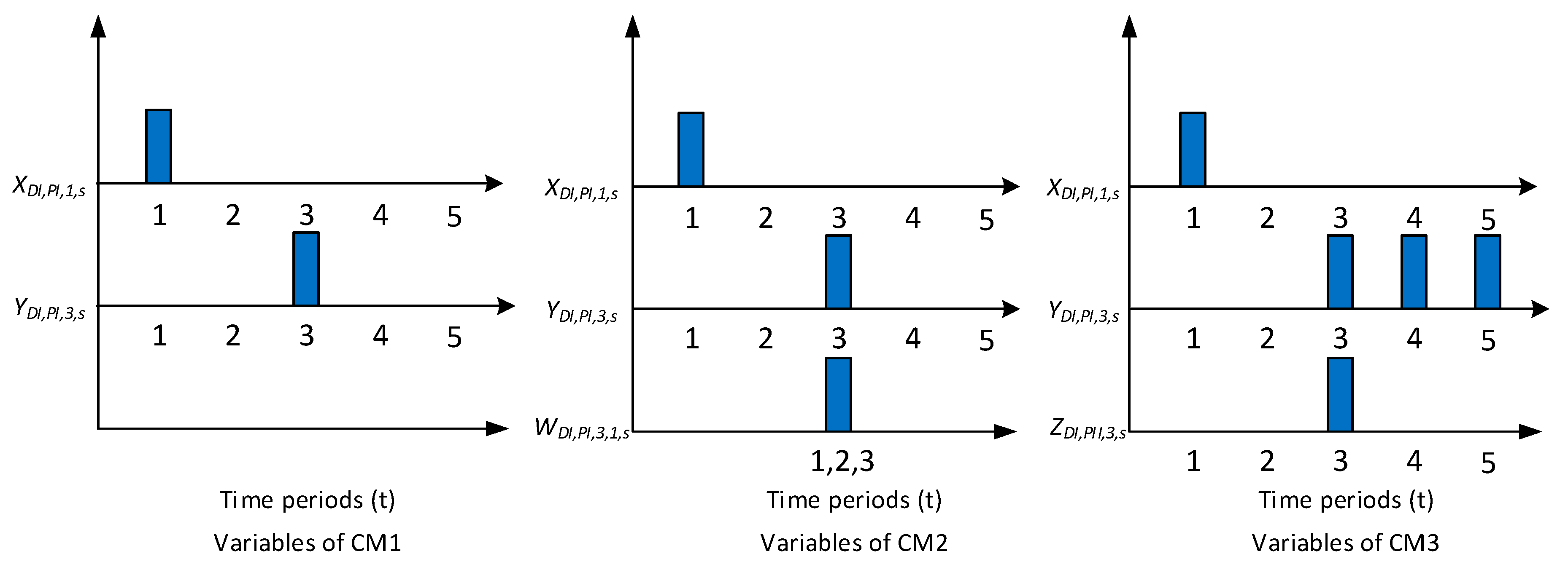
Motivated by the above, we propose two new MSSP formulations, CM1 and CM2, for pharmaceutical clinical trial planning problem. The first formulation, CM1, employs two decision variables, which separately track the start and end time points of clinical trials. The second formulation, CM2, introduces an additional binary variable, which tracks both start and end time points of a clinical trial. We applied both formulations to solve 42 instances of clinical trial planning problem [16]. For comparison, all instances were also solved using the MSSP formulation of [
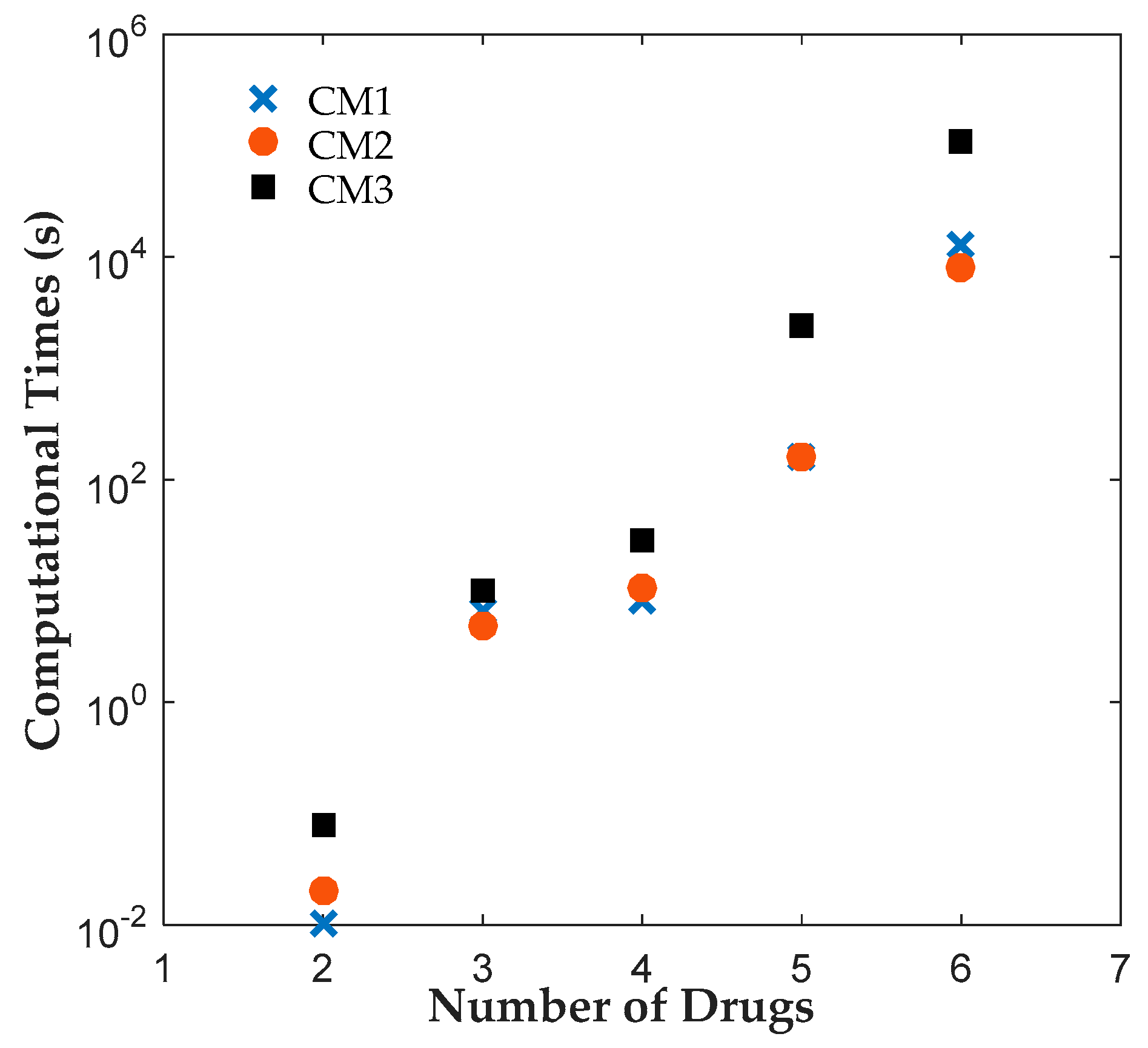
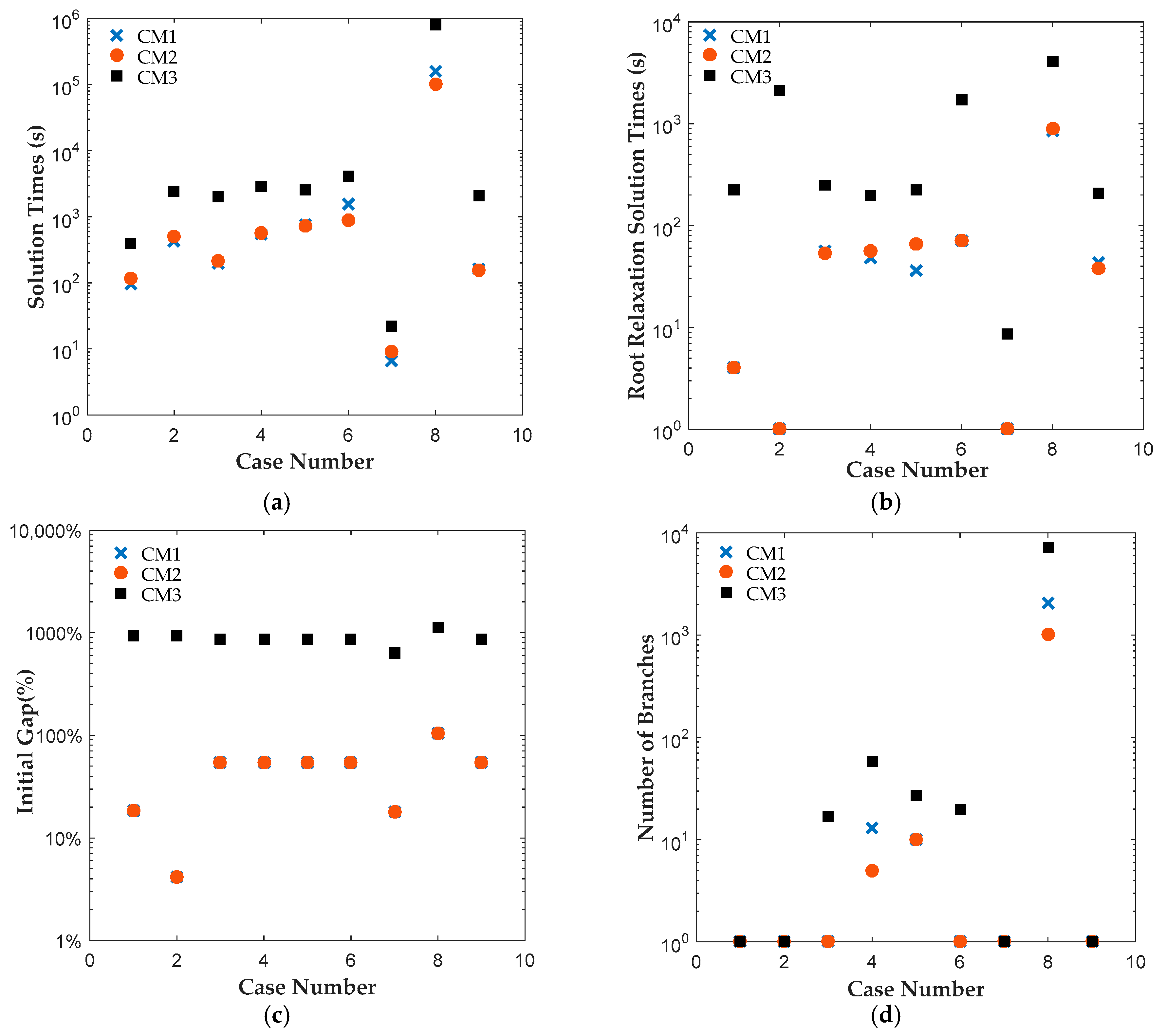
7], which will be referred to as CM3 here. All instances were solved to 0.1% optimality gap using ILOG CPLEX Optimization Studio (Version 12.6.3.0, IBM, Armonk, NY, USA). The results reveal that CM1 and CM2 were consistently solved up to two orders of magnitude faster than CM3 for all cases. A closer look at the branching trees indicates that the optimum was obtained with fewer branches for CM1 or CM2 than CM3. Section 2 gives the clinical trial planning problem statement. New MSSP formulations are presented in Section 3. Section 4 summarizes and discusses the results of the computational studies. Conclusion are summarized in Section 5.

2. Problem Statement

Following the problem definition of [7] and nomenclature given in Appendix A, the problem addressed in this paper can be stated as follows. Givens are
(1)
A set of candidate drugs ( i I ) that should go through a set of clinical trials ( j J = { P I ,   P I I ,   P I I I } ) ,
(2)
The length of the planning horizon, which is discretized into equal time periods p   =   1 ,   2 ,   3 T (period p starts at time p 1 and ends at time p ), t   =   1 ,   2 ,   3 T + m a x i j ( τ i j   i I , j J ) (period t starts at time t 1 and ends at time t ),
(3)
Cost C i j , resource requirements(s) ρ i j r and duration τ i j of each clinical trial,
(4)
Potential revenue of each drug if it successfully completes all clinical trials, revimax. We assume that the patent life of a drug begins to shrink once it starts its first clinical trial (i.e., j = 1 ). Losses are represented by two penalty terms: γ i D (loss of market) and γ i L (loss of patent life).
The problem determines: (a) which clinical trials to start; and (b) when to start the selected clinical trials. The objective is to maximize the expected net present value (ENPV) of the pipeline.

Scenario Representation

The source of the uncertainty for this problem stems from the outcomes of the clinical trials for each drug. A drug can either pass (P) a clinical trial or fail (F) it. Each candidate drug must successfully complete | J | clinical trials before any revenue associated with that drug can be realized. Because a drug will drop out of the pipeline (i.e., will not continue to the subsequent clinical trials) when it fails a clinical trial, a single uncertain parameter can be used to represent the outcomes of the clinical trials for a drug and will have a total of | J + 1 | outcomes. Let the clinical-trial outcome uncertainty of drug i be defined by parameter Ω i , then the outcome space of this parameter with three clinical trials ( J =   { P I ,   P I I ,   P I I I } ) can be reduced to { P I F ,   P I I F ,   P I I I F ,   P I I I P } as shown in Figure 1. For example, the outcome P I I F for drug i means drug i successfully completed (i.e., passed) clinical trial P I but failed clinical trial P I I .
The scenarios for the MSSP model are constructed as Cartesian product of uncertain parameter outcomes. The total number of scenarios for a clinical trial planning problem with | I | drugs is then equal to | S | =   4 | I | , where S is the scenario set. Assuming that the probabilities of outcomes are independent, the probability for each scenario s can be calculated by P s = P ( Ω 1 Ω 2 Ω | I | ) = P ( Ω 1 ) × P ( Ω 2 ) ×   P ( Ω | I | ) = i P ( Ω i ) . For a more detailed discussion of scenario representation, we refer the reader to [7].

3. Mathematical Programming Models

3.1. Clinical Trial Planning Model with Two Binary Variables (CM1)

The first formulation, which is referred to as CM1, uses two binary decision variables, X i , j , p , s and Y i , j , t , s . The first binary variable, X i , j , p , s , tracks when a drug starts a clinical trial. Formally, it is equal to one if drug i starts clinical trial j at time period p in scenario s . The second binary variable, Y i , j , t , s , tracks when a clinical trial is completed and is equal to one if drug i completes clinical trial j at time period t in scenario s .

3.1.1. Scheduling and Resource Constraints

Equations (7)–(9) state that each clinical trial j for drug i is started at most once (Equation (9)), that it ends at most once (Equation (7)) and that all clinical trials that have been started should be completed (Equation (9)). Equation (10) ensures that as soon as the start time of each clinical trial is determined, its end time is also known. Constraint in Equation (11) states that clinical trial j for drug i cannot be started before the drug completes previous clinical trial j − 1. Equation (12) limits the total resource utilized by active clinical trials at any time period to the maximum level for each resource type r .
t Y i , j , t , s 1             i , j , s
p X i , j , p , s 1             i , j , s
p X i , j , p , s t Y i , j , t , s = 0           i , j , s
Y i , j , p + τ i , j , s = X i , j , p , s             i , j , p , s
p t X i , j , p , s t t Y i , j 1 , t , s             i , j > 1 , t , s
i j t > p τ i , j t p ρ i , j , r X i , j , t , s ρ r m a x r , p , s

3.1.2. Non-Anticipativity Constraints

The outcomes of clinical trials are the source of uncertainty for this problem. The scenarios differ in the outcomes of certain (drug, clinical trials) pairs ( i ,   j ) . The first set of NACs (Equation (13)) are for p = 1, i.e., the first time period. At this stage, all scenarios are indistinguishable, i.e., none of the drugs completed any clinical trials.
X i , 1 , 1 , 1 = X i , 1 , 1 , s   i , s
We define the subset B of S × S as scenarios s and s , which are distinguishable in the outcome of one (drug, clinical trial) pair ( i s ,   s ,   j s ,   s ) . The non-anticipativity constraints (NACs) should be enforced for scenarios ( s ,   s ) B until the differentiating event occurs, i.e., (drug, clinical trial) pair ( i s ,   s ,   j s ,   s ) is completed. The NACs for ( s ,   s ) B should be active until the differentiating event, i.e., until drug i s ,   s completes clinical trial j s ,   s . Thus, the remaining NACs are expressed with Equation (14), which can equivalently be written as Equation (15):
[ ¬ t p Y i s , s , j s , s , t , s   X i , j , p , s = X i , j , p , s ]   [ t p Y i s , s , j s , s , t , s   ]   i , j , p 1 , ( s , s ) B
t p Y i s , s , j s , s , t , s     X i , j , p , s X i , j , p , s t p Y i s , s , j s , s , t , s     i , j , p 1 , ( s , s ) B

3.1.3. Objective Function

The objective (Equation (16)) is to maximize the expected net present value ( E N P V ), which has three components: current revenue R v s , future revenue F R e v s and costs C s t s . The current revenue for scenario s represents the revenue from drugs that have successfully completed all clinical trials within the planning horizon and it is calculated using Equations (17)–(19). In Equation (17), the parameter r e v i m a x is the potential revenue of drug i once it successfully completes all clinical trials. The revenue is reduced using the penalty parameters γ i D and γ i L for reduced patent life and market share [7]. In Equation (18), a binary variable, D i , j , p , s , is introduced to determine the cases where drug i successfully completed trial j 1 yet it did not start the subsequent clinical trial j .
M a x :   E N P V =   s p s ( R v s +   F R e v s C s t s )
R v s = i p { r e v i m a x X i , P I I I , p , s γ i D j = P I I , P I I I D i , j , p , s γ i L ( t + τ i , P I I I ) X i , P I I I , p , s }   s
D i , j , p , s = X i , j , 1 , s + t > τ i , j 1 t p X i , j 1 , t τ i , j 1 , s t t p X i , j , t , s   i , s , j { P I I , P I I I } , p
The future revenue assesses the potential revenue from the clinical trials that have not been completed in the planning horizon and it follows the definition of Colvin and Maravelias [7]. Equations (19) and (20) are used to calculate the future revenue:
F R e v s = i j P I r e v i , j o p e n f i , j D i , j , | T | , s + i r e v i , P I o p e n f i , P I D i , P I , p , s + d j   { P I , P I I } p > | T | τ d , j r e v i , j , t r u n f i , j + 1 X i , j , p , s   s
D i , P I , s = 1 t t | T | X i , P I , t , s   i , s , j { P I I , P I I I }
The parameter r e v i , j o p e n in Equation (19) is the potential revenue from drug i whose j -th clinical trial has not been started in the planning horizon despite its previous trial ( j 1 ) being completed and it is calculated using Equation (21). The parameter r e v i , j , p r u n (Equation (22)) is the potential revenue of drug i whose clinical trial j will be completed beyond the end of the planning horizon. The parameter f i , j (Equation (23)) represents the fraction of the revenue that would be realized by completing all remaining trials at the end of the planning horizon and it is used to favor pushing the drugs through the clinical trial pipeline towards the end of the planning horizon [1]. The total cost for scenario s is calculated by discounting the total cost incurred due to all completed or running clinical trials by the time discounting factor c d p shown in Equation (24). The discounting factor is calculated for each time period via Equation (25), where n p is the interest rate for period p .
r e v i , j o p e n = r e v i m a x γ i L ( | T | + j j τ i , j )   i , j
r e v i , j , p r u n = r e v i m a x γ i L ( p + j j τ i , j )   i , j , p
f i , j = 0.9 [ r e v i m a x γ i L | T | j j C i , j r e v i m a x γ i L | T | ]   i , j
C s t s = i , j , p c d t C i , j X i , j , p , s   s
c d p = 1   n p ( t 1 )   p
The deterministic equivalent of the first multistage stochastic programming formulation (CM1), a large-scale mixed integer linear program (MILP), is then given by:
M a x :   E N P V
X i , j , p , s { 0 , 1 } , Y i , j , t , s { 0 , 1 }
s . t .   C o n s t r a i n t s   ( 7 ) ( 25 )

3.2. Clinical Trial Planning Model with an Integrated Time Binary Variable (CM2)

The second formulation, which is referred to as CM2, introduces one more binary decision variable, W i , j , t , p , s , similar to [17], which tracks both start and end time periods of clinical trial j of drug i . This decision variable is equal to one if (drug, clinical trial) pair ( i ,   j ) is started at time period p and ends at time period t . The new binary variable satisfies the following relationship:
W i , j , t , p , s   X i , j , p , s Y i , j , t , s  
Equations (28)–(30) translate the logical expression given in Equation (27) into constraints.
W i , j , t , p , s   X i , j , p , s + Y i , j , t , s 1   i , j , t , p , s  
X i , j , p , s   W i , j , t , p , s     i , j , t , p , s  
Y i , j , t , s W i , j , t , p , s     i , j , t , p , s  
With the additional binary variable, we introduce one more constraint: Equation (31), which state that each clinical trial can only be started and completed at most once. The original sequencing constraint Equation (9) is replaced by Equation (32):
p W i , j , p + τ i , j , p , s 1               i , j , s
t Y i , j , t , s = p W i , j , t + τ i , j , p , s           i , j , s
Part of scheduling and resource constraints (Equations (7), (11) and (12)), NACs (Equations (13) and (15)) and the objective function of CM1 (Equation 16) are retained in CM2. The new binary variable, W i , j , t , p , s , replaces the binary variable X i , j , p , s in Equations (17)–(20) and (24). The deterministic equivalent of this formulation is also a large scale MILP:
M a x :   E N P V
R v s = i p { r e v i m a x W i , P I I I , p + τ i , P I I I , p , s γ i D j = P I I , P I I I D i , j , p , s γ i L ( p + τ i , P I I I ) W i , P I I I , p + τ i , P I I I , p , s }   s
D i , j , p , s = W i , j , 1 + τ i , j , 1 , s + t > τ i , j 1 t p W i , j 1 , t , t τ i , j 1 , s t t p W i , j , t + τ i , j , t , s         i , s , j { P I I , P I I I } , p T
F R e v s = i j P I r e v i , j o p e n f i , j D i , j , | T | , s + i r e v i , P I o p e n f i , P I D i , P I , p , s        + d j   { P I , P I I } p > | T | τ d , j r e v i , j , t r u n f i , j + 1 W i , j , p + τ i , j , p , s   s
D i , P I , s = 1 t t | T | W i , P I , t + τ i , j , t , s   i , s
C s t s = i , j , p c d t C i , j W i , j , p + τ i , j , p , s   s
X i , j , p , s , Y i , j , t , s , W i , j , t , p , s { 0 , 1 }
s . t .   C o n s t r a i n t s   ( 7 ) , ( 11 ) ,   ( 12 ) ,   ( 13 ) ,   ( 15 ) , ( 21 ) ( 23 ) , ( 28 ) ( 32 )

3.3. Clinical Trial Planning Model of Colvin and Maravelias [1] (CM3)

An MSSP model for the clinical trial planning problem was developed by Colvin and Maravelias [1] and we compared the solution times of CM1 and CM2 to this formulation. In this paper, we refer to the MSSP model of Colvin and Maravelias [7] as CM3. The entire formulation of CM3 is given in Appendix B for completeness. Here, we provide a brief overview. The model CM3 uses binary variable X i , j , p , s to track the start time of clinical trial j of drug i , similar to CM1. The model also defines two more continuous variables, V i , j , p , s and Z i , j , p , s , bounded between zero and one. The continuous variable V i , j , p , s is defined such that it is equal to one if drug i completes clinical trial j by the beginning of time period t in scenario s . For example, if the (drug, clinical trial) pair ( i ,   j ) is completed at time period p in scenario s , the variable V i , j , t , s will be equal to one for all t p . The third continuous variable, Z i , j , p , s , becomes one if drug i completes clinical trial j 1 by time period p and has not started clinical trial j .
A comparison of the decision variable values of the three formulations for an example is shown in Figure 2. In this example, we assume that first clinical trial (PI) of a drug D1 takes two time periods and it is started on time period one. Then, binary variables X D 1 , P I , 1 , s in CM1, CM2 and CM3 would all be equal to one. In CM1 and CM2, binary variables Y D 1 , P I , 3 , s would be equal to one because drug D1 would complete clinical trial PI at time three. Furthermore, in CM2, the binary variable W D 1 , P I , 3 , 1 , s would be equal to one, which indicates that the clinical trial (D1, PI) starts at time one and ends at time three. In CM3, the variable V D 1 , P I , p , s would be equal to one for all p 3 and the variable Z D 1 , P I I , 3 , s would be equal to one, because the clinical trial (D1, PI) is completed while the trial (D1, PII) have not been started yet.

4. Computational Experiments, Results and Discussion

In this section, we apply all three formulations to solve 42 different instances of clinical trial planning problem. All models were implemented in Pyomo [18] and solved using ILOG CPLEX Optimization Studio on a standard node of Auburn University Hopper Cluster. The node has 20 cores with E5-2660 2.60 GHz processors and 128 GB of memory [19]. We compare the sizes and solution times for CM1, CM2 and CM3. The source code for models and case study files are available upon request from the corresponding author.

4.1. Clinical Trial Plan for a Small Example

In this section, we present the details of the clinical trial plan generated for a small case study. The case study includes three potential drugs that must complete three clinical trials. The planning horizon is 36 months and it is divided into 12 equal time periods. The remaining parameters of this case study can be found in Table A2 of Appendix C. The optimum ENPV is $1189 M and all three formulations (CM1, CM2 and CM3) yield the optimum in 7, 5 and 10 CPUs. Figure 3 presents the optimum decision tree, i.e., the clinical trial plan for this case study.
At t = 0 , all scenarios are indistinguishable and hence, the solution recommends starting clinical trial PI of drug D1 for all scenarios. The duration of clinical trial PI of drug D1 is two time periods and at t = 1 , its outcome is not realized. Therefore, all scenarios are still indistinguishable and the decisions to carry (drug, trail) pair (D3, PI) is recommended for all scenarios. At t = 2 , the (D1, PI) is completed leading to two subsets of scenarios: (a) scenarios that (D1, PI) passes and scenarios that (D1, PI) fails. For scenarios in group (a), the recommends starting clinical trial PII for drug D1, whereas for group (b), the plan recommends starting (D2, PI) in (b). At t = 3 , when the outcome of (D3, PI) is realized for scenarios sets in (a) which passes (D1, PI) and started (D1, PII), the solution recommends waiting rather than starting the trial (D2, PI) immediately. This is due to the resource limitation, we cannot start the (D2, PII) if D1 is successful, which causes penalties of reduced active patent life for D2 being idle in the pipeline.

4.2. Clinical Trial Planning—Base Case Studies

We used five instances of the pharmaceutical clinical trial planning problem originally presented in [1,16] as base case studies. These instances have two, three, four, five and six potential drugs that must complete clinical trials before they can be marketed for revenue. The parameters of these five base case studies can be found in Appendix C, Table A1, Table A2, Table A3, Table A4 and Table A5.
As expected, all three formulations yielded the same optimal ENPV and clinical trial plan for each instance. The optimal ENPVs for these case studies are given in the second column of Table 1. The remaining columns in Table 1 summarize the number of variables and constraints for each formulation. Table 1 reveals that CM1 has the fewest number of variables and constraints while CM2 has the most for each instance and that all models yielded very large MILPs for the six-drug case with more than one million variables and four million constraints. That is one of reasons that six-drug case required considerable computational effort, more than 30 CPU hours, to solve to 0.1% optimality gap. The change in computational times (in CPUs) with the number of drugs for each formulation is plotted using logarithmic scale in Figure 4. The solution times of CM3 were the longest and although the solution times of CM1 and CM2 were similar, those of CM2 were shorter for the five-drug and six-drug instances. For example, CM2 only took 8114 CPUs to solve the six-drug case, while CM1 12,991 CPUs and CM3 108,746 CPUs. Although CM2 has the most variables and constraints for all instances (Table 1), CM2 takes shorter to solve than CM3 in each instance. It is worth noting that the model generation time of Pyomo for all cases were relatively small and are negligible compared to the solution times. For example, for the six-drug case, the solution time for CM3 was 108,746 CPUs while the generation time was only 18 CPUs.

4.3. Sensitivity of Solution Times to Problem Parameters and Sizes

In this section, we investigate the sensitivity of the solution times of all formulations to the changes in the problem parameters and size. For these studies, we used the five-drug problem from the previous section as the base case. This problem has five candidate drugs, three clinical trials, a six-period planning horizon and two limiting resources. The parameters of the base case five-drug problem are given in Table A4 of Appendix C.

4.3.1. Sensitivity of Solution Times to Problem Parameters

The parameters of the clinical trial planning problem are resource availability, clinical trial costs, maximum revenues, patent-life-loss penalty, market-share-loss penalty and clinical trial durations (Table 2). To study the impact of overall resource availability, we construct four problems with varying degrees of overall resource availabilities similar to [16]: (1) fully constrained; (2) 40 percent unconstrained; (3) 70 percent unconstrained; and (4) unconstrained. The base case problem is assumed to be fully constrained. The unconstrained case provides enough resources to allow all drugs to complete all clinical trials simultaneously without any delay. The 40 percent-unconstrained case is generated by increasing the available resource of the fully constrained case by 40 percent. In the 70 percent unconstrained case, this increase is 70%. The values of trial cost, max revenue of each drug, active patent-life-loss penalty and market-share-loss penalty are all perturbed by ±10% and ±25%. To investigate the sensitivity of clinical trial durations, we extend the length of all clinical trials by one and two time periods.
Table 2 summarizes the five-drug clinical trial planning problem instances generated using the explained perturbations. A plus sign (+) in Variation Value column refers to an increase in magnitude and a minus sign (−) refers to a decrease. The number next to the sign indicates the magnitude of the increase/decrease. The case names provide descriptive information. For example, case name 5-Drug-RA70% corresponds to five-drug base-case problem with 70 percent unconstrained resources and 5-Drug-RA100% refers to the five-drug case without any resource constraints. Similarly, case name 5-Drug-RV75% corresponds to the five-drug base case problem whose maximum revenue from each drug are decreased by 25% yielding 75% of maximum revenue for each drug. In Table 2, resource availability, trial cost, max revenue of each drug, active patent-life-loss penalty, market-share-loss penalty and clinical trial duration are labeled as RA, TC, RV, GL, GD and TL, respectively. All changes in parameter values except resources availability did not significantly impact solution times, and their results are summarized in Table A6.
The resource availability had a significant impact on solution times. Thus, we extended our sensitivity analysis and included three-, four- and six-drug instances. The results are summarized in Table 3 and they reveal that the solution times increase as the problems become more resource constrained. Similar to the results for the base case studies, the solution times of CM1 and CM2 are up to two orders of magnitude shorter than that of CM3. The difference in solution times becomes more pronounced for instances that are larger and more tightly resource-constrained. The fully unconstrained resource case is equivalent to removing all resource constraints, which will allow completing clinical trials of all potential drugs simultaneously yielding a relaxed problem. Therefore, the fully unconstrained cases take a few CPUs to solve. It is worth noting that the solutions and ENPVs of relaxed problems with fully unconstrained resources (such as 3-Drug-R100%, 4-Drug-R100%, 5-Drug-R100% and 6-Drug-R100%) are valid upper bounds for all cases with resource constraints. As the problem becomes more resource-constrained, it becomes more difficult to solve requiring longer solution times for all three formulations. As an example, for the six-drug problem, the solution times of CM1, CM2 and CM3 are more than two orders of magnitude longer for the original problem (6-Drug in Table 3) than the fully unconstrained case (6-Drug-R100%). Therefore, for significantly large cases such as the six-drug one, which requires more than 22 CPU hours to solve to 0.1% optimality gap using model CM3, if the resource constraints were relaxed, valid upper bounds within 3% can be generated very quickly, e.g., within one CPU hour for the six-drug case.

4.3.2. Sensitivity of Solution Times to Problem Sizes

Varying the number of trials, the number of resources and the length of planning horizon changes the size of the resulting problems for all formulations. The number of trials and the length of planning horizon change the number of variables and constraints. The number of resources change the number of constraints. For example, by doubling the length of planning horizon, all binary variables will be doubled and so will the related constraints.
We use the five-drug base case problem to study the impact of these parameters on the resulting problem sizes and solution times. Table 4 summarizes the considered variations, i.e., the parameter names along with the magnitude of the changes made to generate the case studies. In Table 4, each case study is associated with a unique case number for easy identification in graphs and tables. Case 9 in Table 4 refers to the original five-drug base case problem. A plus/minus sign (+/−) in Magnitude of Change column of Table 4 refers to an increase/decrease in magnitude. The number next to the sign indicates the magnitude of the increase/decrease.
The solution times of CM1, CM2 and CM3 are plotted for all cases of Table 4 in Figure 5a. Similar to the results of previous section, the solution times of CM1 and CM2 are consistently shorter than CM3 for all cases with different problem sizes. The root relaxation solution times of CM1, CM2 and CM3 (Figure 5b) reveals that both CM1 and CM2 yield the root relaxation solution considerably faster than CM3 in all cases. For example, in Case 8, ILOG CPLEX Optimization Studio took 843, 896 and 4059 CPUs to solve the root node relaxation problems for CM1, CM2 and CM3, respectively. The comparison of initial gaps of CM1, CM2 and CM3 are shown in Figure 5c. The CM1 and CM2 yield much tighter initial gaps than CM3. The comparison of number of branches required to solve the problems to 0.1% optimality gap (Figure 5d) reveals that most cases (1, 2, 3, 6 and 7) are solved in root node. For cases requiring branching, CM1 and CM2 required considerably fewer nodes than CM3. For example, in Case 8, CM1, CM2 and CM3 require 2085, 1031 and 7184 nodes. These results indicate that CM1 and CM2 require shorter times for branching than CM3, which in turn results in shorter solution times.
From the parameters that change the size of the problem, the planning horizon has the most significant impact on the problem sizes and solution times (Figure 5, Cases 7 and 8,). For example, the solution time for Case 7, which has five candidate drugs, three clinical trials, a four-period planning horizon and two limiting resources, are only 22 CPUs for CM3. After extending the planning horizon to eight time periods, the solution time increased to 785,530 CPUs, a four orders of magnitude increase with only extending the planning horizon by four time periods. For discrete-time MSSPs, the problem size increases rapidly especially in numbers of variables and NACs with increases in the length of planning horizon and this translates into longer solution times.
The number of trials has relatively small influence on the performance of models (Cases 1 and 2). The number of resources had the least impact as varying the number of resources did not influence the initial gaps and had very little impact on solution times (Cases 3–6 in Figure 5).
To investigate the strength of the relationship between solution times (in CPUs) and root relaxation solution times (in CPUs), initial gap and number of branches, we plotted solution times against these variables and calculated the corresponding Pearson correlation coefficient. The solution times (s) versus root relaxation solution times (s) are plotted in Figure 6. The corresponding Pearson correlation coefficients are 1.0, 1.0 and 0.8 for CM1, CM2 and CM3. The values of the correlation coefficient reveal relatively strong positive relationship between solution times and root relaxation solution times. Similar plots for the initial gap and number of branches are given in Figure 7 and Figure 8, respectively. The correlation coefficients for initial gap are 0.8, 0.8 and 0.7 for CM1, CM2 and CM3, a weaker relationship than the root relaxation solution times. The correlation coefficients between solution times and number of branches are 1.0, 1.0 and 1.0 for CM1, CM2 and CM3. Note that the correlation coefficient calculations for number of branches ignore the cases where the solution was obtained at the root node. All correlation coefficients are positive, which indicates (as expected) an increase in root relaxation solution time, initial gap or number of branches increases the solution times. The correlation coefficients for root relaxation solution times and number of branches are larger than the ones for initial gap suggesting a stronger positive correlation with the solution time for these variables.
By comparing three models of all case studies, the results reveal that both CM1 and CM2 perform better than CM3. The proposed binary variables in CM1 and CM2 contribute to shorter root relaxation solution times and generate tighter initial gaps. In addition, most problems with all formulations were solved at the root node. For instances where ILOG CPLEX Optimization Studio branched, CM1 and CM2 consistently required fewer branches than CM3, which suggests that the binary variables in CM1 and CM2 provided ILOG CPLEX Optimization Studio with more efficient branching variables. The correlations of root relaxation solution time, initial gap and number of branches with solution times revealed that all three have strong positive relationships to solution times. When the root relaxation solution time, initial gap and number of branches of a problem instance increase, so does the solution time. For all formulations, we also found that the root relaxation solution time and number of branches have stronger impact on solution time than initial gap.

5. Conclusions

This paper presented two new MSSP formulations, CM1 and CM2, for pharmaceutical clinical trial planning problems. The first formulation, CM1, uses two binary variables to track the beginning and the end of clinical trials. The second formulation, CM2, introduces an additional binary variable that tracks both the beginning and the end of clinical trials. We compare the sizes and solution times of CM1 and CM2 to each other and to CM3, an MSSP presented in [7] for clinical trial planning problem, for different instances.
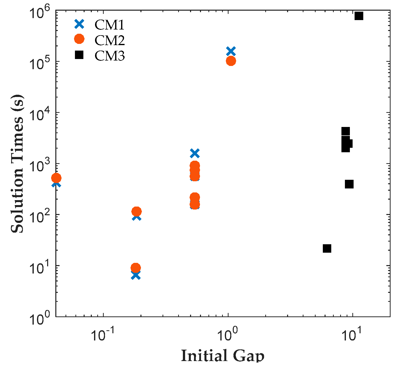
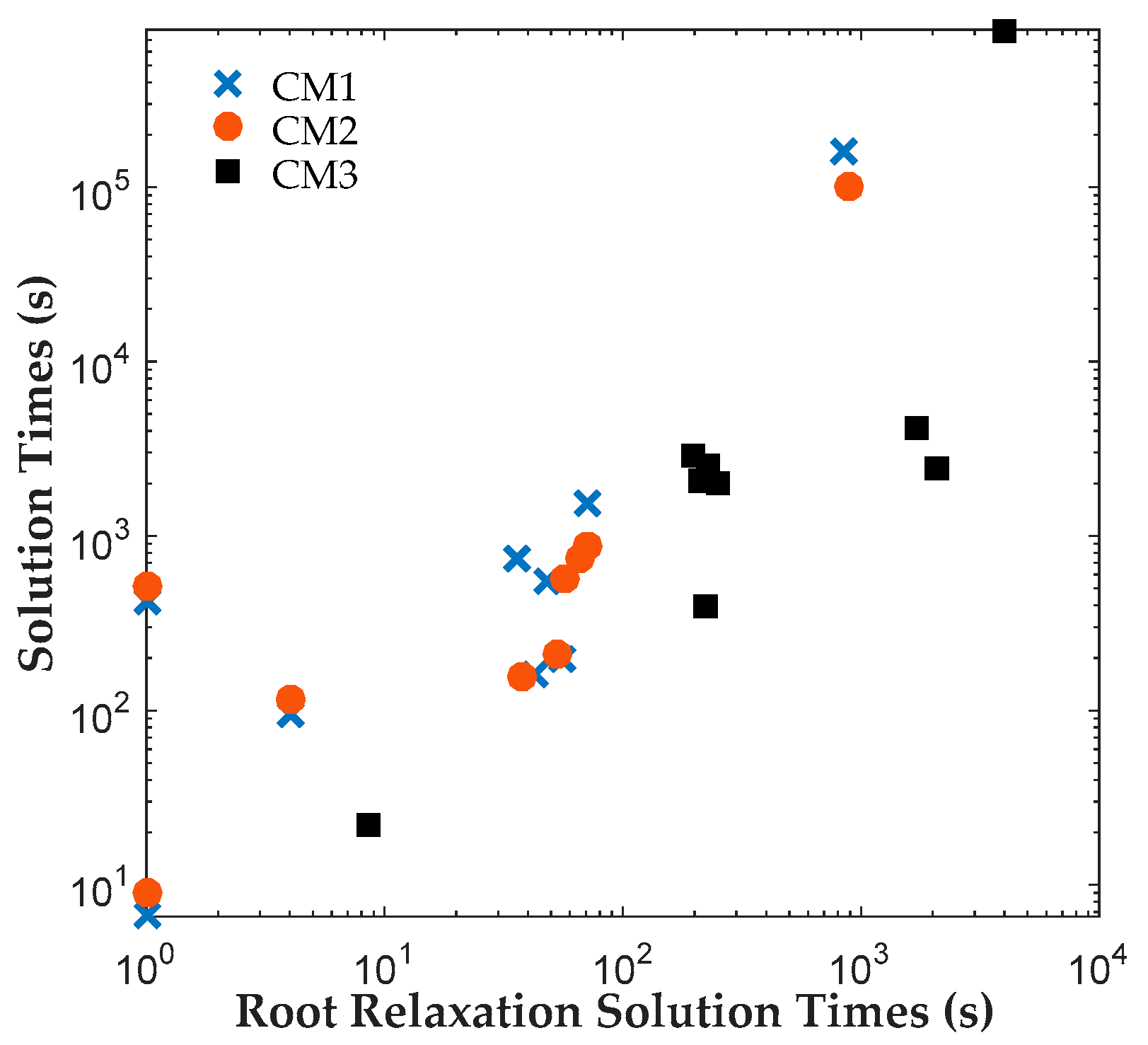
The results reveal that both CM1 and CM2 provide tighter formulations than CM3 and are solved faster by ILOG CPLEX Optimization Studio. The proposed binary variables in CM1 and CM2 contribute to shorter root relaxation solution times and generate much tighter initial gaps. It is worth noting that for all formulations, most problems were solved at the root node. For instances with branches, CM1 and CM2 consistently required fewer branches than CM3, which suggest that the binary variables in CM1 and CM2 provided ILOG CPLEX Optimization Studio a more efficient branching variable. The correlation coefficients between the solution time and root relaxation solution time, initial gap and number of branches, respectively, revealed that all three have strong positive relationship to solution times. When the root relaxation solution time, initial gap and number of branches of a case increase, so does its solution time. For all formulations, the correlations suggest that the root relaxation solution time and number of branches have stronger impact on solution time than the initial gap. We also investigated the sensitivity of solution times and problem sizes to the parameters of the clinical trial planning problem. The results revealed that the resource constraints and length of planning horizon contribute most to the computational complexity of this problem. It is worth noting that ILOG CPLEX Optimization Studio was not able to solve any of the formulations for a seven-drug case study. The future work will focus on developing decomposition approaches to generate valid upper and lower bounds quickly to solve large instances of the clinical trial planning problem.
In this paper, the outcomes of clinical trials of different drugs are assumed to be independent. This assumption may not be valid when the pipeline contains drugs that are being developed for treating similar conditions or that have similar formulations and characteristics. In such cases, the outcomes of the events for these drugs may not be independent, i.e., may be correlated. Then, the decision to start any clinical trial of these drugs will not only affect the timing of realizations of their endogenous uncertain parameters (clinical trial outcomes), but also affect the probability distributions of these uncertain parameters. For instance, let’s assume that drugs D1 and D2 have similar formulations and their outcomes are correlated and that the solution recommends starting drug trial pair (D1, PI) at period one. When the outcome of (D1, PI) is realized, the probability distribution of outcome space for D2 would be different if drug D1 passes PI or fails it. This will make the resulting problem a MSSP with both Type I and Type II endogenous uncertainty, which is a more difficult formulation to solve with limited approaches available to address it. We left this as future study.

Acknowledgments

We acknowledge the Auburn University Hopper Cluster for support of this work.

Author Contributions

This paper is a collaborative work of both authors. They both conceived the methodology; Z.Z. developed the formulations and implemented the tests in Pyomo; S.C. supervised the project and provided guidance throughout the project; Z.Z. and S.C. wrote the paper.

Conflicts of Interest

The authors declare no conflict of interest. The founding sponsors had no role in the design of the study; in the collection, analyses, or interpretation of data; in the writing of the manuscript and in the decision to publish the results.

Appendix A. Nomenclature

Indices/Sets

i ϵ Idrugs
j ϵ Jclinical trials; J = {PI, PII, PIII}
r ϵ Rresource type
s,s’ ϵ Sscenarios
p ϵ {1,2,…T}time periods
t ϵ {1,2,…T + maxijij)}time periods
Bpairs of scenarios that differ in the outcome of one clinical trials (i, j); non-anticipativity constraints are expressed only for (s,s’) ϵ B.

Parameters

Ci, jcost of trial time periods
Cdtdiscounting factor for time value of money
fi. jdiscounting factor for open revenue
Pi, jprobability of trial (i, j) being successful
psprobability of scenario s
revimaxmaximum possible revenue for drug i
revijopenestimated revenue realized for drug i, if trial (i, j − 1) completed while trial (i, j) not started, is successfully developed beyond the end of the time horizon
γiDloss coefficient—late completion
γiLloss coefficient—loss in active patent life
ρi,j,rresources of type r required to start trial (i, j)
τi, jduration of trial (i, j)
ρrmaxmaximum resources available of type r

Variables

Cststotal development cost in scenario s
Rvsrevenue of scenario s
FRvsfree revenue of scenario s
ENPVexpected net present value
Xi,j,p,s ϵ {0, 1}1 if clinical trial (i, j) starts at the time p for scenario s
Yi,j,t,s ϵ {0, 1}1 if clinical trial (i, j) ends at the time t for scenario s
Wi,j,t,p,s ϵ {0, 1}1 if clinical trial (i, j) starts at the time p and ends at the time t for scenario s
Vi,j,t,s ϵ [0, 1]1 if clinical trial (i, j) is completed by the beginning of period t in scenario s
Zi,j,t,s ϵ [0, 1]1 if clinical trial (i, j) can be started at the beginning of time t for scenario s

Appendix B. MSSP Formulation of Colvin and Maravelias (2008)

E N P V =   s p s ( R v s +   F R e v s C s t s )
V i , j , t , s = V i , j , t 1 , s + X i , j , t τ i , j , s                       i , j , t , s
Z i , 1 , 1 , s = 1 X i , 1 , t , s                   i , s
Z i , 1 , t , s = Z i , 1 , t 1 , s X i , j , t , s                         i , t > 1 , s
Z i , j , t , s =   Z i , j , t 1 , s + X i , j 1 , t τ i , j 1 , s X i , j , t , s   i ,   j > 1 , t , s
t X i , j , t , s 1             i , j , s
t t X i , j , t , s   V i , j 1 , t , s         i , j > 1 , t , s
i j t > t τ i , j t t ρ i , j , r X i , j , t , s ρ r m a x    r , t , s
X i , 1 , 1 , s = X i , 1 , 1 , 1         i , s
V i s , s , j s , s , t , s     X i , j , t , s X i , j , t , s V i s , s , j s , s , t , s     i , j ,   ( s , s ) Ψ ,   t > 1
C s t s = i , j , t c d t C i , j X i , j , t , s   s
R v s = i t r e v i m a x X i , P I I , t , s γ i D ( Z i , P I I , t , s + Z i , P I I I , t , s ) γ i L ( t + τ i , P I I I ) X i , P I I I , t , s   s
F R e v s = i j r e v i , j o p e n f i , j Z i , j , | T | , s + i j { P I , P I I } t > | T | τ i , j r e v i , j , t r u n f i , j + 1 X i , j , t , s   s
r e v i , j o p e n = r e v i m a x γ i L ( | T | + j j τ i , j )
r e v i , j r u n = r e v i m a x γ i L ( t + j j τ i , j )
f i , j = 0.9 [ r e v i m a x γ i L | T | j j C i , j r e v i m a x γ i L | T | ]
Xi,j,t,s ∈ {0,1} 1 if trial (i,j) starts at the beginning of time t for scenario s
Vi,j,t,s ∈ [0,1] 1 if trial (i,j) is completed at the beginning of time t for scenario s
Zi,j,t,s ∈ [0,1] 1 if trial (i,j) can be started at the beginning of time t for scenario s

Appendix C. The Parameters of Five Base Case

Table A1. Parameters of the two-drug case study.
DrugDurationProbability of SuccessCost ($M)Resource 1 (Max = 2)Resource 2 (Max = 3)revmaxγLγD
PIPIIPIPIIPIPIIPIPIIPIPII
D1240.30.510901112310019.244
D2230.40.610801211325019.656
Clinical trial plan for a 15-month planning horizon divided into five equal time periods.
Table A2. Parameters of the three-drug case study.
DrugDurationProbability of SuccessTrial Cost ($M)Resource 1 (Max = 2)Resource 1 (Max = 3)revmaxγLγD
PIPIIPIIIPIPIIPIIIPIPIIPIIIPIPIIPIIIPIPIIPIII
D12440.30.50.81090220112123310019.244
D22350.40.60.81080200122113325019.656
D32340.30.60.9109018011211333002052
Clinical Trial plan for a 36-month planning horizon divided into 12 equal time periods.
Table A3. Parameters of the four-drug case study.
DrugDurationProbability of SuccessTrial Cost ($M)Resource 1 (Max = 4)Resource 1 (Max = 3)revmaxγLγD
PIPIIPIIIPIPIIPIIIPIPIIPIIIPIPIIPIIIPIPIIPIII
D11130.30.50.81090220112123310019.222
D21220.40.60.81080200122113325019.628
D31130.30.60.9109018011211333002026
D41220.40.60.810100170112123300019.424
Clinical trial plan for an 18-month planning horizon divided into six equal time periods.
Table A4. Parameters of the five-drug case study.
DrugDurationProbability of SuccessTrial Cost ($M)Resource 1 (Max = 4)Resource 1 (Max = 3)revmaxγLγD
PIPIIPIIIPIPIIPIIIPIPIIPIIIPIPIIPIIIPIPIIPIII
D11130.30.50.81090220112123310019.222
D21220.40.60.81080200122113325019.628
D31130.30.60.9109018011211333002026
D41220.40.60.810100170112123300019.424
D51230.350.50.91070210112113315019.624
Clinical trial plan for an 18-month planning horizon divided into six equal time periods.
Table A5. Parameters for a six-drug case study.
DrugDurationProbability of SuccessTrial Cost ($M)Resource 1 (Max = 4)Resource 1 (Max = 3)revmaxγLγD
PIPIIPIIIPIPIIPIIIPIPIIPIIIPIPIIPIIIPIPIIPIII
D11130.30.50.81090220112123310019.222
D21220.40.60.81080200122113325019.628
D31130.30.60.9109018011211333002026
D41220.40.60.810100170112123300019.424
D51230.350.50.91070210112113315019.624
D61230.450.450.8108519512221330501925
Clinical trial plan for an 18-month planning horizon divided into six equal time periods.

Appendix D. The Parameter Perturbation Results for CM1, CM2 and CM3

Table A6. Parameter perturbation results for CM1, CM2 and CM3.
NumbersCase NameENPVSolving Times (s)
CM1CM2CM3
15-Drug-GD75%1360.783324264972
25-Drug-GD90%2127.535365513870
35-Drug-GD110%2123.034776385759
45-Drug-GD125%2127.564895325656
55-Drug-GL75%2083.532602775650
65-Drug-GL90%2083.44424404380
75-Drug-GL110%2081.133964184393
85-Drug-GL125%2080.274764526214
95-Drug-RV75%2111.884044126021
105-Drug-RV90%2093.385445545912
115-Drug-RV110%2070.034275734137
125-Drug-RV125%2051.494774794249
135-Drug-TC75%1443.153473903556
145-Drug-TC90%1826.371752143511
155-Drug-TC110%2337.794855006824
165-Drug-TC125%2721.786716024451
175-Drug-TL12003384584
185-Drug-TL2186291423

References

  1. PhRMA. Biopharmaceutical Research Industry Profile, Pharmaceutical Research and Manufacturers of America; PhRMA: Washington, DC, USA, 2016. [Google Scholar]
  2. IMS. Institute Global Use of Medicines: Outlook through 2016; Future Prescr; IMS: Parsippany, NJ, USA, 2013; Volume 14, pp. 2–10. [Google Scholar]
  3. FDA. FDA Drug Approval Process—US Food and Drug Administration. Available online: http://www.fda.gov/downloads/Drugs/ResourcesForYou/Consumers/UCM284393.pdf (accessed on 28 August 2017).
  4. FDA. The Drug Development Process—US Food and Drug Administration. Available online: https://www.fda.gov/forpatients/approvals/drugs/ucm405622.htm (accessed on 21 August 2017).
  5. Goel, V.; Grossmann, I.E. A Class of stochastic programs with decision dependent uncertainty. Math. Program. 2006, 108, 355–394. [Google Scholar] [CrossRef]
  6. Gatica, G.; Papageorgiou, L.G.; Shah, N. Capacity planning under uncertainty for the pharmaceutical industry. Chem. Eng. Res. Des. 2003, 81, 665–678. [Google Scholar] [CrossRef]
  7. Colvin, M.; Maravelias, C.T. A stochastic programming approach for clinical trial planning in new drug development. Comput. Chem. Eng. 2008, 32, 2626–2642. [Google Scholar] [CrossRef]
  8. Colvin, M.; Maravelias, C.T. Scheduling of testing tasks and resource planning in new product development using stochastic programming. Comput. Chem. Eng. 2009, 33, 964–976. [Google Scholar] [CrossRef]
  9. Colvin, M.; Maravelias, C.T. Modeling methods and a branch and cut algorithm for pharmaceutical clinical trial planning using stochastic programming. Eur. J. Oper. Res. 2010, 203, 205–215. [Google Scholar] [CrossRef]
  10. Sundaramoorthy, A.; Evans, J.M.B.; Barton, P.I. Capacity planning under clinical trials uncertainty in continuous pharmaceutical manufacturing, 1: Mathematical framework. Ind. Eng. Chem. Res. 2012, 51, 13692–13702. [Google Scholar] [CrossRef]
  11. Solak, S.; Clarke, J.P.B.; Johnson, E.L.; Barnes, E.R. Optimization of R&D project portfolios under endogenous uncertainty. Eur. J. Oper. Res. 2010, 207, 420–433. [Google Scholar]
  12. Gupta, V.; Grossmann, I.E. A new decomposition algorithm for multistage stochastic programs with endogenous uncertainties. Comput. Chem. Eng. 2014, 62, 62–79. [Google Scholar] [CrossRef]
  13. Christian, B.; Cremaschi, S. Heuristic solution approaches to the pharmaceutical R&D pipeline management problem. Comput. Chem. Eng. 2015, 74, 34–47. [Google Scholar]
  14. Christian, B.; Cremaschi, S. A branch and bound algorithm to solve large-scale multistage stochastic programs. In Proceedings of the FOCAPO/CPC, Tuscan, AZ, USA, 8–12 January 2017. [Google Scholar]
  15. Apap, R.M.; Grossmann, I.E. Models and computational strategies for multistage stochastic programming under endogenous and exogenous uncertainties. Comput. Chem. Eng. 2017, 103, 233–274. [Google Scholar] [CrossRef]
  16. Christian, B.; Cremaschi, S. Variants to a knapsack decomposition heuristic for solving R&D pipeline management problems. Comput. Chem. Eng. 2017, 96, 18–32. [Google Scholar]
  17. Zeng, Z.; Cremaschi, S. Artificial lift infrastructure planning for shale gas producing horizontal wells. In Proceedings of the FOCAPO/CPC, Tuscan, AZ, USA, 8–12 January 2017. [Google Scholar]
  18. Hart, W.E.; Laird, C.; Watson, J.P.; Woodruff, D.L. Pyomo–Optimization Modeling in Python; Springer Science & Business Media: New York, NY, USA, 2012; Volume 67. [Google Scholar]
  19. Auburn University. Hopper Cluster. Available online: https://hpcportal.auburn.edu/hpc/2016_cluster.php (accessed on 12 September 2017).
Figure 1. The outcome space of uncertain parameter associated with drug i, Ω i .
Processes 05 00071 g001
Figure 2. Comparison of scheduling variables in CM1, CM2 and CM3 formulations.
Processes 05 00071 g002
Figure 3. Multi-stage decisions in the optimal solution.
Processes 05 00071 g003
Figure 4. Change in solution times of CM1, CM2 and CM3 with number of drugs.
Processes 05 00071 g004
Figure 5. Comparison of (a) solution times, (b) root relaxation solution times, (c) initial gaps, and (d) number of branches for CM1, CM2 and CM3.
Processes 05 00071 g005
Figure 6. Change in solution times with root relaxation solution time for CM1, CM2 and CM3. The strong linear correlation is evident from this plot.
Processes 05 00071 g006
Figure 7. Change in solution times with changes in initial gaps of CM1, CM2 and CM3. Initial gaps of CM1 and CM2 are consistently smaller than CM3.
Processes 05 00071 g007
Figure 8. Change in solution times with the number of branches needed to solve CM1, CM2 and CM3. Please note most problems are solved at the root node, and when branching is required to solve the problem, the linear dependency of solution time to number of branches required to solve the problem is evident from this figure.
Processes 05 00071 g008
Table 1. Problem sizes for five instances of CM1, CM2 and CM3.
CasesCM1CM2CM3
VariablesConstraintsVariablesConstraintsVariablesConstraints
2-Drug58695283814926131051
3-Drug17,28144,06524,19364,80121,24949,761
4-Drug48,385138,49766,817193,79357,345150,529
5-Drug239,617802,305454,6571,078,785284,673862,721
6-Drug1,142,7854,386,8171,585,1535,713,9211,359,8734,677,633
Table 2. Descriptions of case studies used to study the impact of problem parameters on solution times of CM1, CM2 and CM3.
VariationCase NameVariation Value
Resource availability5-Drug-
5-Drug-RA40%+40%
5-Drug-RA70%+70%
5-Drug-RA100%+100%
Trial cost5-Drug-TC75%−25%
5-Drug-TC90%−10%
5-Drug-TC110%+10%
5-Drug-TC125%25%
Maximum revenue5-Drug-RV75%−25%
5-Drug-RV90%−10%
5-Drug-RV110%+10%
5-Drug-RV125%+25%
Active patent life loss penalty5-Drug-GL75%−25%
5-Drug-GL90%−10%
5-Drug-GL110%+10%
5-Drug-GL125%+25%
Market share loss penalty5-Drug-GD75%−25%
5-Drug-GD90%−10%
5-Drug-GD110%+10%
5-Drug-GD125%+25%
Trial Duration5-Drug-TL1+1
5-Drug-TL2+2
Table 3. Resource constraint perturbation results for CM1, CM2 and CM3.
CasesENPVSolution Time (CPUs)
CM1CM2CM3
3-Drug11897510
3-Drug-R40%12115418
3-Drug-R70%1220225
3-Drug-R100%1221224
4-Drug169781128
4-Drug-R40%1719348
4-Drug-R70%1721346
4-Drug-R100%1721345
5-Drug20831611582372
5-Drug-R40%21233743324
5-Drug-R70%21282532153
5-Drug-R100%21285972318
6-Drug245012,9918114108,746
6-Drug-R40%2510649688.59786
6-Drug-R70%25172973343629
6-Drug-R100%251728232343348
Table 4. Size perturbation cases and file names with variation value.
Case NumberVariationMagnitude of Change
1Number of trials+1
2+2
3Number of resources+1
4+2
5+3
6+4
7Length of planning horizon−2
8Original 5-Drug Case+2
90

