Combined Noncyclic Scheduling and Advanced Control for Continuous Chemical Processes

Abstract

A novel formulation for combined scheduling and control of multi-product, continuous chemical processes is introduced in which nonlinear model predictive control (NMPC) and noncyclic continuous-time scheduling are efficiently combined. A decomposition into nonlinear programming (NLP) dynamic optimization problems and mixed-integer linear programming (MILP) problems, without iterative alternation, allows for computationally light solution. An iterative method is introduced to determine the number of production slots for a noncyclic schedule during a prediction horizon. A filter method is introduced to reduce the number of MILP problems required. The formulation’s closed-loop performance with both process disturbances and updated market conditions is demonstrated through multiple scenarios on a benchmark continuously stirred tank reactor (CSTR) application with fluctuations in market demand and price for multiple products. Economic performance surpasses cyclic scheduling in all scenarios presented. Computational performance is sufficiently light to enable online operation in a dual-loop feedback structure.

1. Introduction

Production scheduling and advanced control are terms which describe efforts to optimize chemical manufacturing operations. Production scheduling seeks to optimally pair production resources with production demands to maximize operational profit. Advanced controls seek to optimally control a chemical process to observe environmental and safety constraints and to drive operations to the most economical conditions. Model predictive advanced controls use process models to make predictions into a future horizon based on possible control moves to determine the optimal sequence of control moves to meet an objective, such as reaching an operational set point. In a multi-product continuous chemical process, steady-state operational set points or desired operational conditions over a future time horizon are determined by the production schedule, determining at which times, in what amounts, and in which sequence certain products should be produced.

As scheduling and advanced control are closely interrelated, both seeking to optimize chemical manufacturing efficiency over future time horizons, their integration has been the subject of significant recent investigation. Multiple review articles have been published on the integration of scheduling and control [1,2,3,4]. As schedules are informed of process dynamics as dictated by control structure and process nonlinearities, schedules produced become more aligned with actual process operations and schedule efficacy improves [5]. Conversely, when scheduling and advanced control are separated, coordination of closed-loop responses to process disturbances is lost, unrealistic set points may be passed from scheduling to advanced controls, and advanced control may seek to drive the process to sub-optimal operating conditions due to a lack of communication [3,5,6]. In the presence of a process disturbance, for example, advanced controls may attempt to return to a set point determined prior to the disturbance, whereas a recalculation of the schedule from the measured disturbed state, with knowledge of process dynamics and controller behavior, may show a different schedule and set point to be most economical [5,7].

One setback to the integration of scheduling and control is computational difficulty. Advanced controls, particularly model predictive controls, utilize dynamic process models in dynamic optimization problems, forming linear programming (LP) or nonlinear programming (NLP) optimization problems depending on the type of model used. Scheduling involves discrete or binary decisions, such as assigning particular products to production at given times. This gives rise to mixed-integer programming problems for scheduling. When scheduling and control are combined, the computational burden of mixed-integer programming is combined with the LP or NLP dynamic optimization problems. Additionally, dynamic optimization control problems are not required to be solved only once, as in an iteration of advanced online control, but for each grade transition during a production schedule. The integrated scheduling and control (ISC) problem has been shown to be computationally difficult, and much research has been invested in decomposition and reduction of computational burden for the problem [8,9,10,11,12].

Reduction of the computational burden of integrated scheduling and control is especially important for enabling online implementations. It has been shown repeatedly in simulation that closed-loop online implementations of integrated scheduling and control are critical to recalculating optimal scheduling and control when faced with process disturbances [5,7]. Additionally, it has been demonstrated that online closed-loop integrated scheduling and control is vital to optimally responding to variable market conditions, including demand fluctuations and price fluctuations [5,13,14]. As mentioned in review articles on integrated scheduling and control, a key motivator for integration is the reduced time-scale at which market conditions fluctuate [1,2]. A reduced time-scale for market fluctuations implies that the time-scale at which the economically optimal schedule and associated optimal control profile fluctuates is likewise reduced. Thus, online recalculation to respond to market condition updates is critical to integrated scheduling and control, and computational burden reduction to enable such implementation is a salient topic for researchers.

Online responsiveness to volatile market conditions can improve process economics by updating or changing the existing schedule [5]. The majority of integrated scheduling and control formulations have used cyclic schedules [7,8,9,10,11,15,16,17,18,19,20,21,22]. However, it has been suggested that a dynamic cyclic schedule may improve process economics [23]. Beal et al. suggest that a dynamic cyclic schedule can increase the flexibility of scheduling beyond the rigidity of a cyclic product grade wheel. A dynamic cyclic schedule can dynamically change the sequence and duration of production of products on the grade wheel based on process disturbances, sudden surges in demand for specific products, or time-dependent constraints such as operator availability for equipment handling. Economic benefit from dynamic cyclic scheduling has been demonstrated in previous work [5,7]. Recent developments in integrated scheduling and control with discrete representations of time do away with the idea of a cyclic schedule as the schedule is determined as a sum total of the binary production variables at each discrete point in time during a prediction horizon [24]. In these works, the number of products manufactured, the selection of manufactured products, sequence, and timing are all solved simultaneously with process dynamic models, resulting in a computationally heavy formulation. Evidence of benefits from noncyclic scheduling has also been demonstrated in other fields, such as cluster-tool robot scheduling for semiconductor fabrication [25,26,27,28,29,30].

This work explores fully noncyclic scheduling integrated with advanced process control. A continuous representation of time is utilized for the scheduling model, and nonlinear model predictive control (NMPC) is utilized for advanced process control. A decomposition is utilized to break the problem into NLP problems and mixed-integer linear programming (MILP) problems without the need for alternating iterations. Further decomposition into problems calculated offline from information known a priori with results stored in memory and problems solved online further reduce the computational burden of integrated scheduling and control, making the problem feasible for online, closed-loop implementation. Noncyclic scheduling is implemented through an iterative method, which iterates through potential numbers of products to produce during a future horizon. The integrated scheduling and control algorithm selects the number of products to manufacture, which products to manufacture, the production sequence, production timing and amounts, as well as the grade transitions between each product. This allows greater flexibility than cyclic scheduling for responding to variable product demands and prices.

2. Literature Review

Extensive prior research has been conducted on integrated scheduling and control, including several literature review articles [1,2,3,4,31,32]. Mahadevan et al. incorporate control level considerations such as grade transition costs in production scheduling [33]. Grossman and Flores-Tlacuahuac investigate simultaneous cyclic scheduling and process control for continuously stirred tank reactors (CSTR), polymer manufacturing processes, and for parallel continuous chemical processes [16,17,34]. A mixed-integer dynamic optimization (MIDO) approach has been used to solve the simultaneous continuous-time scheduling and optimal control problem with orthogonal collocation on finite elements. The large MIDO problem is initialized with dynamic optimization grade transition problem solutions [17]. Chatzidoukas et al. study solving the simultaneous dynamic optimization optimal grade transitions and scheduling problem for fluidized-bed reactors (FBR) via a MIDO approach with orthogonal collocation on finite elements [35]. They also study simultaneous selection of closed-loop controllers and selection of controller parameters with the scheduling problem for polymerization processes [36,37]. Terrazas-Moreno and Flores-Tlacuahuac also investigate simultaneous cyclic scheduling and control of continuous chemical processes, and study a langrangean heuristic method for reduction of computational burden [15,18]. Baldea et al. and Du et al. demonstrate reduction of computational burden of the integrated problem by using reduced order, or scale-bridging models (SBM), in scheduling [8,21]. Scale-bridging models encapsulate the core information about process dynamics in a low-order model for integrated solution with scheduling [8,9,21]. Nie et al. study the short-term scheduling and dynamic optimization of multi-unit chemical processes using a state equipment network (SEN) and mixed-logic dynamic optimization (MLDO), solved by a Big M reformulation and orthogonal collocation into an MINLP problem [38]. Nie et al. also study combined scheduling and control of parallel reactors using a resource task network (RTN) coupled with dynamic models [39]. The solution is achieved by iteration between MILP and NLP subproblems and Benders’ decomposition. Gutierrez-Limon et al. develop a multi-objective optimization approach for simultaneous scheduling and control of continuous chemical processes [40]. Benefit is demonstrated from using multi-objective approaches with Pareto fronts rather than combining economic and dynamic performance objectives into a single objective function. Gutierrez-Limon and Flores-Tlacuahuac also investigate simultaneous planning, scheduling, and control for continuous chemical processes using a large MINLP problem and NMPC [41]. Prata et al. study the use of outer approximation methods for the solution of integrated scheduling and control problems [42].

Zhuge and Ierapetritou investigate closed-loop implementation of integrated scheduling and control. The benefit of integrated scheduling and control responsive to process disturbances in continuous chemical processes is demonstrated [7]. Further work by Zhuge and Ierapetritou investigates various methodologies for the reduction of computational burden for integrated scheduling and control to enable feasible online implementation. Application of multi-parametric model predictive control (mp-MPC) to shift the solution of optimal control dynamic optimization problems offline while using only an explicit control solution with minimal computational requirements is studied [22]. The explicit control solution from mp-MPC is integrated with scheduling to reduce the computational requirements of the online problem. A simplified piece-wise affine (PWA) model to represent process dynamics for the scheduling level, rather than a first-principles process model, and fast model predictive control (fast MPC) at the control level are implemented, resulting in a significant reduction of computational burden. Additionally, a decomposition approach is presented based on optimality analysis showing that production sequence and transition times are independent of product demands [20]. The transition stages, a smaller-scale mixed-integer nonlinear programming (MINLP) problem, are solved separately from the production stages, a smaller-scale NLP problem, as opposed to solving an integrated large-scale MINLP problem. No need for iterative alternation is necessary between the two smaller scale problems.

Chu and You also investigate closed-loop implementations of integrated scheduling and control. They investigate solutions through mixed-integer fractional programming (MINFP) with a fast, global optimization algorithm in a simultaneous controller selection and scheduling problem for online implementation [10,11]. They also investigate multi-objective optimization, including decomposition into an offline solution of the Pareto frontier and an online MINLP problem simultaneously selecting a batch scheduling recipe and optimal control [43]. Chu and You also investigate two-stage stochastic programming to confront uncertainty in integrated scheduling and control problems; however, the problem is computationally difficult [44]. Reduction of computational difficulty via nested Benders’ decomposition is investigated. They also investigate a decomposition into a master scheduling problem (MILP) and a primal problem containing multiple separable dynamic optimization (or control) problems [45]. The primal and master problems are solved together via iterative alternation until convergence to an acceptable error is achieved. Nystrom et al. also examine the use of iterations between master MILP problems and primal NLP problems until convergence to an acceptable error is achieved for the solution of integrated scheduling and control problems [46,47]. Chu and You also investigate integration of planning, scheduling, and control in a large MIDO problem discretized into a MINLP problem by orthogonal collocation on finite elements. They use surrogate models to effectively reduce the computational burden for the large problem. A decomposition into a leading scheduling problem and following dynamic optimization problems based on Stakelberg game theory is also investigated [48].

Rossi has recently demonstrated a decomposition of integrated scheduling and control for batch processes [49]. The schedule is calculated offline but is updated in real time by updates from an online optimal control problem. Bauer et al. has recently suggested that key performance indicators (KPI) are already implemented in industry as the integrating factor between scheduling and control. Scheduling and control for economic model predictive control (EMPC) of buildings with energy storage has been investigated [50].

Integration of design, scheduling, and control has also been investigated. Terrazas-Moreno and Flores-Tlacuahuac examine combined design, scheduling, and control with dynamic process models nearly a decade ago [51]. Koller et al. present an optimization framework for integrated scheduling, control, and design of multi-product processes with uncertainty. Worst-case scenarios are examined in the algorithm to design a process feasible under all worst-case scenarios [52]. Grade transitions and scheduling are incorporated via flexible finite elements and dynamic process models. Patil et al. study combined design, scheduling, and control for continuous processes [53]. They study worst-case scenarios through frequency response analysis and apply their formulation to a high impact polystyrene (HIPS) polymerization process.

Moving horizon implementations of closed-loop integrated scheduling and control have been studied by various researchers. Chu and You use a moving future horizon for online recalculation of integrated scheduling and control for batch processes in the presence of disturbances such as unit breakdowns and system disruptions and a dual feedback structure to reduce the frequency of integrated problem solution [12]. Pattison et al. investigate using a scale-bridging model (SBM) in a closed-loop moving horizon implementation of integrated scheduling and control for an industrial air separation unit (ASU), demonstrating effective response to planned maintenance, unplanned maintenance, and random failure scenarios [14]. A heuristic reactive strategy for integrated planning, scheduling, and control for multi-product continuous chemical processes has been developed and applied in scenarios with market updates with fluctuating product demands [54].

3. Problem Formulation

This work investigates integration of scheduling and control with noncyclic scheduling and NMPC. The algorithm is allowed to select the number of products to manufacture during a prediction horizon, which products to manufacture, the production sequence, production durations, and optimal control moves. The mathematical formulation is presented in this section.

3.1. Decomposition

An objective of this work is feasibility for closed-loop online implementation. To accomplish this objective, the problem is decomposed into an MILP programming problem and multiple separable NLP dynamic optimization, or optimal control, problems without the need for alternating iterations. This formulation builds on previous work that demonstrates the separability of the integrated scheduling and control problem into subproblems without the need for iterations [20] and builds on previous work which demonstrates the separation into MILP and dynamic optimization problems [10,46,47]. This formulation also builds on previous work that demonstrates benefits from shifting separable computational burden into offline portions of the integrated problem [11,19,22,55].

The main decomposition employed in this work is a decomposition into an MILP problem that determines the production sequence and production amounts for each manufactured product, and a group of separable dynamic optimization NLP problems for optimal control during grade transitions. The formulation for the MILP problem is as follows:

$$\begin{array}{cc}\hfill \underset{{\omega }_i,z_{i,s},t_i^s,t_i^f\forall i,s}{max}& J=\sum _{i=1}^n{\mathrm{\Pi }}_i{\omega }_i-\sum _{i=1}^n{c}_{storage,i}{\omega }_i\sum _{s=1}^m{z}_{i,s}(T_M-t_s^f)-W_{\tau }\sum _{s=1}^m{\tau }_s,\hfill \\ \hfill \mathrm{s}.\mathrm{t}.& \mathrm{Equations}\left(2\right)–\left(8\right),\hfill \end{array}$$

(1)

where $T_M$ is the makespan, n is the number of products, m is the number of slots (constrained to equal the number of products such that $m=n$), $z_{i,s}$ is the binary variable that governs the assignment of product i to a particular slot s, $t_s^s$ is the start time of the slot s, $t_s^f$ is the end time of slot s, ${\mathrm{\Pi }}_i$ is the per unit price of product i, $W_{\tau }$ is an optional weight on grade transition minimization, ${\tau }_s$ is the transition time within slot s, $c_{storage,i}$ is the per unit cost of storage for product i, and ${\omega }_i$ represents the amount of product i manufactured,

$${\omega }_i=\sum _{s=1}^m{\int }_{t_s^s+{\tau }_s}^{t_s^f}{z}_{i,s}qdt.$$

(2)

Products are assigned to each slot using a set of binary variables, $z_{i,s}\in \left\{0,1\right\}$ that assign a product i to be produced in a given slot s. Constraints of the following form are added:

$$\sum _{i=1}^n{z}_{i,s}=1\forall s,$$

(3)

which limit the assignment of production within each slot, ensuring that one and only one product is assigned to each slot, and

$$\sum _{s=1}^m{z}_{i,s}\le 1\forall i,$$

(4)

which constrains the production of products. This constraint, unlike traditional continuous-time scheduling formulations, does not require each product to be produced once and only once during the schedule, but allows the optimization to select the number of products to produce during the horizon for scheduling provided each slot has a production assignment (Equation (3)). Not every available product must be produced during each schedule.

The values of the vector ${\tau }_s$ are determined by the optimization variables $z_{i,s}$. ${\tau }_s$ represents the transition time between the product made in slot s− 1 and product made in slot s. Thus, the value of ${\tau }_s$ is determined by the optimal values of $z_{j,s-1}$ and $z_{k,s}$ which determine which products are assigned to slots $s-1$ and s. For $z_{j,s-1}$ and $z_{k,x}$, ${\tau }_s$ would be equal to the calculated grade transition time from product j to product k. The possible values for ${\tau }_s$ are the grade transition times calculated via NLP optimal grade transition problems (Equation (9)). The time points must satisfy the precedence relations:

$$t_s^f>t_s^s+{\tau }_s\forall s>1,$$

(5)

$$t_s^s=t_{s-1}^f\forall s\ne 1,$$

(6)

$$t_m^f=T_M,$$

(7)

which require that a time slot be longer than the corresponding transition time, impose the coincidence of the end time of one time slot with the start time of the subsequent time slot, and define the relationship between the end time of the last time slot ($t_n^f$) and the total makespan or horizon duration ($T_M$).

The makespan is fixed to an arbitrary horizon for scheduling. Demand constraints restrict production from exceeding the maximum demand (${\delta }_i$) for a given product, as follows:

$${\omega }_i\le {\delta }_i\forall i.$$

(8)

The continuous-time scheduling optimization (or MILP problem) requires transition times between steady-state products (${\tau }_{i^{\prime }i}$) as well as transition times from the current state to each steady-state product if initial state is not at steady-state product conditions (${\tau }_{0^{\prime }i}$). These grade transitions comprise the separable dynamic optimization problems or NLP portion of the overall problem decomposition.

Grade transition profiles are optimized using the following objective:

$$\begin{array}{cc}\hfill \underset{u}{min}& J={(x-x_{sp})}^T{W}_{sp}(x-x_{sp})+\Delta u^T{W}_{\Delta u}+u^T{W}_u,\hfill \\ \hfill \mathrm{s}.\mathrm{t}.& \mathrm{nonlinear}\mathrm{process}\mathrm{model},\hfill \\ & x\left(t_0\right)=x_0,\hfill \end{array}$$

(9)

where $W_{sp}$ is the weight on the set point for meeting target product steady-state, $W_{\Delta u}$ is the weight on restricting manipulated variable movement, $W_u$ is the cost for the manipulated variables, u is the vector of manipulated variables, $x_{sp}$ is the target product steady-state, and $x_0$ is the start process state from which the transition time is being estimated. The transition time is taken as the time at which and after which $|x-x_{sp}|<ϵ$, where $ϵ$ is a tolerance for meeting product steady-state operating conditions. This formulation harnesses knowledge of nonlinear process dynamics in the system model to find an optimal trajectory and minimum time required to transition from an initial concentration to a desired concentration. The usage of NMPC for grade transitions in the integrated problem effectively captures the actual behavior of the controller used in the process, as the transition times are estimated by a simulation of actual controller implementation on a first-principles nonlinear model of the process.

Because product steady-state operating conditions can be known a priori, all grade transition times between production steady-state operating conditions can be calculated offline and stored in memory in a grade transition time table: ${\tau }_{ss}$. The online portion of the NLP subproblem is comprised only of the calculation of ${\tau }_{\theta }$, the transition duration and corresponding optimal control profile from current measured state ($x_{\theta }$) and each steady-state operating condition, or, in other words, the vector of possible transitions for the first slot ($s=0$). For example, consider the case of three products as described in

Table 1. Product specifications.

Product	${\mathit{C}}_{\mathit{A}}$ (mol/L)
1	0.10
2	0.30
3	0.50

. As product steady-state conditions are known a priori as shown in Table 1, the transition times between product steady-states can be calculated through NLP problems (Equation (9)) and stored in a grade transition time table prior to operation (

Table 2. Transition time table (${\tau }_{ss}$) *.

Start	End Product
Product	1	2	3
1	0.00	0.71	1.20
2	0.45	0.00	0.71
3	0.94	1.57	0.00

* Transition times in hours.

). However, before operation, process state measurements ($x_{\theta }$) cannot be known. For example, if in the three product case described in Table 1 a process disturbance was measured at $x_{\theta }=0.19$ mol/L during online operation, for an optimal rescheduling beginning from current state $x_{\theta }$ to be calculated, transition durations from $x_{\theta }$ to each operating steady-state would need to be estimated online by solving n separable NLP optimal grade transition problems, where n is the number of steady-state products considered. The results of these online optimal transition problems would be the vector ${\tau }_{\theta }$ (

Table 3. Initial transitions (${\tau }_{\theta }$).

Product	${\mathit{\tau }}_{\mathit{\theta }}\left(\mathit{h}\right)$
1	0.31
2	0.43
3	0.96

). These transitions would be the possible values for ${\tau }_s$ for the first slot ($s=0$) in Equation (1) for the MILP rescheduling problem.

With ${\tau }_{ss}$ and ${\tau }_{\theta }$ grade transition information, the MILP problem is equipped to optimally select the production sequence and amounts for the prediction horizon based on product demands, prices, transition durations, raw material cost, storage cost, and other economic parameters. Even when a process disturbance is encountered and measured, the schedule can be optimally recalculated from the measured disturbance, $x_{\theta }$, via the incorporation of transitions from $x_{\theta }$ to each production steady-state condition (${\tau }_{\theta }$).

3.2. Iterative Method

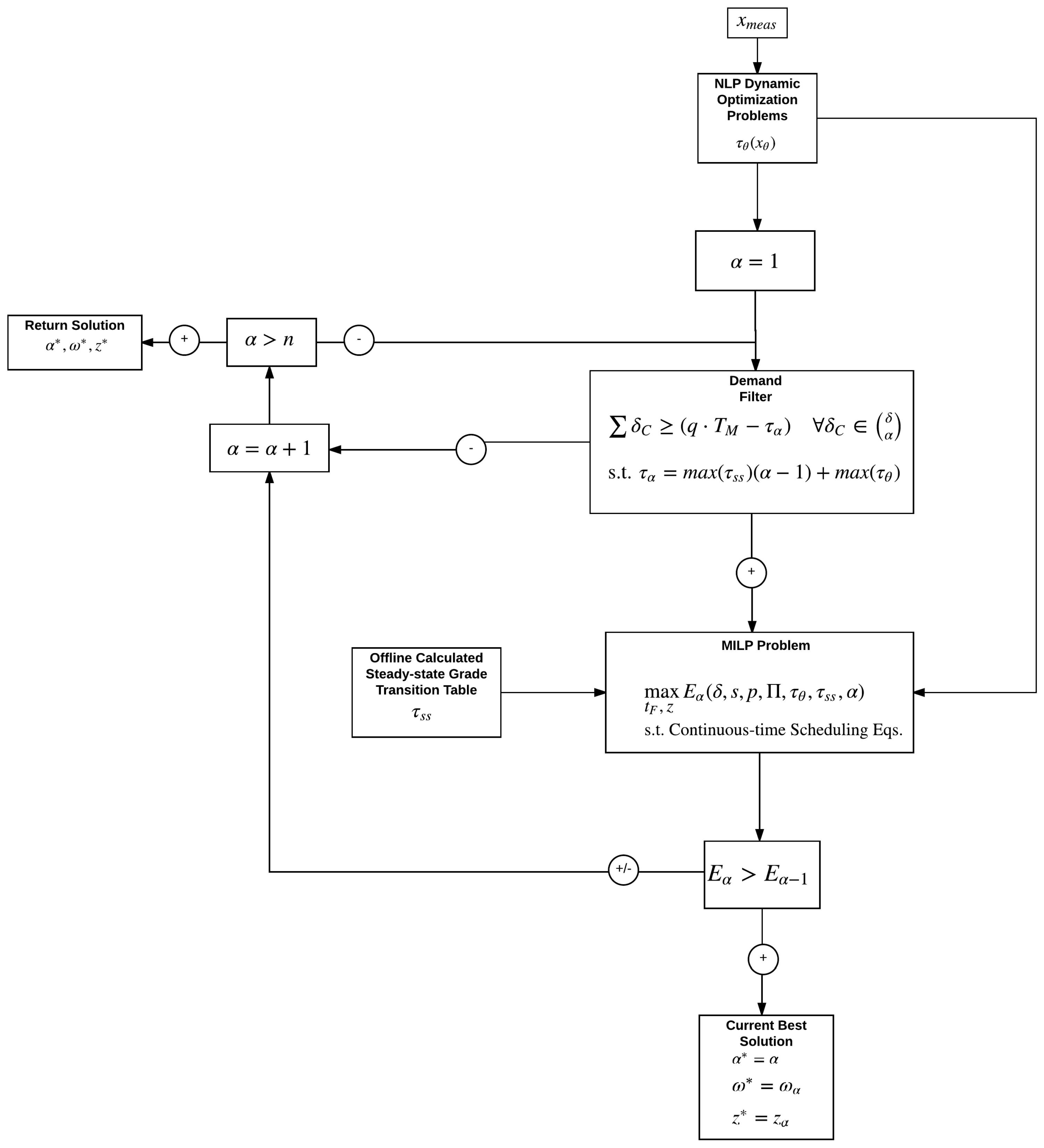
The cyclic continuous-time scheduling formulation is sub-optimal if the number of products on the wheel exceeds the optimal number of products to produce in a prediction horizon. The number of slots in the MILP problem is constrained to be equal to the number of products, causing the optimization to always create n production slots and n transitions even in cases in which <n slots would be most economical in the considered horizon for scheduling and control. To allow greater flexibility, an iterative method is introduced which leverages the computational lightness of the separated MILP subproblem. The number of slots in the continuous-time schedule is selected iteratively based on improvement to the objective function (profit), beginning from one slot, or only one product to produce during the horizon (Figure 1). The iterations begin from one slot ($\alpha =1$) due to the nature of grade transitions. Reducing the number of production slots reduces the number of necessary grade transitions, and reduces the corresponding amount of waste material produced. All grade transition NLP subproblems are calculated prior to slot iterations as grade transition information is independent of the number of production slots. This iterative method enables a noncyclic approach to combined scheduling and control and enables response to market fluctuations in product maximum demand and product price.

A heuristic demand filter is introduced to further reduce computational burden (Figure 1). The filter checks for any combination of $\alpha$ products with summed demand sufficient to fill the prediction horizon for scheduling and control. This effectively filters each possible $\alpha$ for sufficient demand before the MILP problem is executed. In calculating the minimum summed demand which must be met for the given iteration for the MILP problem to be executed, the filter accounts for transition times calculated by NLP dynamic optimization problems both offline (all ${\tau }_{i,i}$ stored in ${\tau }_{ss}$) and online (all ${\tau }_0$ stored in ${\tau }_{\theta }$). The demand must be sufficient to fill the production potential of the prediction horizon, which equates to ($q·T_M-{\tau }_{\alpha }$), where ${\tau }_{\alpha }$ is the summed grade transition durations. To ensure each $\alpha$ which has potential for sufficient demand is tested in the MILP problem, the demand filter overestimates for transition times. In the case of underestimation of total transition times (${\tau }_{\alpha }$), the demand required to fill production during the prediction horizon ($q·T_M-{\tau }_{\alpha }$) will be overestimated. In a such case, a combination ${\delta }_C$ which would have had enough demand may inaccurately be deemed insufficient. Since often the optimal number of slots will be the smallest number of slots with sufficient demand (because the number of grade transitions and the corresponding amount of off-specification production increases with the number of slots), it is pertinent to not underestimate the durations of grade transitions. To eliminate such underestimation, the maximum transitions are used for estimations of the total transition time during the prediction horizon (${\tau }_{\alpha }$).

4. Case Study Application

In this section, the performance of the iterative noncyclic integrated scheduling and control formulation in this work is demonstrated. The test scenarios and computational, economic, and closed-loop performance results of the algorithm are presented.

4.1. Process Model

This section presents the CSTR problem used to highlight the value of the formulation introduced in this work. The CSTR model is a general test problem that is widely applicable in various industries from petrochemicals to food processing. The model shown in Equations (10) and (11) is an example of an exothermic, first-order reaction of $A\Rightarrow B$ where the reaction rate is defined by an Arrhenius expression and the reactor temperature is controlled by a cooling jacket:

$$\frac{d{C}_A}{dt}=\frac{q}{V}(C_{A0}-C_A)-k_0{e}^{-E_A/RT}{C}_A,$$

(10)

$$\frac{dT}{dt}=\frac{q}{V}(T_f-T)-\frac{1}{\rho C_p}{k}_0{e}^{\frac{-E_A}{RT}}{C}_A\Delta H_r-\frac{UA}{V\rho C_p}(T-T_c).$$

(11)

In these equations, $C_A$ is the concentration of reactant A, $C_{A0}$ is the feed concentration, q is the inlet and outlet volumetric flowrate, V is the tank volume ($q/V$ signifies the residence time), $E_A$ is the reaction activation energy, R is the universal gas constant, $UA$ is an overall heat transfer coefficient times the tank surface area, $\rho$ is the fluid density, $C_p$ is the fluid heat capacity, $k_0$ is the rate constant, $T_f$ is the temperature of the feed stream, $C_{A0}$ is the inlet concentration of reactant A, $\Delta H_r$ is the heat of reaction, T is the temperature of reactor and $T_c$ is the temperature of cooling jacket. The parameters for the CSTR in this work are detailed in

Table 5. Reactor parameter values.

Parameter	Value
V	100 m${}^3$
$E_A/R$	8750 K
$\frac{UA}{V\rho C_p}$	2.09 s${}^{-1}$
$k_0$	7.2 × 10${}^{10}$ s${}^{-1}$
$T_f$	350 K
$C_{A0}$	1 mol/L
$\frac{\Delta H_r}{\rho C_p}$	−209 K m${}^3$/mol
q	100 m${}^3$/h

.

A single CSTR can make multiple products by varying the concentrations of A and B in the outlet stream, which can be done by manipulating the cooling jacket temperature $T_c$. The cooling jacket temperature is bounded by 200 K $\le T_c\le$ 500 K and a constraint on movement is added as $\Delta T_c\le 2$ K/min.

4.2. Scenarios

Five illustrative scenarios are presented to demonstrate the abilities of the noncyclic scheduling and control algorithm presented in this work, with one additional scenario introduced in Section 5 to illustrate an aspect of the iterative algorithm. The first two scenarios demonstrate the flexibility afforded by the noncyclic formulation in selecting the number of production slots and the products for production during a prediction horizon. The last three scenarios demonstrate the closed-loop performance of this formulation with process disturbances and market fluctuations. It is noted that the closed-loop performance of this formulation is also demonstrated in another work [5]; however, closed-loop selection of variable production slots is not demonstrated in another work. Additionally, analysis of computational time and comparison to a cyclic scheduling formulation are not analyzed in the companion work. All scenarios in this work use a 48 h prediction horizon, a raw material cost of $20/m${}^3$, and a flat storage cost of $0.10/m${}^3$/hr for all products. Slot times are given by the solutions returned by the optimization (${\omega }^{\ast },z^{\ast },{\alpha }^{\ast }$).

The first scenario as shown in

Table 6. Scenario 1: Product specifications.

Product	${\mathit{C}}_{\mathit{A}}$ (mol/L)	Max Demand (m${}^3$)	Price ($/m${}^3$)
1	0.10	2000	24
2	0.15	2000	29
3	0.22	2000	26
4	0.28	2000	23
5	0.34	2000	21
6	0.44	2000	21
7	0.50	2000	20

is formulated to demonstrate the flexibility of the noncyclic scheduling and control formulation. Seven products, all with large demands, are available. The noncyclic schedule is predicted to be able to select the optimal number of production slots and produce the most profitable products in the optimal production sequence rather than producing all available products in a cyclic grade wheel. The starting concentration for Scenario 1 is $C_A=0.10$ mol/L, the steady-state concentration for Product 1.

The second scenario contains comparatively less demand per available product and is expected to produce a larger number of products than in Scenario 1. The starting concentration for Scenario is $C_A=0.10$ mol/L, the steady-state concentration for Product 1. The third scenario is formulated with the same product demands and prices as in Scenario 2 (

Table 7. Scenario 2: Product specifications.

Product	${\mathit{C}}_{\mathit{A}}$ (mol/L)	Max Demand (m${}^3$)	Price ($/m${}^3$)
1	0.10	1000	23
2	0.15	900	22
3	0.22	1200	29
4	0.28	860	26
5	0.34	800	25
6	0.44	1100	23
7	0.50	1400	21

) but with an initial concentration of 0.22 mol/L, the steady-state concentration for Product 3. However, a process disturbance is introduced 2 h into the closed-loop simulation. The disturbance triggers a recalculation of the integrated problem. The disturbance lasts for a duration of 1 h and the concentration rises by $0.15$ mol/L. Such a disturbance could occur as a result of random equipment failure.

The fourth scenario uses the same product specifications as Scenarios 2–3 with an initial concentration of $0.34$ mol/L, but introduces a market disturbance. The updated market conditions become available 4 h into closed-loop simulations, triggering a recalculation of the scheduling and control problem. The market update includes surges in demand for Products 3–4 of 800 m${}^3$ and 600 m${}^3$, respectively.

The last scenario utilizes the product specifications of Scenario 1 with an initial concentration of $0.10$ mol/L, but introduces market fluctuations for product prices. The updated market conditions become available 8 h into closed-loop simulations. The new prices are reflected in

Table 8. Scenario 5: Updated market prices.

Product	${\mathit{C}}_{\mathit{A}}$ (mol/L)	Updated Price ($/m${}^3$)
1	0.10	22
2	0.15	25
3	0.22	29
4	0.28	28
5	0.34	23
6	0.44	21
7	0.50	21

.

5. Results

The results of implementation of the scenarios and case study in Section 4 are presented in this section. Each problem is formulated in the Pyomo framework for modeling and optimization [56,57]. Nonlinear programming dynamic optimization problems are solved using orthogonal collocation on finite elements with Legrendre polynomials and Gauss–Radau roots [56,57,58]. The nonlinear programming dynamic optimization problems use a discretization scheme with a granularity of 1 finite element per 0.02 h of simulation time, or 50 finite elements per simulation hour with one collocation node between each finite element and are solved with the APOPT solver [59]. MILP problems are solved using the open-source COUENNE solver [60]. For each scenario, the results for closed-loop combined noncyclic scheduling and advanced control are compared to results for open-loop combined cyclic scheduling and advanced control.

5.1. Scenario 1

Scenario 1 illustrates the advantages of the flexibility of the noncyclic scheduling and control formulation. As shown in Table 6, the market demands are large for each of the seven available products. Both the cyclic and noncyclic combined scheduling and control algorithms select the most optimal production sequence, minimizing off-specification production by selecting the sequence with minimal overall transition time. However, the cyclic scheduling and control algorithm is constrained to produce each of the products on the cyclic grade wheel during the specified horizon despite the reality that only the three most profitable products should be produced. The cyclic constraint results in unnecessary transitions and off-specification production, as shown in

Table 9. Production schedule: Scenario 1.

Formulation	Selected Production Sequence and Slot Start Times (h)
	Slot 1	Slot 2	Slot 3	Slot 4	Slot 5	Slot 6	Slot 7
Cyclic, Traditional	P1 (0)	P2 (2.88)	P3 (23.6)	P4 (44.4)	P5 (45.1)	P7 (45.9)	P6 (47.2)
Noncyclic, Iterative	P1 (0)	P2 (6.52)	P3 (27.2)	-	-	-	-

and

Table 10. Economic results: Scenario 1.

Formulation	Profit ($)	Off-Spec (m${}^3$)	Manufactured Amount per Product (m${}^3$)
			1	2	3	4	5	6	7
Cyclic, Traditional	9,984	512	288	2000	2000	0	0	0	0
Noncyclic, Iterative	18,588	148	652	2000	2000	0	0	0	0

. Each product is inserted into the schedule even though none of the less profitable products will be produced during its turn on the cycle in order to make room for production of the most profitable products. The unnecessary transitions lead to a large decrease in profit compared to the noncyclic approach. As shown in

Table 11. Alpha iterations: Scenario 1 (MILP:mixed-integer linear programming; NLP: nonlinear programming).

$\mathit{\alpha }$	MILP	NLP
pre-iteration	-	✓(7 Problems)
1	DF	-
2	DF	-
3	✓	-
4	✓	-
5	✓	-
6	✓	-
7	✓	-

DF: Demand Filter.

, the noncyclic scheduling and control algorithm checks each possible number of production slots, and selects the optimal number. This minimizes unnecessary transitions and maximizes profit during the horizon considered. This scenario demonstrates the flexibility of the noncyclic combined scheduling and control approach.

The computational requirements for the combined scheduling and control problems for Scenario 1 are outlined in

Table 12. Computational results: Scenario 1.

Formulation	Total Time (s)	NLP			MILP
		#	Average (s)	Total (s)	#	Average (s)	Total (s)
Cyclic, Traditional	18.07	7	0.735	5.15	1	-	12.92
Noncyclic, Iterative	159.4	7	0.743	5.20	5	30.58	154.2

. As expected, the NLP problems for both cyclic and noncyclic problems are comparable, totaling around 5 s. Due to the unique problem decomposition, the computational burden of noncyclic scheduling and control is only felt in the number of MILP iterations. The increase in the number of MILP iterations significantly raises the computational burden of the scheduling and control problem from the cyclic to the noncyclic method. However, the computational burden for both methods is reasonable for online implementation in dual-feedback loops such as those discussed in Section 2 in which an integrated scheduling and control solution is only calculated with low frequency, allowing a fast control loop to regulate the process in the absence of significant market or process disturbances and during the computation time of the integrated problem.

5.2. Scenario 2

In Scenario 2, the market demands for products are smaller than that of Scenario 1 and more varied. The noncyclic scheduling and control algorithm again selects the optimal number of production slots as shown in

Table 13. Production schedule: Scenario 2.

Formulation	Selected Production Sequence and Slot Start Times (h)
	Slot 1	Slot 2	Slot 3	Slot 4	Slot 5	Slot 6	Slot 7
Cyclic, Traditional	P1 (0)	P2 (3.28)	P3 (3.96)	P4 (16.8)	P5 (26.1)	P7 (34.9)	P6 (36.2)
Noncyclic, Iterative	P1 (0)	P2 (10.0)	P3 (17.1)	P4 (29.9)	P5 (39.2)	-	-

, which is again less than the number of available products on the cyclic grade wheel chosen by the cyclic scheduling and control algorithm. The integration of scheduling and control is especially evident in Scenario 2. In a scheduling formulation without integration of process dynamics and grade transition behavior, the noncyclic schedule would likely have selected the more profitable products (for example, producing product 6 rather than product 2). However, process dynamics dictate that the profit gain from producing the more profitable product (6) would be lost in the necessary grade transition and accompanying off-specification production. This scenario demonstrates the benefits of the combination of noncyclic scheduling and advanced control (see

Table 14. Economic results: Scenario 2.

Formulation	Profit ($)	Off-Spec (m${}^3$)	Manufactured Amount per Product (m${}^3$)
			1	2	3	4	5	6	7
Cyclic, Traditional	3,824	512	328	0	1200	860	800	1100	0
Noncyclic, Iterative	7,420	302	1000	638	1200	860	800	0	0

).

Computational burden in Scenario 2 is once again within the feasible range for both cyclic and noncyclic scheduling and control methods as shown in

Table 15. Computational results: Scenario 2.

Formulation	Total Time (s)	NLP			MILP
		#	Average (s)	Total (s)	#	average (s)	Total (s)
Cyclic, Traditional	22.43	7	0.776	5.43	1	-	17.00
Noncyclic, Iterative	115.2	7	0.791	5.54	3	36.57	109.7

. Due to the problem decomposition, as in Scenario 1, the NLP computations require no more time for the noncyclic algorithm than the cyclic algorithm. The relative increase of the computational burden of the noncyclic scheduling and control problem is due to MILP problems in iterations. However, the demand filter shown in

Table 16. Alpha iterations: Scenario 2.

$\mathit{\alpha }$	MILP	B
pre-iteration	-	✓(7 Problems)
1	DF	-
2	DF	-
3	DF	-
4	DF	-
5	✓	-
6	✓	-
7	✓	-

DF: Demand Filter.

is effective in reducing the number of MILP iterations required by preempting iterations for which sufficient demand is not realized.

It is important to note that the MILP problem computational burden is independent of the process model. Thus, for any given process, the relative increase in computational burden from cyclic to noncyclic scheduling and control will be independent of process model complexity. The process model only affects the nonlinear programming (or grade transition) portion of the problem decomposition, which is equally burdensome to the cyclic and noncyclic formulations.

5.3. Return Method: Additional Scenario

In Scenarios 1–2, the optimal number of slots is the first number of slots which the heuristic demand filter allows to pass to the MILP problem. This is commonly the case due to the nature of grade transitions. Fewer slots, when possible, are desirable as a grade transition is necessitated with each additional slot. It may be intuitive for the algorithm to return the solution from the first MILP problem; however, this is not always optimal, as shown through the additional scenario in

Table 17. Additional scenario: Product specifications.

Product	${\mathit{C}}_{\mathit{A}}$ (mol/L)	Max Demand (m${}^3$)	Price ($/m${}^3$)
1	0.10	1000	23
2	0.15	900	24
3	0.22	1200	29
4	0.28	1200	26
5	0.34	800	25
6	0.44	4000	21
7	0.50	4000	21

. The prediction horizon duration for this additional scenario is 48 hs, and the initial concentration is 0.10 mol/L. As demonstrated in

Table 18. Alpha Iterations: Additional scenario.

$\mathit{\alpha }$	MILP	Predicted Profit ($)
pre-iteration	-	-
1	DF	-
2	✓	4,957
3	✓	7,077
4	✓	8,113
5	✓	12,273
6	✓	9,973
7	✓	7,601

DF: Demand Filter.

, the profit predicted by the MILP problem increases from the first slot allowed through by the heuristic demand filter upward because the difference in price between the products with high demand (Products 6–7) and those with lower demands (Products 1–5) exceeds the cost of additional grade transitions. Producing a larger number of products, with necessitated grade transitions, is more profitable than producing a smaller number of products with lower prices. This could have practical application in cases in which a selection must be made between multiple high-price, low-demand specialty products and fewer low-price, high-demand commodity products. As shown in Table 18, the most profitable number of slots is 5, though more grade transitions are necessitated. The effect of additional grade transitions exceeds the benefit from the higher price of the low-demand for combinations of more than five products, and five is selected by the algorithm as the optimal number of products to manufacture during the prediction horizon (

Table 19. Production schedule: Additional scenario.

Formulation	Selected Production Sequence and Slot Start Times (h)
	Slot 1	Slot 2	Slot 3	Slot 4	Slot 5	Slot 6	Slot 7
Noncyclic, Iterative	P1 (0)	P2 (3.98)	P3 (13.7)	P4 (26.5)	P5 (39.2)	-	-

and

Table 20. Economic results: Additional scenario.

Formulation	Predicted Profit ($)	Off-Spec (m${}^3$)	Manufactured Amount per Product (m${}^3$)
			1	2	3	4	5	6	7
Noncyclic, Iterative	12,273	302	398	900	1200	1200	800	0	0

). More effective heuristic mechanisms for noncyclic combined scheduling and control algorithms are subjects of future work.

5.4. Scenario 3

Scenario 3 demonstrates the performance of the noncyclic integrated scheduling and control method in the presence of process disturbances. The initial process and economic parameters are identical to those of Scenario 2, and the initial algorithm schedule and control choices are likewise identical. The process disturbance occurs between hours 2 and 3 of the simulation, with a concentration increase of $0.15$ mol/L, from the steady-state of Product 3 ($0.22$ mol/L) to $0.37$ mol/L. The cyclic scheduling and control shown in

Table 21. Production schedule: Scenario 3.

Formulation	Selected Production Sequence and Slot Start Times (h)
	Slot 1	Slot 2	Slot 3	Slot 4	Slot 5	Slot 6	Slot 7
Cyclic, Traditional	P3 (0)	P2 (12.0)	P1 (12.7)	P7 (16.3)	P6 (18.1)	P5 (29.9)	P4 (38.7)
Noncyclic, Iterative (Initial)	P3 (0)	P4 (12.0)	P5 (21.4)	P2 (30.1)	P1 (37.4)	-	-
Noncyclic, Iterative (Re-calc)	-	P5 (3.00)	P4 (11.6)	P3 (20.9)	P2 (31.6)	P1 (37.4)	-
Noncyclic, Iterative (Actual)	P3 (0)	Disturbance	P5 (3.00)	P4 (11.6)	P3 (20.9)	P2 (31.6)	P1 (37.4)

is not recalculated after the disturbance. Consequently, although the process state moves to near the steady-state operating conditions of Product 5, the schedule holds and the process is driven back to Product 2 operational steady-state conditions before continuing with the cyclic grade wheel. This results in a large amount of off-specification production. The combination of unnecessary grade transitions from the cyclic grade wheel approach with the process disturbance caused a net loss through the 48 h simulation as shown in

Table 22. Economic results: Scenario 3.

Formulation	Profit ($)	Off-Spec (m${}^3$)	Manufactured Amount per Product (m${}^3$)
			1	2	3	4	5	6	7
Cyclic, Traditional (Actual)	−2096	762	291	0	988	860	800	1100	0
Noncyclic, Iterative (Actual)	4993	440	1000	500	1200	860	800	0	0

.

The noncyclic integrated scheduling and control algorithm is allowed to re-calculate the optimal scheduling and control trajectory post-disturbance. The result of the recalculation is an alteration of the schedule to produce Product 5 ($0.35$ mol/L), the product with the closest steady-state operating condition to the disturbed process state, post-disturbance. The recalculation cuts profit losses by reducing unnecessary grade transitions after the disturbance as well as between products which are not necessary to produce during the horizon. The noncyclic scheduling and control algorithm pulls through the simulation with a net profit, though far smaller than that of Scenario 2.

The computational burden shown in

Table 23. Computational results: Scenario 3.

Formulation	Total Time (s)	NLP			MILP
		#	Average (s)	Total (s)	#	Average (s)	Total (s)
Cyclic, Traditional	24.17	7	0.859	6.01	1	-	18.16
Noncyclic, Iterative (Initial)	112.0	7	0.836	5.05	3	35.63	106.9
Noncyclic, Iterative (Re-calc)	147.8	7	5.77	40.42	4	26.84	107.4

is again within the feasible range for online dual feedback structures for initial integrated scheduling and control problems; however, the recalculation for the noncyclic algorithm requires additional computational time for nonlinear programming problems. This demonstrates that process disturbances can lead to process states or conditions from which model predictive control problems to steady-states are difficult to solve. With a dual loop feedback structure, computational requirements of larger magnitudes can be tolerable. The computational burden of the re-recalculation of the integrated scheduling and control problem for Scenario 3 is justified by the profit recovery from the recalculation. Additionally, the recalculation time can be tolerated and allowed by implanting a dual loop feedback structure in which the critical control loop is not dependent upon the solution of the integrated scheduling and control problem. Thus, the integrity of process operation (critical) is unimpeded by the computational burden of the process scheduling and control trajectory re-optimization (beneficial, but not critical). In addition, in processes in which the model complexity is too great for model predictive control approaches for integrated scheduling and control, surrogate models, time-scale bridging models, or other specifically tailored empirical or reduced order models can be substituted for the nonlinear process models in nonlinear programming optimal control and grade transition problems, potentially transforming the optimal control and grade transition problems into linear or otherwise simplified problems. Many such simplifications are demonstrated by literature reviewed in Section 2.

5.5. Scenario 4

Scenario 4 demonstrates the performance of the algorithm in the presence of volatile or changing market demand for products (see

Table 24. Production schedule: Scenario 4.

Formulation	Selected Production Sequence and Slot Start Times (h)
	Slot 1	Slot 2	Slot 3	Slot 4	Slot 5	Slot 6	Slot 7
Cyclic, Traditional	P5 (0)	P4 (8.00)	P3 (17.3)	P2 (30.1)	P1 (30.8)	P7 (34.4)	P6 (36.2)
Noncyclic, Iterative (Initial)	P5 (0)	P4 (8.00)	P3 (17.3)	P2 (30.1)	P1 (37.4)	-	-
Noncyclic, Iterative (Re-calc)	-	P5 (4.00)	P4 (8.00)	P3 (23.3)	P2 (44.1)	-	-
Noncyclic, Iterative (Actual)	P5 (0)	P4 (8.00)	P3 (23.3)	P2 (44.1)	-	-	-

). Updated market conditions at 4 h into the simulation show demand increases for products 3 and 4 of 600 and 800 m${}^3$, respectively. The initial economic conditions and initial process state are identical to those of Scenarios 2–3. As in Scenario 3, for comparative purposes, the cyclic schedule and control algorithm is constrained to not recalculate after the updated market conditions are made available. The result is significantly reduced profits compared to the re-optimized case. The noncyclic scheduling and control algorithm finds the initial optimal number of products to produce given the economic conditions (5), and then re-calculates the schedule when the updated market conditions are made available. The number of products to produce is reduced by one, the re-optimization to make room for the increased demand for products 2–3. This flexible re-optimization, eliminating the need for a rigid cyclic grade wheel approach, enables the scheduling and control algorithm to reduce the number of products and eliminate unnecessary grade transitions. The resulting profit increase from the noncyclic and re-optimized case is significant, as shown in

Table 25. Economic results: Scenario 4.

Formulation	Profit ($)	Off-Spec (m${}^3$)	Manufactured Amount per Product (m${}^3$)
			1	2	3	4	5	6	7
Cyclic, Traditional (Actual)	2,816	546	294	0	1200	860	800	1100	0
Noncyclic, Iterative (Actual)	16,024	220	0	320	2000	1460	800	0	0

.

The computational burden of the re-optimization of Scenario 4 as shown in

Table 26. Computational results: Scenario 4.

Formulation	Total Time (s)	NLP			MILP
		#	Average (s)	Total (s)	#	Average (s)	Total (s)
Cyclic, Traditional	23.15	7	0.950	6.65	1	-	16.50
Noncyclic, Iterative (Initial)	122.9	7	0.964	6.75	3	38.71	116.1
Noncyclic, Iterative (Re-calc)	132.0	7	0.994	6.96	5	25.00	125.0

is far less than the burden of re-optimization in Scenario 3 as shown in Table 23. The process state for the initiation of the re-optimization was at a production steady-state, and the re-optimization computational time is comparable to that of the initial noncyclic calculation. As is the case with the other Scenarios, the computational time requirement increase for the noncyclic algorithm lies solely in the increased number of MILP problems. This relaxed computational burden increase is due to the problem decomposition described in this work.

5.6. Scenario 5

Scenario 5 demonstrates the benefit of the noncyclic scheduling and control algorithm in the presence of volatile market prices. Updated market prices shown in Table 8 are made available at 8 h into simulation. Initial market conditions and process state are the same as in Scenario 1. Noncyclic scheduling and control initially selects three products to produce (1, 2, 3) as shown in

Table 27. Production schedule: Scenario 5.

Formulation	Selected Production Sequence and Slot Start Times (h)
	Slot 1	Slot 2	Slot 3	Slot 4	Slot 5	Slot 6	Slot 7
Cyclic, Traditional	P1 (0)	P2 (2.88)	P3 (23.6)	P4 (44.4)	P5 (45.1)	P7 (45.9)	P6 (47.2)
Noncyclic, Iterative (Initial)	P1 (0)	P2 (6.52)	P3 (27.2)	-	-	-	-
Noncyclic, Iterative (Re-calc)	-	-	P3 (8.00)	P4 (28.8)	-	-	-
Noncyclic, Iterative (Actual)	P1 (0)	P2 (6.52)	P3 (8.00)	P4 (28.8)	-	-	-

, but responds to the price change by shifting production from products 2 and 3 to products 3 and 4, which show increased selling prices in the market update. The noncyclic scheduling and control approach demonstrates significant profit increases compared to the cyclic grade wheel approach, which is non-responsive to updated market conditions (see

Table 28. Economic results: Scenario 5.

Formulation	Profit ($)	Off-Spec (m${}^3$)	Manufactured Amount per Product (m${}^3$)
			1	2	3	4	5	6	7
Cyclic, Traditional (Actual)	9,760	512	288	2000	2000	0	0	0	0
Noncyclic, Iterative (Actual)	20,820	224	652	80	2000	1844	0	0	0

).

The computational burden for the noncyclic problem is again very high and infeasible for fully closed-loop regulatory control as shown in

Table 29. Computational results: Scenario 5.

Formulation	Total Time (s)	NLP			MILP
		#	Average (s)	Total (s)	#	Average (s)	Total (s)
Cyclic, Traditional	19.64	7	0.827	5.79	1	-	13.85
Noncyclic, Iterative (Initial)	181.2	7	0.892	6.24	5	35.01	175.0
Noncyclic, Iterative (Re-calc)	145.3	7	0.642	4.50	6	23.47	140.8

; however, as mentioned in previous discussion, the profit increase from re-optimization motivates a dual feedback structure to enable a long computation while a control feedback loop is regulating the process until the combined scheduling and control re-optimization is available. Relatively long computations are motivated by the clear potential for economic gains. Utilization of commercial solvers and commercial optimization frameworks rather than the open-source tools utilized in this work is also expected to reduce the computational burden of the formulation.

6. Conclusions

This work demonstrates the flexibility of a noncyclic combined scheduling and advanced control framework. Economic benefit is demonstrated through a series of illustrative scenarios on a CSTR case study. Computational burden is increased compared to that of a cyclic schedule due to an increased number of MILP problems. However, economic benefit motivates the use of the noncyclic scheduling and control method in volatile market conditions and with process disturbances in a dual loop feedback structure. Economic results demonstrate the effectiveness of the flexible, noncyclic integration of scheduling and control over a cyclic grade wheel approach to combining scheduling and control when dealing with a large number of possible products within a short time-frame. The results also demonstrate the effectiveness and computational feasibility of closed-loop noncyclic scheduling and control with volatile market conditions. The benefit of a decomposition of the combined scheduling and control problem into a mixed-integer continuous-time scheduling problem and multiple separable dynamic optimization optimal control problems is demonstrated. This decomposition allows for computationally light iterations of the mixed-integer problem, enabling the noncyclic formulation within reasonable computational requirements. The benefits of shifting significant computational load, which can be calculated offline from information known a priori, is also demonstrated.

References

- Baldea, M.; Harjunkoski, I. Integrated production scheduling and process control: A systematic review. Comput. Chem. Eng. 2014, 71, 377–390. [Google Scholar] [CrossRef]
- Engell, S.; Harjunkoski, I. Optimal operation: Scheduling, advanced control and their integration. Comput. Chem. Eng. 2012, 47, 121–133. [Google Scholar] [CrossRef]
- Harjunkoski, I.; Nyström, R.; Horch, A. Integration of scheduling and control—Theory or practice? Comput. Chem. Eng. 2009, 33, 1909–1918. [Google Scholar] [CrossRef]
- Shobrys, D.E.; White, D.C. Planning, scheduling and control systems: why cannot they work together. Comput. Chem. Eng. 2002, 26, 149–160. [Google Scholar] [CrossRef]
- Beal, L.D.; Petersen, D.; Pila, G.; Davis, B.; Warnick, S.; Hedengren, J.D. Economic Benefit from Progressive Integration of Scheduling and Control for Continuous Chemical Processes. Processes 2017, 5, 84. [Google Scholar] [CrossRef]
- Capón-García, E.; Guillén-Gosálbez, G.; Espuña, A. Integrating process dynamics within batch process scheduling via mixed-integer dynamic optimization. Chem. Eng. Sci. 2013, 102, 139–150. [Google Scholar] [CrossRef]
- Zhuge, J.; Ierapetritou, M.G. Integration of Scheduling and Control with Closed Loop Implementation. Ind. Eng. Chem. Res. 2012, 51, 8550–8565. [Google Scholar] [CrossRef]
- Baldea, M.; Du, J.; Park, J.; Harjunkoski, I. Integrated production scheduling and model predictive control of continuous processes. AIChE J. 2015, 61, 4179–4190. [Google Scholar] [CrossRef]
- Baldea, M.; Touretzky, C.R.; Park, J.; Pattison, R.C. Handling Input Dynamics in Integrated Scheduling and Control. In Proceedings of the 2016 IEEE International Conference on Automation, Quality and Testing, Robotics (AQTR), Cluj-Napoca, Romania, 19–21 May 2016; pp. 1–6. [Google Scholar]
- Chu, Y.; You, F. Integration of production scheduling and dynamic optimization for multi-product CSTRs: Generalized Benders decomposition coupled with global mixed-integer fractional programming. Comput. Chem. Eng. 2013, 58, 315–333. [Google Scholar] [CrossRef]
- Chu, Y.; You, F. Integration of scheduling and control with online closed-loop implementation: Fast computational strategy and large-scale global optimization algorithm. Comput. Chem. Eng. 2012, 47, 248–268. [Google Scholar] [CrossRef]
- Chu, Y.; You, F. Moving Horizon Approach of Integrating Scheduling and Control for Sequential Batch Processes. AIChE J. 2014, 60, 1654–1671. [Google Scholar] [CrossRef]
- Pattison, R.C.; Touretzky, C.R.; Johansson, T.; Harjunkoski, I.; Baldea, M. Optimal Process Operations in Fast-Changing Electricity Markets: Framework for Scheduling with Low-Order Dynamic Models and an Air Separation Application. Ind. Eng. Chem. Res. 2016, 55, 4562–4584. [Google Scholar] [CrossRef]
- Pattison, R.C.; Touretzky, C.R.; Harjunkoski, I.; Baldea, M. Moving Horizon Closed-Loop Production Scheduling Using Dynamic Process Models. AIChE J. 2017, 63, 639–651. [Google Scholar] [CrossRef]
- Terrazas-Moreno, S.; Flores-Tlacuahuac, A.; Grossmann, I.E. Simultaneous cyclic scheduling and optimal control of polymerization reactors. AIChE J. 2007, 53, 2301–2315. [Google Scholar] [CrossRef]
- Flores-Tlacuahuac, A.; Grossmann, I.E. Simultaneous Cyclic Scheduling and Control of a Multiproduct CSTR. Ind. Eng. Chem. Res. 2006, 45, 6698–6712. [Google Scholar] [CrossRef]
- Flores-Tlacuahuac, A.; Grossmann, I.E. Simultaneous scheduling and control of multiproduct continuous parallel lines. Ind. Eng. Chem. Res. 2010, 49, 7909–7921. [Google Scholar] [CrossRef]
- Terrazas-Moreno, S.; Flores-Tlacuahuac, A.; Grossmann, I.E. Lagrangean heuristic for the scheduling and control of polymerization reactors. AIChE J. 2008, 54, 163–182. [Google Scholar] [CrossRef]
- Zhuge, J.; Ierapetritou, M.G. An Integrated Framework for Scheduling and Control Using Fast Model Predictive Control. AIChE J. 2015, 61, 3304–3319. [Google Scholar] [CrossRef]
- Zhuge, J.; Ierapetritou, M.G. A Decomposition Approach for the Solution of Scheduling Including Process Dynamics of Continuous Processes. Ind. Eng. Chem. Res. 2016, 55, 1266–1280. [Google Scholar] [CrossRef]
- Du, J.; Park, J.; Harjunkoski, I.; Baldea, M. A time scale-bridging approach for integrating production scheduling and process control. Comput. Chem. Eng. 2015, 79, 59–69. [Google Scholar] [CrossRef]
- Zhuge, J.; Ierapetritou, M.G. Integration of Scheduling and Control for Batch Processes Using Multi-Parametric Model Predictive Control. AIChE J. 2014, 60, 3169–3183. [Google Scholar]
- Beal, L.D.; Park, J.; Petersen, D.; Warnick, S.; Hedengren, J.D. Combined model predictive control and scheduling with dominant time constant compensation. Comput. Chem. Eng. 2017, 104, 271–282. [Google Scholar] [CrossRef]
- Beal, L.D.R.; Clark, J.D.; Anderson, M.K.; Warnick, S.; Hedengren, J.D. Combined Scheduling and Control with Diurnal Constraints and Costs Using a Discrete Time Formulation. In Proceedings of the FOCAPO (Foundations of Computer Aided Process Operations) and CPC (Chemical Process Control) 2017, Phoenix, AZ, USA, 3–12 January 2017; pp. 1–6. [Google Scholar]
- Nishi, T.; Matsumoto, I. Petri net decomposition approach to deadlock-free and non-cyclic scheduling of dual-armed cluster tools. IEEE Trans. Autom. Sci. Eng. 2015, 12, 281–294. [Google Scholar] [CrossRef]
- Kim, H.J.; Lee, J.H.; Lee, T.E. Non-cyclic scheduling of a wet station. IEEE Trans. Autom. Sci. Eng. 2014, 11, 1262–1274. [Google Scholar] [CrossRef]
- Wikborg, U.; Lee, T.E. Noncyclic scheduling for timed discrete-event systems with application to single-armed cluster tools using pareto-optimal optimization. IEEE Trans. Autom. Sci. Eng. 2013, 10, 699–710. [Google Scholar] [CrossRef]
- Sakai, M.; Nishi, T. Noncyclic scheduling of dual-armed cluster tools for minimization of wafer residency time and makespan. Adv. Mech. Eng. 2017, 9. [Google Scholar] [CrossRef]
- Kim, H.J.; Lee, J.H.; Lee, T.E. Time-Feasible Reachability Tree for Noncyclic Scheduling of Timed Petri Nets. IEEE Trans. Autom. Sci. Eng. 2015, 12, 1007–1016. [Google Scholar] [CrossRef]
- Kim, H.J.; Lee, J.H.; Lee, T.E. Noncyclic Scheduling of Cluster Tools With a Branch and Bound Algorithm. IEEE Trans. Autom. Sci. Eng. 2015, 12, 690–700. [Google Scholar] [CrossRef]
- Dias, L.S.; Ierapetritou, M.G. Integration of scheduling and control under uncertainties: Review and challenges. Chem. Eng. Res. Des. 2016, 116, 98–113. [Google Scholar] [CrossRef]
- Pistikopoulos, E.N.; Diangelakis, N.A. Towards the integration of process design, control and scheduling: Are we getting closer? Comput. Chem. Eng. 2015, 91, 85–92. [Google Scholar] [CrossRef]
- Mahadevan, R.; Doyle, F.J.; Allcock, A.C. Control-relevant scheduling of polymer grade transitions. AIChE J. 2002, 48, 1754–1764. [Google Scholar] [CrossRef]
- Flores-Tlacuahuac, A.; Grossmann, I.E. An effective MIDO approach for the simultaneous cyclic scheduling and control of polymer grade transition operations. Comput. Aided Chem. Eng. 2006, 21, 1221–1226. [Google Scholar]
- Chatzidoukas, C.; Kiparissides, C.; Perkins, J.D.; Pistikopoulos, E.N. Optimal grade transition campaign scheduling in a gas-phase polyolefin FBR using mixed integer dynamic optimization. Comput. Aided Chem. Eng. 2003, 15, 744–747. [Google Scholar]
- Chatzidoukas, C.; Perkins, J.D.; Pistikopoulos, E.N.; Kiparissides, C. Optimal grade transition and selection of closed-loop controllers in a gas-phase olefin polymerization fluidized bed reactor. Chem. Eng. Sci. 2003, 58, 3643–3658. [Google Scholar] [CrossRef]
- Chatzidoukas, C.; Pistikopoulos, S.; Kiparissides, C. A Hierarchical Optimization Approach to Optimal Production Scheduling in an Industrial Continuous Olefin Polymerization Reactor. Macromol. React. Eng. 2009, 3, 36–46. [Google Scholar] [CrossRef]
- Nie, Y.; Biegler, L.T.; Wassick, J.M. Integrated scheduling and dynamic optimization of batch processes using state equipment networks. AIChE J. 2012, 58, 3416–3432. [Google Scholar] [CrossRef]
- Nie, Y. Integration of Scheduling and Dynamic Optimization: Computational Strategies and Industrial Applications. Ph.D. Thesis, Carnegie Mellon University, Pittsburgh, PA, USA, July 2014. [Google Scholar]
- Gutierrez-Limon, M.A.; Flores-Tlacuahuac, A.; Grossmann, I.E. A Multiobjective Optimization Approach for the Simultaneous Single Line Scheduling and Control of CSTRs. Ind. Eng. Chem. Res. 2011, 51, 5881–5890. [Google Scholar] [CrossRef]
- Gutiérrez-Limón, M.A.; Flores-Tlacuahuac, A.; Grossmann, I.E. MINLP formulation for simultaneous planning, scheduling, and control of short-period single-unit processing systems. Ind. Eng. Chem. Res. 2014, 53, 14679–14694. [Google Scholar] [CrossRef]
- Prata, A.; Oldenburg, J.; Kroll, A.; Marquardt, W. Integrated scheduling and dynamic optimization of grade transitions for a continuous polymerization reactor. Comput. Chem. Eng. 2008, 32, 463–476. [Google Scholar] [CrossRef]
- Chu, Y.; You, F. Integrated Scheduling and Dynamic Optimization of Sequential Batch Proesses with Online Implementation. AIChE J. 2013, 59, 2379–2406. [Google Scholar] [CrossRef]
- Chu, Y.; You, F. Integration of scheduling and dynamic optimization of batch processes under uncertainty: Two-stage stochastic programming approach and enhanced generalized benders decomposition algorithm. Ind. Eng. Chem. Res. 2013, 52, 16851–16869. [Google Scholar] [CrossRef]
- Chu, Y.; You, F. Integrated Scheduling and Dynamic Optimization of Complex Batch Processes with General Network Structure Using a Generalized Benders Decomposition Approach. Ind. Eng. Chem. Res. 2013, 52, 7867–7885. [Google Scholar] [CrossRef]
- Nyström, R.H.; Franke, R.; Harjunkoski, I.; Kroll, A. Production campaign planning including grade transition sequencing and dynamic optimization. Comput. Chem. Eng. 2005, 29, 2163–2179. [Google Scholar] [CrossRef]
- Nyström, R.H.; Harjunkoski, I.; Kroll, A. Production optimization for continuously operated processes with optimal operation and scheduling of multiple units. Comput. Chem. Eng. 2006, 30, 392–406. [Google Scholar] [CrossRef]
- Chu, Y.; You, F. Integrated scheduling and dynamic optimization by stackelberg game: Bilevel model formulation and efficient solution algorithm. Ind. Eng. Chem. Res. 2014, 53, 5564–5581. [Google Scholar] [CrossRef]
- Rossi, F.; Casas-Orozco, D.; Reklaitis, G.; Manenti, F.; Buzzi-Ferraris, G. A Computational Framework for Integrating Campaign Scheduling, Dynamic Optimization and Optimal Control in Multi-Unit Batch Processes. Comput. Chem. Eng. 2017, 107, 184–220. [Google Scholar] [CrossRef]
- Touretzky, C.R.; Baldea, M. Integrating scheduling and control for economic MPC of buildings with energy storage. J. Process Control 2014, 24, 1292–1300. [Google Scholar] [CrossRef]
- Terrazas-Moreno, S.; Flores-Tlacuahuac, A.; Grossmann, I.E. Simultaneous design, scheduling, and optimal control of a methyl-methacrylate continuous polymerization reactor. AIChE J. 2008, 54, 3160–3170. [Google Scholar] [CrossRef]
- Koller, R.W.; Ricardez-Sandoval, L.A. A Dynamic Optimization Framework for Integration of Design, Control and Scheduling of Multi-product Chemical Processes under Disturbance and Uncertainty. Comput. Chem. Eng. 2017, 106, 147–159. [Google Scholar] [CrossRef]
- Patil, B.P.; Maia, E.; Ricardez-Sandoval, L.A. Integration of Scheduling, Design, and Control of Multiproduct Chemical Processes Under Uncertainty. AIChE J. 2015, 61, 2456–2470. [Google Scholar] [CrossRef]
- Gutierrez-Limon, M.A.; Flores-Tlacuahuac, A.; Grossmann, I.E. A reactive optimization strategy for the simultaneous planning, scheduling and control of short-period continuous reactors. Comput. Chem. Eng. 2016, 84, 507–515. [Google Scholar] [CrossRef]
- Chu, Y.; You, F. Integrated Planning, Scheduling, and Dynamic Optimization for Batch Processes: MINLP Model Formulation and Efficient Solution Methods via Surrogate Modeling. Ind. Eng. Chem. Res. 2014, 53, 13391–13411. [Google Scholar] [CrossRef]
- Hart, W.E.; Watson, J.P.; Woodruff, D.L. Pyomo: Modeling and solving mathematical programs in Python. Math. Prog. Comput. 2011, 3, 219–260. [Google Scholar] [CrossRef]
- Hart, W.E.; Laird, C.; Watson, J.P.; Woodruff, D.L. Pyomo—Optimization Modeling in Python; Springer: Berlin/Heidelberg, Germany, 2012; Volume 67. [Google Scholar]
- Carey, G.; Finlayson, B.A. Orthogonal collocation on finite elements for elliptic equations. Chem. Eng. Sci. 1975, 30, 587–596. [Google Scholar] [CrossRef]
- Hedengren, J.; Mojica, J.; Cole, W.; Edgar, T. APOPT: MINLP Solver for Differential Algebraic Systems with Benchmark Testing. In Proceedings of the INFORMS Annual Meeting, Pheonix, AZ, USA, 14–17 October 2012. [Google Scholar]
- Belotti, P.; Lee, J.; Liberti, L.; Margot, F.; Wächter, A. Branching and bounds tightening techniques for non-convex MINLP. Optim. Methods Softw. 2009, 24, 597–634. [Google Scholar] [CrossRef]
Figure 1.
Diagram describing the integrated noncyclic scheduling and optimal control problem. For variable descriptions, see Table 4.