Multicellular Models Bridging Intracellular Signaling and Gene Transcription to Population Dynamics


1
Department of Chemical and Biochemial Engineering, Missouri University of Science and Technology, Rolla, MO 65409, USA
2
Department of Computer Science, Missouri University of Science and Technology, Rolla, MO 65409, USA
*
Author to whom correspondence should be addressed.
†
These authors contributed equally to this work.
Processes 2018, 6(11), 217; https://doi.org/10.3390/pr6110217
Submission received: 26 July 2018
/
Revised: 29 October 2018
/
Accepted: 31 October 2018
/
Published: 4 November 2018
(This article belongs to the Special Issue Systems Biomedicine
)
Abstract
:Cell signaling and gene transcription occur at faster time scales compared to cellular death, division, and evolution. Bridging these multiscale events in a model is computationally challenging. We introduce a framework for the systematic development of multiscale cell population models. Using message passing interface (MPI) parallelism, the framework creates a population model from a single-cell biochemical network model. It launches parallel simulations on a single-cell model and treats each stand-alone parallel process as a cell object. MPI mediates cell-to-cell and cell-to-environment communications in a server-client fashion. In the framework, model-specific higher level rules link the intracellular molecular events to cellular functions, such as death, division, or phenotype change. Cell death is implemented by terminating a parallel process, while cell division is carried out by creating a new process (daughter cell) from an existing one (mother cell). We first demonstrate these capabilities by creating two simple example models. In one model, we consider a relatively simple scenario where cells can evolve independently. In the other model, we consider interdependency among the cells, where cellular communication determines their collective behavior and evolution under a temporally evolving growth condition. We then demonstrate the framework’s capability by simulating a full-scale model of bacterial quorum sensing, where the dynamics of a population of bacterial cells is dictated by the intercellular communications in a time-evolving growth environment.
1. Introduction
Cell fate decisions and phenotypes are determined by the intracellular molecular events in signaling and gene transcription [1,2,3]. The collective behavior and evolution of cells are linked to these intracellular events. Nevertheless, most of the cell population models are decoupled from signaling and gene transcription. A key challenge to modeling multicellular systems considering signaling and gene transcription is the multiscale nature of the problem [4]. Cell death, division, and evolution take place at a longer time scale compared to intracellular biochemical transformations in signaling and gene transcription. Bridging these multiscale phenomena in a model is imperative to mechanistically study cellular development and evolution [5].
In this work, we present a new framework for multiscale modeling and simulation of multicellular systems. It provides a unique capability to systematically expand a single-cell biochemical network model into a cell population model. Using a message passing interface (MPI) [6] parallel algorithm, the models can bridge cellular processes to the temporal molecular events in signaling and gene transcription.
In an unconventional approach, the framework launches parallel simulations on a single-cell biochemical network model and then treats each stand-alone parallel process as a cell object. Under the MPI scheme, each parallel process behaves like an agent or software object of an agent-based model [7], and, together, all parallel processes represent the cell population. Cellular heterogeneities can be introduced in the population by creating the parallel processes with distinct parameter values or initial conditions. The cell objects (parallel processes) are communicated, synchronized, and controlled remotely using MPI communications. The cell objects evolve through death and division based on the state variables representing intracellular network species. The death of a cell object is simulated by terminating the process. The division of a cell is simulated by creating a new process (daughter cell) from an existing process (mother cell). Cellular attributes and memory can be passed from one process to another (mother to daughter) during the cell division process.
To implement the above scheme, we break down a model into two separate computer programs. One program describes the cellular processes (cell death, division, or changes in the phenotypes) and their dependencies on the intracellular network species. In the other program, we define a complete biochemical network model describing the intracellular events. We then communicate these two programs in a server-client fashion to connect the cellular processes and the intracellular network.
The separation of the cellular and intracellular molecular-scale processes into two programs provides modularity and versatility in model development. It permits a signaling pathway or gene transcription network model to be defined separately and then readily expanded into a population model. This distributed framework can enable scalable model development considering computationally expensive mechanistic details at the single-cell level.
We first use two simple example models to demonstrate the capabilities of the framework. In one model, we treat cells as independent objects. In the other model, we consider cellular dependency by incorporating cell-to-cell communications. Using the former model, we analyze computational performance of the MPI formulation. This model is also used to demonstrate how MPI could be used to model a temporally-changing growth environment and link it to a multicellular system of evolving cell populations. We utilize the latter model to show how MPI could be used to model cellular interdependencies arising from the cell-to-cell communication in an evolving cell population. Finally, we demonstrate the framework by creating a full-scale model of bacterial quorum sensing. We first create a single-cell biochemical network model by incorporating the intracellular protein-protein interactions, as described in Boada et al. [8], and systematically expand this single-cell model into a population model using the MPI framework. We present an analysis on the computational performance and accuracy of the population model by validating against an accurate model based on direct implementation of the Gillespie method [9]. Although in this work we have provided a specific example of modeling bacterial quorum sensing, the approach is general and applicable to modeling yeast or mammalian cell systems.
2. Results
2.1. The Population Modeling Framework
The framework is illustrated in Figure 1. To create a cell population model, the framework requires a single-cell biochemical network model implementing a stochastic method, such as the Gillespie algorithm [9].
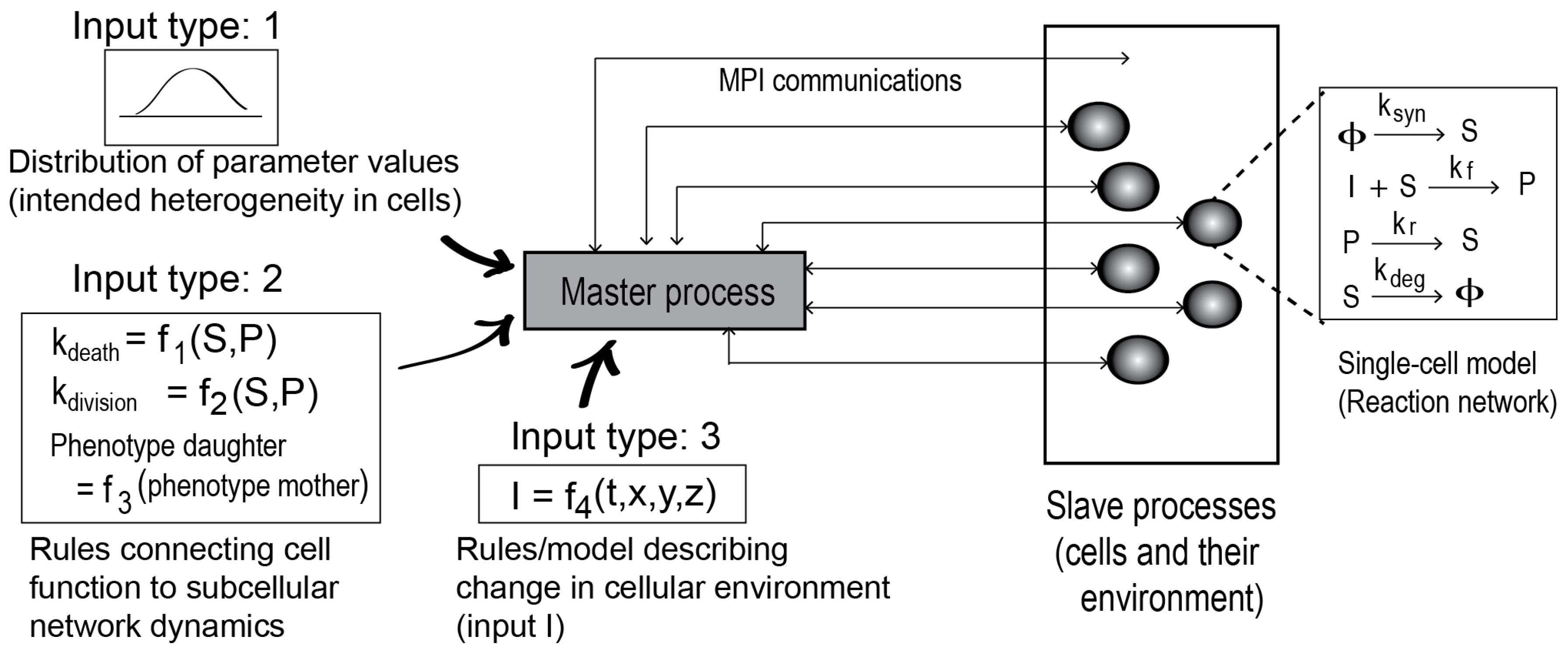
The biochemical network model could be a signaling pathway or gene transcription network model describing the intracellular protein-protein interaction and their biochemical transformations. The framework also requires three additional inputs, as shown. The Type 1 inputs are cellular distributions of the model parameter values and protein copy numbers. Distribution functions can be defined for the parameters and initial concentrations to incorporate cell-to-cell variability in the population model. The Type 2 inputs are model-specific rules that link the temporal intracellular events (time evolution of a network species, for example) to cellular functions (death, division, or phenotypes). The Type 3 inputs define the cell environment (growth condition).
Given the inputs, the framework launches parallel simulations on the single cell biochemical network model. Each of the simulation processes is then treated as a cell object, as in an agent-based model. Based on the parameter distribution functions, each cell object may acquire properties that are distinct from the other cell objects in the population.
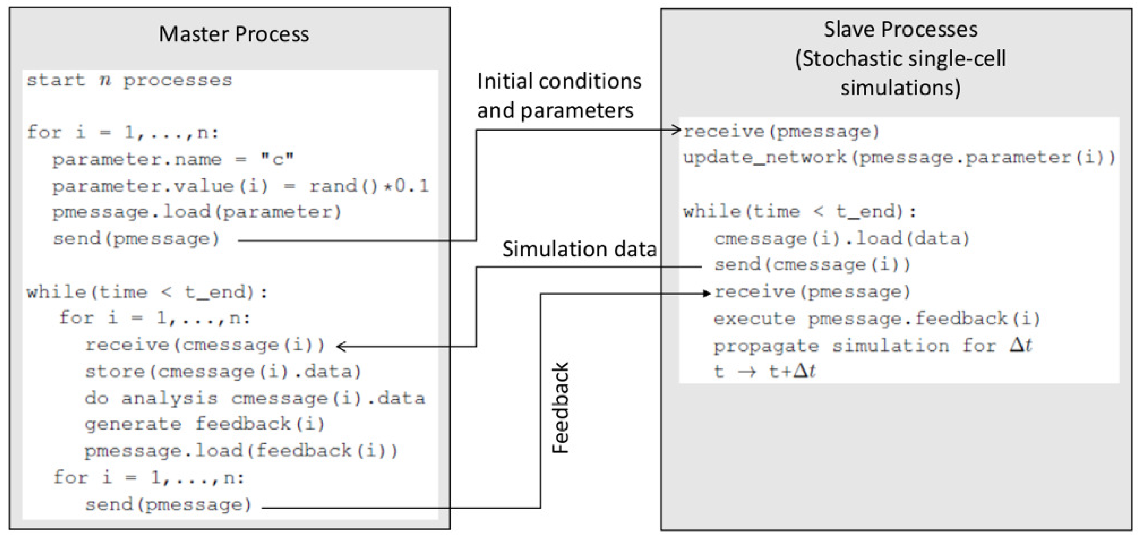
The framework works as a server (a master process), while each of the parallel simulations on the biochemical network model serves as a client (a slave process). MPI is used to mediate the server-client communications. A detailed algorithm of this server-client scheme is provided in Supplementary Materials (S1_File.pdf). This sever-client scheme is illustrated in Figure 2. Each cell object (slave process) is allowed to propagate simulation (Gillespie algorithm on the intracellular network) for a prescribed time interval . At the end of each , the master process and the slave processes communicate. The master process collects simulation data from each slave process (cell object) and analyzes the data against the rules (Type 2 and Type 3 inputs). Based on the analysis, it sends cell-specific instructions to each slave process using MPI. In addition, it takes actions to execute death, division, or other functions for a cell object if corresponding conditions specified in the rules are met.
If the internal state of any cell object meets the conditions for cell death (specified in the Type 2 rules), the master process terminates the parallel process. Similarly, if the internal state of a cell object meets the conditions for cell division, the master launches a new parallel process to create a daughter cell object. It then sends an MPI message to the newly created process to specify its initial condition, as defined in the rules (Type 2 inputs). Following cell division, the framework partitions the contents (network species) of the mother cell between the mother and the daughter based on binomial distribution [10].
Based on the Type 3 inputs, the master process evaluates the extracellular environment in each . It sends MPI messages to the cell objects about the updated environment variables. Such variables may include the concentration of an extracellular signal (the concentration of a drug, ligand, or other biomolecules, for example) that may affect the intracellular reactions. Based on the updated environment, the cell objects propagate simulation for another , and the process can be repeated.
It should be noted that the algorithm above is based on an approximation, rather than the accurate implementation of the Gillespie method. The approximation involves discretizing time in small intervals () within which the cells are assumed independent (simulated in parallel). An accurate implementation of the Gillespie algorithm over a multicellular system could be impractical if the detailed molecular interactions are considered at the single-cell level.
We discretize the simulation time with s. The assumption here is that the change in the extracellular environment in this period is small. In addition, this period is also small compared to the time scale of the cellular processes (death and division), which typically take several minutes to hours. This approximation may potentially improve computation, as we demonstrate in the result section. In our algorithm, the time step can be chosen arbitrarily small. However, a smaller could increase the frequency and overhead of the MPI communication.
2.2. Simple Models
Considering two simple intracellular networks, we demonstrate how the MPI framework builds population models by expanding a single-cell biochemical network model. These simple models are illustrated in Figure 3.
2.2.1. Model I
In this model, we consider cells as independent objects. Therefore, the death, division, or intracellular reactions of any cell is not affected by other cells in the population.
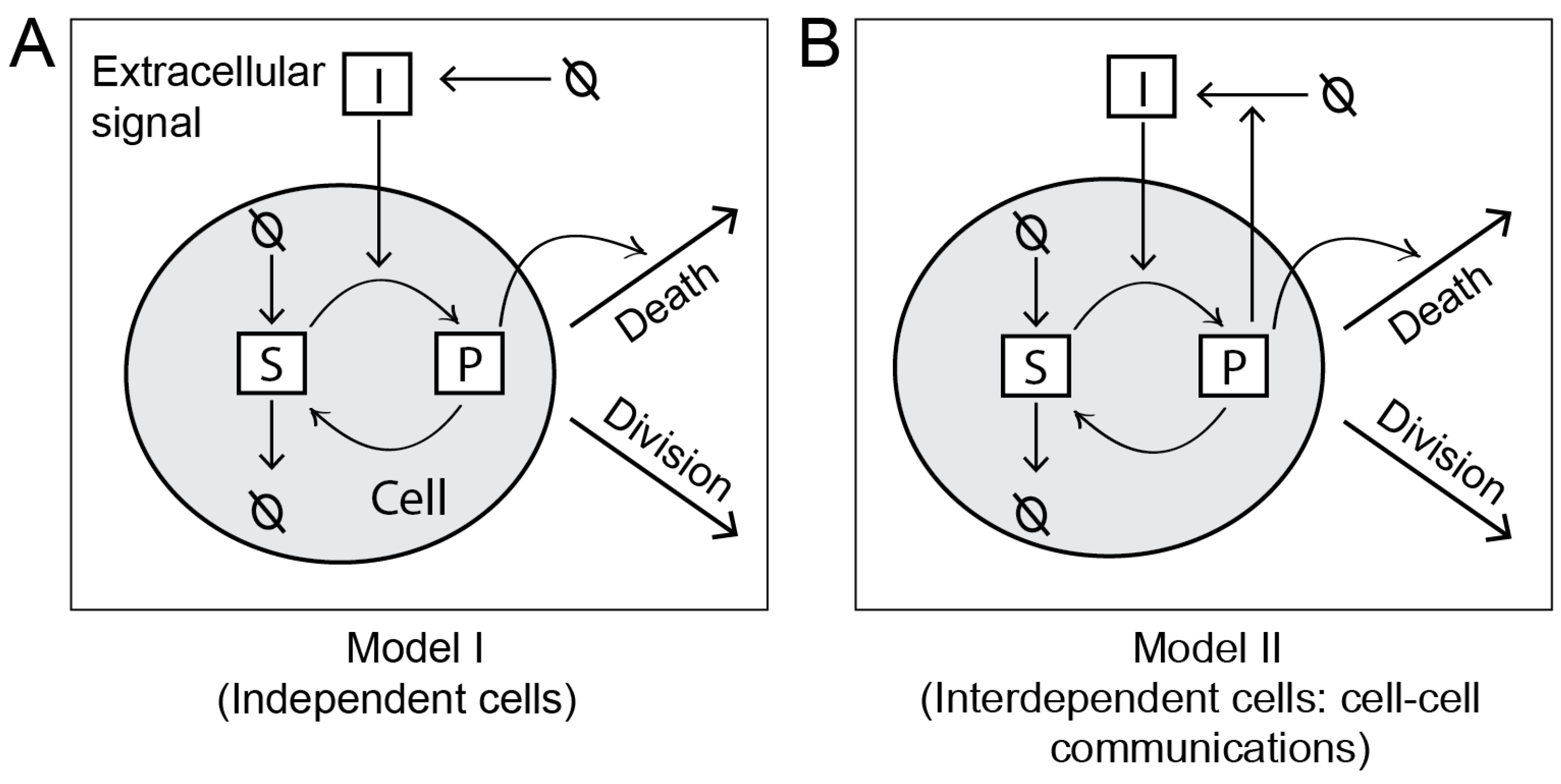
In a C++ program, we define a biochemical network model describing the intracellular events at the molecule scale. As illustrated in Figure 3A, we consider four elementary reactions in the network. These reactions and corresponding rate constants are listed in Table 1. The reactions describe a signaling pathway, which is activated in response to an extracellular signal I. A receptor protein S is synthesized and degraded in a zeroth and first-order reaction, respectively. In the presence of extracellular I, S is activated to produce P and deactivated in a reverse reaction. In the model, P serves as a pro-death signal for a cell. Intracellular accumulation of P elicits cell death by inducing the mean rate of cell death .
In a separate C++ program, we introduce the cellular processes and associated parameters (Table 2). We ignore cellular heterogeneity (Type 1 input). A rule (Type 2 input) is included to define the dependency of cell death on intracellular P. This rule simply states a linear relationship: (Table 2). Here, is the mean rate of cell death in the absence of P or extracellular I. The proportionality constant (Table 2) measures the sensitivity of a cell to intracellular P. A second rule is included to binomially distribute the contents (network species) of a cell when it is divided to create a new cell. We assume that the extracellular environment (I) remains unchanged throughout the simulation.
As explained earlier, we have two programs: one program (acting as slave) defining the biochemical network model, and the other program (acting as master) defining the cellular processes. These two programs contain complementary MPI calls to communicate in a server-client fashion. The master program launches a number of parallel simulations on the slave program to create the initial population of cell objects. For an interval, s, all the simulation processes (cell objects) propagate simulations (Gillespie algorithm) on the biochemical network system. At the end of , the master process collects simulation data from the cell objects. Based on the analysis of the simulation data against the rules, the master process performs few checks and takes actions accordingly. First, it evaluates each cell object for death or division. A cell is selected for death if , where is a uniform random number between 0 and 1. Similarly, a cell is selected for division if . Cell death is executed by terminating the corresponding parallel process, while cell division is executed by creating a new process (daughter cell) from the existing process (mother cell). The master process then analyzes the level of pro-death signal P in each (living) cell and updates the cell’s according to the rule. Note that cell death could be linked to a variety of pro-death (apoptotic) signals, such as an external cue [11,12,13] or intracellular expression of a death-inducing protein [14,15]. In this example model, P represents such an intracellular signal. The framework allows arbitrary functions (rules) linking such signals to cell death. The function, which is a modeler’s choice, could be defined based on an educated guess and existing knowledge.
While the master process performs the checks mentioned above, the slave processes (cell objects) remain in a blocking mode. This blocking mode is released upon receiving a message from the master program. The slave processes then propagate simulation for another , and the process is repeated until the simulation end time is reached.
2.2.2. Model II
This model is shown in Figure 3B. The model has the same set of intracellular reactions as Model I. However, in this model, cells are interdependent due to cell-to-cell communication. We consider a reaction whereby cells can secrete I in proportion to their intracellular P. Thus, each cell contributes to the global pool of I in the environment, which is shared by all cells. An increase in I in the environment further stimulates the intracellular production P in the cells, thus inducing cell death.
The slave program of Model II defining the biochemical network model remains essentially the same as in Model I, with the exception of the master program, where an additional rule (Type 3 input) is included. According to this rule, a cell i secretes amount of I in time : , where is a constant (Table 2) and is the intracellular P at time t. The total change of the environment is computed by summing up the contributions from all cells: , where is the number of cells at time t.
As in Model I, the master process communicates with the slave processes after each interval, s, and evaluates cell death, division, and for each of the cell objects. In addition, it also evaluates the change in I in the environment. It then updates the slave processes (cell objects) about the change in the environment by sending MPI messages. Upon receiving the MPI message, the cell object replaces the old I with a new I. Each cell object then propagates simulation for based on the new extracellular environment. The process is repeated until the simulation end time is reached.
2.2.3. Scalability and Performance Analysis
We first test our Model I for its computational performance. The test is performed against an equivalent model (referred to as sequential model), which is developed based on the traditional (non-parallel) formulation. In this sequential model, the intracellular reactions in all cells are gathered into a single reaction list. In addition, this list also contains the division and death of individual cells as reactions. The reactions in this list is then probabilistically sampled and executed by the exact Gillespie method.
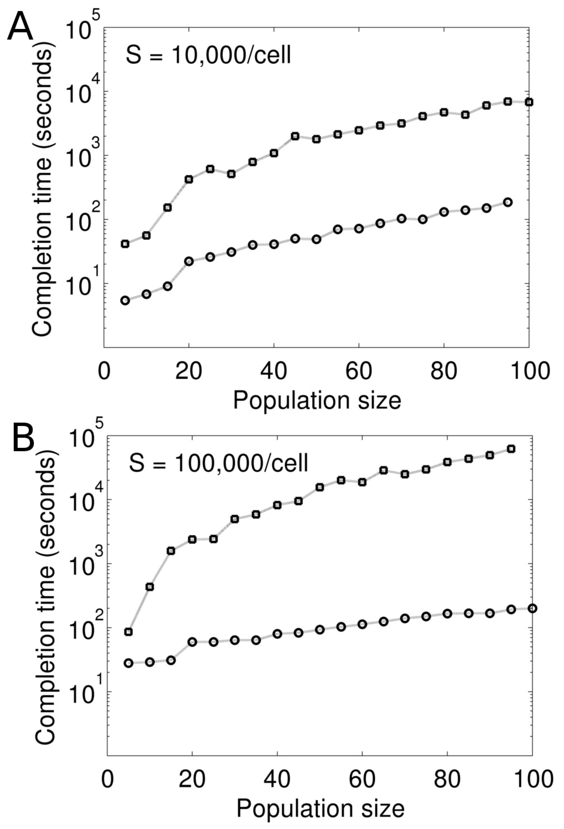
Figure 4 compares these two models in terms of their scalability and speed of computation. We vary the scale of the model by changing the cell population size. For consistency, all simulations are performed in the absence of stimulation (). This is to ensure that the mean cell population size remains constant during the simulations. For each population size, we simulate the two models for 1000 s and note the simulation completion time (wall clock seconds) (Figure 4). The simulations are carried out on a dedicated 20-core machine.
As seen in Figure 4, computation is orders of magnitude faster in the parallel formulation compared to its sequential counterpart. The difference becomes more significant when the models are made more computationally expensive by increasing the concentration of molecule S (Figure 4). Figure 4B represents a 10-fold higher S in the models compared to Figure 4A. Simulation using the Gillespie method at the cellular level becomes more expensive when S is increased. This makes computation prohibitively slow in the sequential model.
The faster computation in the parallel formulation is due to the MPI parallelism as well as the numerical approximation in the algorithm. As explained in the method section, we discretize the simulation time in s. In each , the cell objects are simulated independently and in parallel. At the end of each , the cell objects are synchronized and updated. On the contrary, in the sequential model, the Gillespie algorithm is accurately implemented over a single reaction list that represents the entire multicellular system. The sequential model is not scalable as the number of reactions in the list is determined by the number of cells in the system. In the parallel formulation, the time discretization ( s) is small because the mean waiting time for cell death and division is much longer ( s). We expect some loss of accuracy from this approximation, which, however, significantly improves computation.
Note that the concentrations and in the example above are arbitrarily chosen for the demonstration purpose. These numbers represent a typical expression level of many cellular signal transduction proteins [16]. However, the framework permits a model to incorporate a much larger protein copy number in the range of a few hundred thousands [17]. Its computation for a multicellular system remains feasible as long as the Gillespie algorithm at the single-cell remains tractable.
2.2.4. MPI to Link Intracellular Dynamics to Population Response
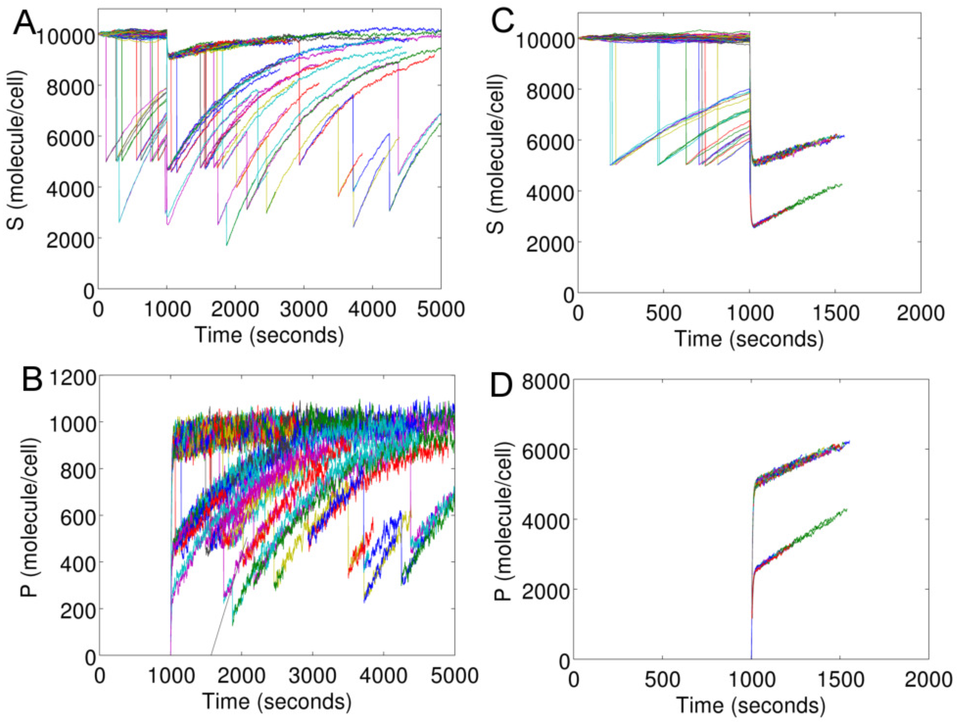
The rate of cell death in Model I is linked to the intracellular concentration of P (activated S) by a linear function, as discussed in the Method section. Figure 5 shows intracellular S and P of individual cells in an evolving cell population. We launch an initial population of 100 cells (parallel processes) at time zero. At s, the population is stimulated with s (Figure 5A,B) and s (Figure 5C,D).
In Figure 5, each curve for S or P represents an individual cell. The start and end of a curve correspond to the birth and death time of a cell, respectively. The sharp fall of any curve marks a cell division. The fall is due to the decrease in the cellular content of a mother cell because of its division. When a cell divides, the contents (network species) are divided between the two cells based on binomial distribution.
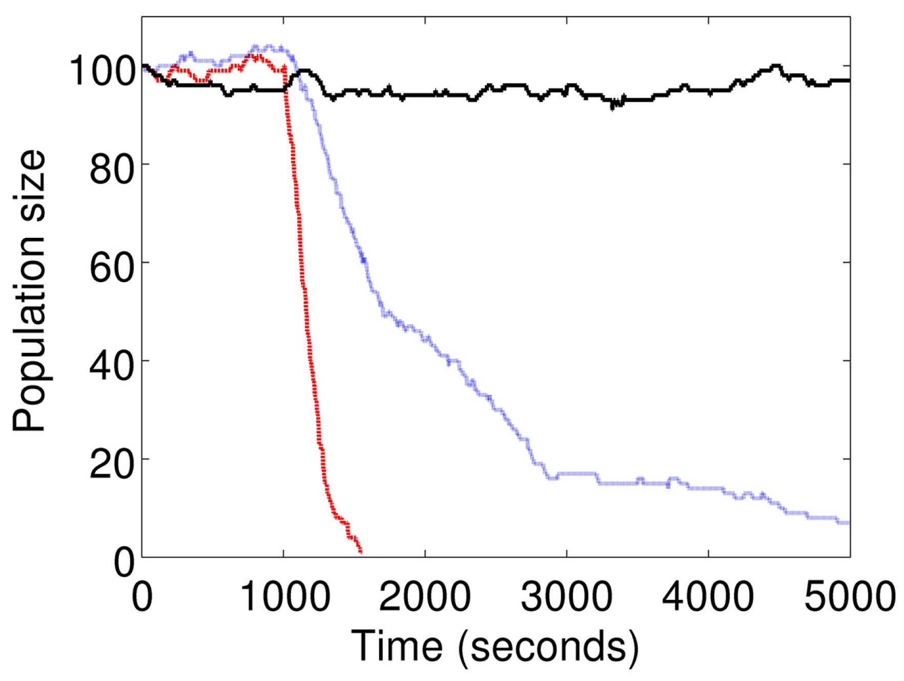
Figure 6 shows the cell population size at different doses of I. The curve showing a constant mean population size represents the basal condition (). The intermediate curve indicates a slow decline in the population size represents stimulation at s. The curve indicating a sharp decline represents stimulation at s.
2.2.5. MPI to Link the Intracellular Reactions and Cell Environment
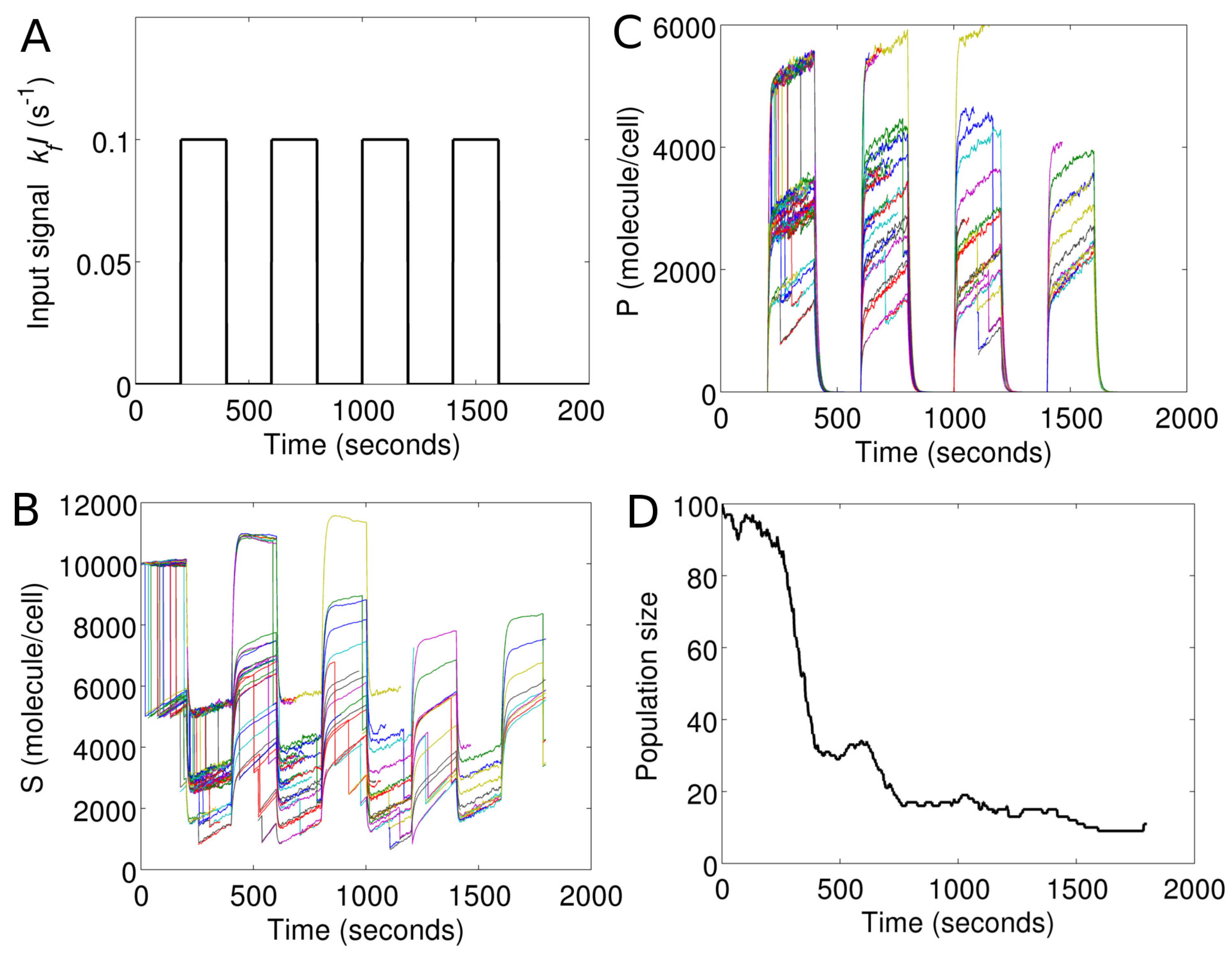
Figure 7 demonstrates cell population response in Model I under a temporally-evolving extracellular environment. To model the cell environment, we simply include an additional rule (Type 3 input) in the master program of Model I. This rule introduces a periodic pulse in I, as shown in Figure 7A.
At the end of each , the master program sends a message to each cell object. The message contains a new value of I for the global environment, which is shared by all cells. Upon receiving the message, the new value of I replaces the old one, in each cell object. The cell objects then propagate the reactions (Gillespie algorithm) based on this new value of I. Figure 7B,C show the intracellular S and P in each cell in the changing environment. Figure 7D shows corresponding changes in the cell population size as a function of time.
2.2.6. MPI to Model Cellular Communications
Our Model II is inspired by multicellular systems where cell-to-cell communications determine the collective behavior of cells [18]. In many physiologically-relevant systems, cells respond in an interdependent manner. Such dependencies may arise from the direct or indirect communications among the cells. Cells may directly communicate via physical interactions [19]. On the other hand, indirect communications may arise when cells modify a shared growth environment. Cells can release proteins or metabolites into the environment, which may affect other cells. An example of such indirect communication is called quorum sensing [20].
Recent studies have identified a family of quorum-sensing peptides, called Extracellular Death Factors (EDFs), that induces programmed cell death in E. coli [21] and several other bacteria [22]. Reportedly, secretion of these peptides by bacteria may elicit collective cell death in a population. In Model II, we consider a similar scenario where cells can produce and secrete I in proportion to their intracellular P. We implement this by simply adding a rule (a Type 3 input) in the master program of Model I. In each s, the master program evaluates the intracellular P in each cell object and the secretion of I by the cell object. The global environment is changed based on the contributions from all cells in the population. The change in the environment is implemented by sending MPI messages, as explained in the previous section.
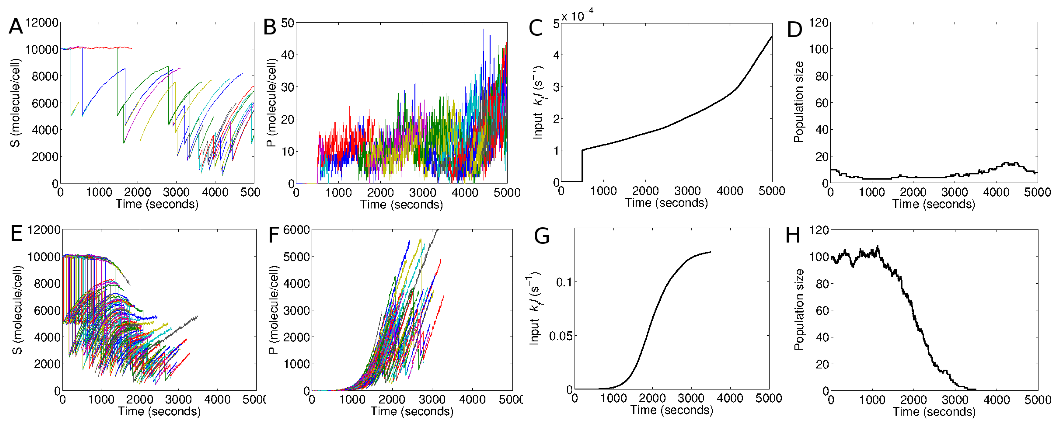
Figure 8 shows the population response in Model II. In the top panels (Figure 8A–D), an initial population of 10 cells are launched at time zero, and stimulated at s with a small dose of the extracellular signal, s. The population remains non-responsive to this signal. The average population size is not affected, as seen in Figure 8D. In the bottom panels (Figure 8E–H), an initial population of 100 cells are launched and subjected to the same level of stimulation, s, at s. Except for the population size, all other conditions are identical to those in the top panels. Nevertheless, contrary to the smaller population, this larger population displays a dramatic response (Figure 8E,F). The quorum-sensing positive feedback is triggered because of the collective contribution of the population. This leads to a rapid buildup of intracellular P (Figure 8F) and extracellular I (Figure 8G). As a result, the population shows a rapid post-stimulation decay (Figure 8H).
It should be noted that the selection of the population sizes in this example (100 or 10 cells) is completely arbitrary. In reality, millions of cells may participate in such a process. Nevertheless, the same qualitative differences could be reproduced at different relative scales of the model. An increase in the model scale (population size) would simply require an adjustment in the parameter (Table 2), which denotes the rate of secretion of I by each cell per molecule of its intracellular P.
3. A Full-Scale Model: Bacterial Quorum Sensing
Our previous examples involved two mock models with very simple sets of intracellular reactions. Here, we consider a full-scale model of bacterial quorum sensing with a more complex intracellular biochemical network. The model is based on an earlier model by Boada et al. [8]. The intracellular biochemical network reactions associated of this model are illustrated in Figure 9. The MPI expansion of this reaction network system into a population model is also illustrated in Figure 9.
In the master-slave scheme of our framework (Figure 9), the biochemical reactions in each cell is independently simulated using the Gillespie algorithm for a short interval . Each cell object simulates the Gillespie algorithm based on the reactions shown in Figure 9. The updated intracellular species concentrations from each cell object (slave process) are sent back to the master process using MPI. The master process then updates the common (well-mixed) extracellular environment based on the rules specified as an input to the master process (Figure 9). Here, the master takes two types of inputs. Type 1 input describes the distribution of parameters to incorporate cellular heterogeneity and type 2 input is the relationship between cell and environment defined as the net change between external autoinducer concentration () and internal autoinducer concentration (AHL) over each time interval . The parameters values associated with this model are taken from [8].
In the model, cell division is simulated by splitting the molecular concentration of the mother cell based on binomial distribution into two daughter cells. The cell population size is kept constant by killing (removing) a randomly selected cell (parallel thread) every time a cell division occurs.
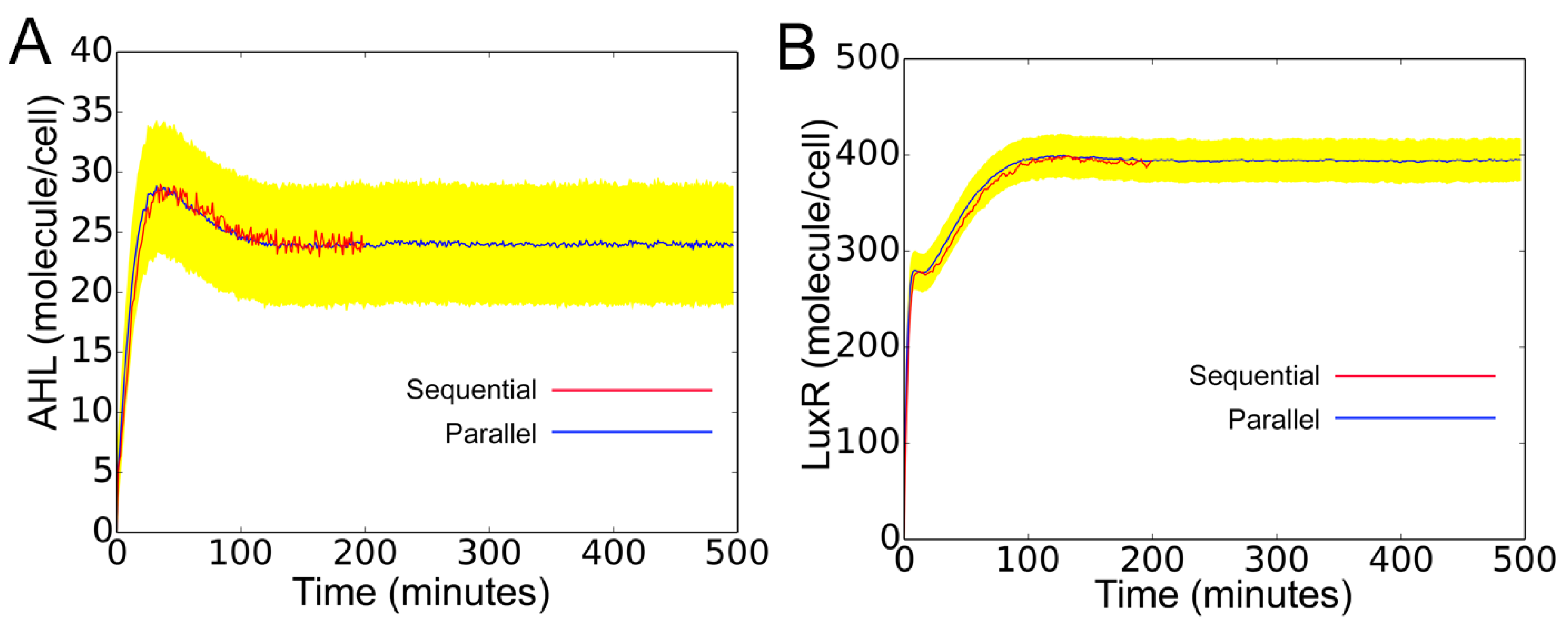
In Figure 10, we validate the above model against a corresponding accurate (sequential) model. In the sequential model, the intracellular reactions, cell death, and divisions associated with all cells in the population are grouped into one single list. The reactions from this list are sampled and executed following the Gillespie algorithm. As seen in the figure, despite the independent simulation of cells for discrete interval , the parallel model is in perfect agreement with the sequential model. The yellow region is the standard deviation, representing cell-to-cell variability arising from distribution of rate constant parameters. The change of molecular concentration under cellular birth and death are shown in Supplementary Materials (S2_File.pdf).
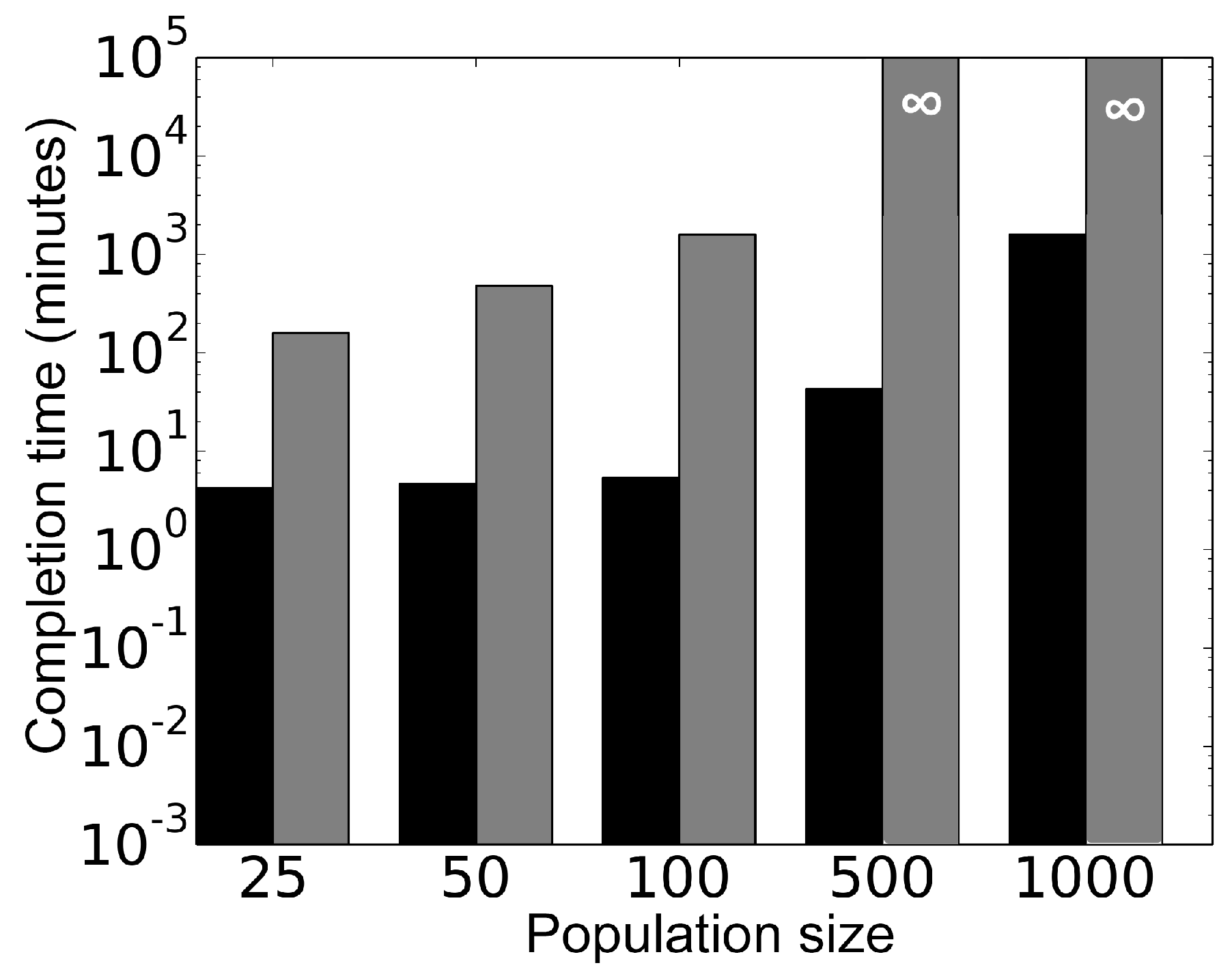
Figure 11 shows comparison of the computational performance between the parallel model and the sequential model, carried out on dedicated 50 cores of a high performance computing cluster. Using the two models, different cell population sizes were simulated for 100 min and corresponding simulation completion times (clock time) were recorded for each model. The result indicates the parallel algorithm is at least two orders of magnitude faster than the corresponding sequential algorithm for a population of 25 cells. Moreover, this gap between the parallel and the sequential algorithms widens with the increase in population size. Note that existing literature on quorum sensing [23,24] shows modeling of up to 240 cells using sequential approaches. Figure 11 shows that simulation of 500 and 1000 cells using the sequential approach remain unfinished after 168 h and are denoted by ∞. On the contrary, the proposed parallel framework exhibits scalability by simulating up to 1000 cells in less than 18 h.
4. Discussion
The goal of this work is to introduce a systematic method for developing mechanistic but computationally efficient cell population models. The question that we raise here is whether it is possible to systematically expand a biochemical network model into a cell population model. The commonly employed techniques to model multicellular systems include the continuum (equation-based) approach, cellular potts modeling (CPM) [25], and discrete agent-based modeling [26]. The equation-based approach and CPM are useful for modeling long-time behavior and evolution of cells. However, these methods have limited ability to capture the intracellular protein-protein interactions in a population model.
Arguably, agent-based modeling (ABM) is the most versatile framework for mechanistic modeling of multicellular systems [27,28,29,30]. In an agent-based model, individual cell agents could be assigned with cellular attributes at various time and spatial scales. However, mechanistic agent-based models could be computationally expensive and demand significant programming efforts.
Unlike the agent-based approach, we represent cells by stand-alone parallel simulation processes on a biochemical network model. We have shown that MPI-based remote communications can be used to treat such parallel processes as software objects like an agent-based model. In an agent-based approach, parallelism could also address the scalability issues and speed up computation. However, such implementation could be model-specific and require expertise in parallel logic implementation. We aim at providing a modular framework that would require minimal programming efforts. We separate a model into two different programs. We show that cellular-scale processes described in one program can be linked to the molecular-scale processes described in another program remotely to create a unified model. This allows a cellular and a biochemical network model to be defined separately and then combined to create a mechanistic population model.
Our framework is currently developed in an ad hoc approach that can only support biochemical network models written in C++ in a prescribed format. Nevertheless, the framework can be extended to make it compatible with other modeling languages and software platforms. It can be extended to create cell population models from the biochemical network models developed using other tools.
For demonstration purposes, the cellular protein-protein interactions in our example model is defined by a network of four elementary reactions. However, the network could be made as detailed as intended. Many advanced tools can develop highly mechanistic biochemical network models. For example, the rule-based modeling tools [31,32,33] can model biochemical network systems where cellular protein molecules can be defined with their site-specific details, such as binding domains and phosphorylation motifs [34,35,36]. Our framework can be integrated with such tools. This can be easily accomplished by embedding necessary MPI calls between a master program and the program running the simulation on a rule-based model. Such integration may provide the ability to study cellular evolution arising from the site-specific (point) mutations in the cellular protein domains and motifs.
This framework can only extend biochemical network models formulated in a stochastic approach, such as the Gillespie method [9]. In a stochastic model, it is possible to introduce a run-time change in the model parameter values and simulation conditions. In a deterministic model, such changes would lead to discontinuities. Therefore, it is not extensible for the deterministic models.
An important limitation of our approach is that it must synchronize the parallel simulation processes (cell objects) at discrete intervals. The synchronization limits the computation speed by the slowest process in a population. In a large number of parallel processes implementing stochastic simulations, the cost of computation could be considerably different from the processes. This issue could be partially addressed by developing a dynamic load-balancing and resource allocation scheme.
A second limitation is an overhead associated with MPI communications. For a large number of cells in a model, such communication overhead could be significant. Overhead can be the limiting factor if the simulation of the biochemical network is not computation intensive. This issue could be partly addressed through serialization of the MPI messages. In the current framework, the messages are passed as C data structures without serialization. The cost of overhead could also be addressed by developing a more distributed system having multiple servers and clients. Our current framework is based on a centralized system, where communications occur between a single server and multiple clients.
We have applied our framework to model quorum sensing in bacteria, where we consider a homogeneous distribution of environment across all cells and their interaction with the environment through diffusion. As part of future work, we shall extend it to accommodate spatial position of cells and the environmental molecules as discussed in [37,38] to incorporate the cellular heterogeneity. There would be a minor variation in our framework once the spatial model is incorporated. At present, our framework constitutes a master module which controls the activities of the cells in the system. In the spatial model, our master node will re-determine the coordinates of the cells and environmental molecules after fixed intervals of time.
This framework can be extended to model other bacteria, yeast [39], fungus and higher organisms (eukaryotic cells) [40,41]. For example, different proteins that copy number of yeast and Hela cells are listed in Kulak et al. [16]. These modelings will follow a similar approach as quorum sensing, where bacteria synchronize themselves based on feedback response from their environment.
Our framework presents a general approach to connect the molecular scale to the cell population scale. It is noteworthy that cancer cells have similar multi scale features in low scale (production of molecules from genes), intermediate scale (interaction of gene with its cellular environment) and high scale (collective behavior of cells) [42,43,44,45]. Our framework can incorporate these hallmarks to study the nature and phenotype of cancer cells. Furthermore, we intuit that our proposed framework can also be applied to any drug delivery system, where the concentration of optimum drug dosage can be quantitatively estimated [11,12,13,46]. The different dosages (e.g., constant dose, periodic dose) of drugs can be modeled as environmental variables as described in Figure 6 and Figure 7.
Finally, our approach could also find applications in modeling biological systems that are of scientific, pathological, and clinical interests. Examples include the evolutionary mechanisms of stem cells [47], clonal expansion of B and T lymphocytes [48,49], autocrine, paracrine, and endocrine signaling [50,51], and chemotactic cell migration [52].
5. Conclusions
In this work, we demonstrate a new framework for systematic development of multiscale cell population models. The framework takes a biochemical network model as an input and expands it into a population model by linking intracellular network dynamics to cellular functions, fate decisions, and evolution. This capability is provided by a unique message passing interface (MPI) scheme. The MPI scheme also enables modeling cell-to-cell and cell-environment communications. The framework is further extensible to modeling multicellular systems evolving under both spatially- and temporally-resolved growth environments.
Supplementary Materials
The following files are available online at https://www.mdpi.com/2227-9717/6/11/217/s1, File S1_File.pdf describes the simulation algorithm of the MPI framework. File S2_File.pdf describes molecular concretration over time under cellular birth and death in Quorum Sensing.
Author Contributions
Conceptualization, D.B.; Software Code, M.A.I., S.R. and D.B.; Formal Analysis, M.A.I., S.R. and D.B.; Investigation, M.A.I., S.R., D.B.; Resources, D.B. and S.K.D.; Data Curation, M.A.I. and S.R.; Writing—Original Draft Preparation, D.B.; Writing—Review and Editing, D.B., S.K.D., M.A.I. and S.R.; Supervision, D.B. and S.K.D.; Project Administration, D.B. and S.K.D.; Funding Acquisition, D.B. and S.K.D.
Funding
This research was funded in part by the National Science Foundation (Award No. CBET-CDS&E 1609642), and the University of Missouri Research Board (UMRB).
Conflicts of Interest
The authors declare no conflict of interest.
Abbreviations
The following abbreviation is used in this manuscript:
| MPI | Message Passing Interface |
References
- Moignard, V.; Göttgens, B. Transcriptional mechanisms of cell fate decisions revealed by single cell expression profiling. Bioessays 2014, 36, 419–426. [Google Scholar] [CrossRef] [PubMed] [Green Version]
- Fazi, F.; Nervi, C. MicroRNA: Basic mechanisms and transcriptional regulatory networks for cell fate determination. Cardiovasc. Res. 2008, 79, 553–561. [Google Scholar] [CrossRef] [PubMed]
- Xiong, W.; Ferrell, J.E. A positive-feedback-based bistable ‘memory module’ that governs a cell fate decision. Nature 2003, 426, 460–465. [Google Scholar] [CrossRef] [PubMed]
- Qu, Z.; Garfinkel, A.; Weiss, J.N.; Nivala, M. Multi-scale modeling in biology: How to bridge the gaps between scales? Prog. Biophys. Mol. Biol. 2011, 107, 21–31. [Google Scholar] [CrossRef] [PubMed] [Green Version]
- Meier-Schellersheim, M.; Fraser, I.D.; Klauschen, F. Multiscale modeling for biologists. Wiley Interdiscip. Rev. Syst. Biol. Med. 2009, 1, 4–14. [Google Scholar] [CrossRef] [PubMed]
- Gropp, W.; Lusk, E.; Skjellum, A. Using MPI: Portable Parallel Programming with the Message-Passing Interface; MIT Press: Cambridge, MA, USA, 1999; Volume 1. [Google Scholar]
- Gilbert, N. Agent-Based Models; Number 153; Sage: Thousand Oaks, CA, USA, 2008. [Google Scholar]
- Boada, Y.; Vignoni, A.; Pico, J. Promoter and transcription factor dynamics tune protein mean and noise strength in a quorum sensing-based feedback synthetic circuit. bioRxiv 2017, 106229. [Google Scholar] [CrossRef] [Green Version]
- Gillespie, D.T. A general method for numerically simulating the stochastic time evolution of coupled chemical reactions. J. Comput. Phys. 1976, 22, 403–434. [Google Scholar] [CrossRef]
- Soltani, M.; Singh, A. Effects of cell-cycle-dependent expression on random fluctuations in protein levels. R. Soc. Open Sci. 2016, 3, 160578. [Google Scholar] [CrossRef] [PubMed] [Green Version]
- Pujol, J.M.; Eisenberg, J.E.; Haas, C.N.; Koopman, J.S. The effect of ongoing exposure dynamics in dose response relationships. PLoS Comput. Biol. 2009, 5, e1000399. [Google Scholar] [CrossRef] [PubMed]
- Venkatratnam, A.; House, J.S.; Konganti, K.; McKenney, C.; Threadgill, D.W.; Chiu, W.A.; Aylor, D.L.; Wright, F.A.; Rusyn, I. Population-based dose–response analysis of liver transcriptional response to trichloroethylene in mouse. Mamm. Genome 2018, 29, 168–181. [Google Scholar] [CrossRef] [PubMed]
- Gu, J.; Zhang, X.; Ma, Y.; Li, N.; Luo, F.; Cao, L.; Wang, Z.; Yuan, G.; Chen, L.; Xiao, W.; et al. Quantitative modeling of dose–response and drug combination based on pathway network. J. Cheminform. 2015, 7, 19. [Google Scholar] [CrossRef] [PubMed]
- Tan, X.H.; Song, Z.B.; Wang, H.; Wang, Q.; He, J.L. Influence of adjuvant levetiracetam therapy on serum nerve cytokines and apoptosis molecules in patients with refractory partial epileptic seizure. J. Hainan Med. Univ. 2017, 23, 145–149. [Google Scholar]
- Carpineto, P.; Aharrh-Gnama, A.; Ciciarelli, V.; Borrelli, E.; Petti, F.; Aloia, R.; Lamolinara, A.; Di Nicola, M.; Mastropasqua, L. Subretinal Fluid Levels of Signal-Transduction Proteins and Apoptosis Molecules in Macula-Off Retinal Detachment Undergoing Scleral Buckle Surgery. Investig. Ophthalmol. Vis. Sci. 2016, 57, 6895–6901. [Google Scholar] [CrossRef] [PubMed]
- Kulak, N.A.; Pichler, G.; Paron, I.; Nagaraj, N.; Mann, M. Minimal, encapsulated proteomic-sample processing applied to copy-number estimation in eukaryotic cells. Nat. Methods 2014, 11, 319–324. [Google Scholar] [CrossRef] [PubMed]
- Faeder, J.R.; Hlavacek, W.S.; Reischl, I.; Blinov, M.L.; Metzger, H.; Redondo, A.; Wofsy, C.; Goldstein, B. Investigation of early events in FcεRI-mediated signaling using a detailed mathematical model. J. Immunol. 2003, 170, 3769–3781. [Google Scholar] [CrossRef] [PubMed]
- De Mello, W.C. Cell-to-Cell Communication; Springer: New York, NY, USA, 2012. [Google Scholar]
- Hervé, J.C.; Derangeon, M. Gap-junction-mediated cell-to-cell communication. Cell Tissue Res. 2013, 352, 21–31. [Google Scholar] [CrossRef] [PubMed]
- Waters, C.M.; Bassler, B.L. Quorum sensing: Cell-to-cell communication in bacteria. Annu. Rev. Cell Dev. Biol. 2005, 21, 319–346. [Google Scholar] [CrossRef] [PubMed]
- Kolodkin-Gal, I.; Hazan, R.; Gaathon, A.; Carmeli, S.; Engelberg-Kulka, H. A linear pentapeptide is a quorum-sensing factor required for mazEF-mediated cell death in Escherichia coli. Science 2007, 318, 652–655. [Google Scholar] [CrossRef] [PubMed]
- Kumar, S.; Engelberg-Kulka, H. Quorum sensing peptides mediating interspecies bacterial cell death as a novel class of antimicrobial agents. Curr. Opin. Microbiol. 2014, 21, 22–27. [Google Scholar] [CrossRef] [PubMed]
- Weber, M.; Buceta, J. Dynamics of the quorum sensing switch: Stochastic and non-stationary effects. BMC Syst. Biol. 2013, 7, 6. [Google Scholar] [CrossRef] [PubMed]
- Boada, Y.; Vignoni, A.; Navarro, J.; Picó, J. Improvement of a cle stochastic simulation of gene synthetic network with quorum sensing and feedback in a cell population. In Proceedings of the 2015 IEEE European Control Conference (ECC), Linz, Austria, 15–17 July 2015; pp. 2274–2279. [Google Scholar]
- Graner, F.; Glazier, J.A. Simulation of biological cell sorting using a two-dimensional extended Potts model. Phys. Rev. Lett. 1992, 69, 2013–2016. [Google Scholar] [CrossRef] [PubMed]
- Jessica, S.Y.; Bagheri, N. Multi-class and multi-scale models of complex biological phenomena. Curr. Opin. Biotechnol. 2016, 39, 167–173. [Google Scholar]
- Bonabeau, E. Agent-based modeling: Methods and techniques for simulating human systems. Proc. Natl. Acad. Sci. USA 2002, 99, 7280–7287. [Google Scholar] [CrossRef] [PubMed] [Green Version]
- An, G.; Mi, Q.; Dutta-Moscato, J.; Vodovotz, Y. Agent-based models in translational systems biology. Wiley Interdiscip. Rev. Syst. Biol. Med. 2009, 1, 159–171. [Google Scholar] [CrossRef] [PubMed] [Green Version]
- Olsen, M.M.; Siegelmann, H.T. Multiscale agent-based model of tumor angiogenesis. Procedia Comput. Sci. 2013, 18, 1016–1025. [Google Scholar] [CrossRef]
- Zhang, L.; Wang, Z.; Sagotsky, J.A.; Deisboeck, T.S. Multiscale agent-based cancer modeling. J. Math. Biol. 2009, 58, 545–559. [Google Scholar] [CrossRef] [PubMed]
- Danos, V.; Feret, J.; Fontana, W.; Harmer, R.; Krivine, J. Rule-based modelling of cellular signalling. In CONCUR 2007–Concurrency Theory; Springer: Berlin/Heidelberg, Germany, 2007; pp. 17–41. [Google Scholar]
- Faeder, J.R.; Blinov, M.L.; Hlavacek, W.S. Rule-based modeling of biochemical systems with BioNetGen. In Systems Biology; Springer: New York, NY, USA, 2009; pp. 113–167. [Google Scholar]
- Sneddon, M.W.; Faeder, J.R.; Emonet, T. Efficient modeling, simulation and coarse-graining of biological complexity with NFsim. Nat. Methods 2011, 8, 177–183. [Google Scholar] [CrossRef] [PubMed]
- Barua, D.; Hlavacek, W.S.; Lipniacki, T. A computational model for early events in B cell antigen receptor signaling: Analysis of the roles of Lyn and Fyn. J. Immunol. 2012, 189, 646–658. [Google Scholar] [CrossRef] [PubMed]
- Barua, D.; Hlavacek, W.S. Modeling the effect of APC truncation on destruction complex function in colorectal cancer cells. PLoS Comput. Biol. 2013, 9, e1003217. [Google Scholar] [CrossRef] [PubMed]
- Creamer, M.S.; Stites, E.C.; Aziz, M.; Cahill, J.A.; Tan, C.W.; Berens, M.E.; Han, H.; Bussey, K.J.; Von Hoff, D.D.; Hlavacek, W.S.; et al. Specification, annotation, visualization and simulation of a large rule-based model for ERBB receptor signaling. BMC Syst. Biol. 2012, 6, 107. [Google Scholar] [CrossRef] [PubMed]
- Erban, R.; Chapman, S.J. Stochastic modelling of reaction–diffusion processes: Algorithms for bimolecular reactions. Phys. Biol. 2009, 6, 046001. [Google Scholar] [CrossRef] [PubMed]
- Resat, H.; Costa, M.N.; Shankaran, H. Spatial aspects in biological system simulations. In Methods in Enzymology; Elsevier: Amsterdam, The Netherlands, 2011; Volume 487, pp. 485–511. [Google Scholar]
- Ahn, T.H.; Wang, P.; Watson, L.T.; Cao, Y.; Shaffer, C.A.; Baumann, W.T. Stochastic cell cycle modeling for budding yeast. In Proceedings of the 2009 Spring Simulation Multiconference, Society for Computer Simulation International, San Diego, CA, USA, 22–27 March 2009; p. 113. [Google Scholar]
- Komalapriya, C.; Kaloriti, D.; Tillmann, A.T.; Yin, Z.; Herrero-de Dios, C.; Jacobsen, M.D.; Belmonte, R.C.; Cameron, G.; Haynes, K.; Grebogi, C.; et al. Integrative model of oxidative stress adaptation in the fungal pathogen Candida albicans. PLoS ONE 2015, 10, e0137750. [Google Scholar] [CrossRef] [PubMed] [Green Version]
- Clement, E.J.; Wysocki, B.J.; Soliman, G.A.; Wysocki, T.A.; Davis, P.H. Dynamic Modeling and Stochastic Simulation of Metabolic Networks. bioRxiv 2018, 336677. [Google Scholar] [CrossRef] [Green Version]
- Bellouquid, A.; De Angelis, E.; Knopoff, D. From the modeling of the immune hallmarks of cancer to a black swan in biology. Math. Models Methods Appl. Sci. 2013, 23, 949–978. [Google Scholar] [CrossRef]
- Zou, Y.; Laubichler, M.D. From systems to biology: A computational analysis of the research articles on systems biology from 1992 to 2013. PLoS ONE 2018, 13, e0200929. [Google Scholar] [CrossRef] [PubMed]
- Hanahan, D.; Weinberg, R.A. Hallmarks of cancer: The next generation. Cell 2011, 144, 646–674. [Google Scholar] [CrossRef] [PubMed]
- Bellomo, N.; Carbonaro, B. Toward a mathematical theory of living systems focusing on developmental biology and evolution: A review and perspectives. Phys. Life Rev. 2011, 8, 1–18. [Google Scholar] [CrossRef] [PubMed]
- Levchenko, A.; Nemenman, I. Cellular noise and information transmission. Curr. Opin. Biotechnol. 2014, 28, 156–164. [Google Scholar] [CrossRef] [PubMed] [Green Version]
- Humphries, A.; Cereser, B.; Gay, L.J.; Miller, D.S.; Das, B.; Gutteridge, A.; Elia, G.; Nye, E.; Jeffery, R.; Poulsom, R.; et al. Lineage tracing reveals multipotent stem cells maintain human adenomas and the pattern of clonal expansion in tumor evolution. Proc. Natl. Acad. Sci. USA 2013, 110, E2490–E2499. [Google Scholar] [CrossRef] [PubMed] [Green Version]
- Abbas, A.K.; Lichtman, A.H.; Pillai, S. Basic Immunology: Functions and Disorders of the Immune System; Elsevier: Amsterdam, The Netherlands, 2014. [Google Scholar]
- Qi, Q.; Liu, Y.; Cheng, Y.; Glanville, J.; Zhang, D.; Lee, J.Y.; Olshen, R.A.; Weyand, C.M.; Boyd, S.D.; Goronzy, J.J. Diversity and clonal selection in the human T-cell repertoire. Proc. Natl. Acad. Sci. USA 2014, 111, 13139–13144. [Google Scholar] [CrossRef] [PubMed] [Green Version]
- Singh, A.B.; Harris, R.C. Autocrine, paracrine and juxtacrine signaling by EGFR ligands. Cell Signal. 2005, 17, 1183–1193. [Google Scholar] [CrossRef] [PubMed]
- Ratajczak, M.Z.; Schneider, G.; Ratajczak, J. Paracrine Effects of Fetal Stem Cells. In Fetal Stem Cells in Regenerative Medicine; Springer: New York, NY, USA, 2016; pp. 47–56. [Google Scholar]
- Rappel, W.J. Cell–cell communication during collective migration. Proc. Natl. Acad. Sci. USA 2016, 113, 1471–1473. [Google Scholar] [CrossRef] [PubMed] [Green Version]
Figure 1.
Schematic diagram of the population modeling framework. The framework uses MPI parallelism to create a multiscale population model from a single-cell biochemical reaction network model. Each single cell is represented by a stand-alone parallel process. Intercellular communication is mediated in a server-client fashion. On the far right of the figure, an example set of biochemical network reactions associated with each cell is shown. The network consists of two intracellular species S and P and their synthesis, degradation, and inter-conversion in response to an extracellular cue I. The master process creates a population of cells, where each cell has this same set of biochemical reactions. However, the master process incorporates heterogeneity among the cells by sampling the protein copy number or parameter values from defined distributions (Input 1). In addition, the master process implements rules for cellular decision-making based on the intracellular species concentrations (Input 2). The master process also determines how the extracellular input I may change over time (t) or position () based on some defined rules (Input 3).

Figure 2.
The skeleton algorithm of MPI communications. The master program and the slave program are shown in the left and right box, respectively. The master program defines parameters and rules associated with the cellular-scale processes and extracellular environment. The slave program defines the molecular-scale processes in the form of a stand-alone biochemical network model. The master and slave programs contain complementary MPI calls in a loop to mediate communications in a server-client fashion.

Figure 3.
The two example (mock) models. The gray circle represents a cell, and the white space around the circle represents the extracellular space. The intracellular network consists of two species S and P. S is synthesized and degraded at a certain rate. In addition, it is converted into P in the presence of an extracellular species I. (A) Model I: cells are independent; (B) Model II: cells communicate by modifying the extracellular environment (concentration of I).

Figure 4.
Computational performance of Model I. Model I (circles) and its equivalent sequential model (squares) are simulated for 1000 s. The two panels correspond to different initial concentration of molecule S in the model, as shown. The x-axis represents the average cell population size in a simulation. The y-axis represents corresponding simulation completion time (clock seconds). Simulations are performed in a dedicated 20-core machine.

Figure 5.
Temporal evolution of S and P in individual cells. (A,B) the population is stimulated at s with ; (C,D) the population is stimulated at s with .
Figure 5.
Temporal evolution of S and P in individual cells. (A,B) the population is stimulated at s with ; (C,D) the population is stimulated at s with .

Figure 6.
Cell population dynamics at different doses of stimulation, indicated by black ( s), blue ( s), and red ( s), respectively.
Figure 6.
Cell population dynamics at different doses of stimulation, indicated by black ( s), blue ( s), and red ( s), respectively.

Figure 7.
Modeling cell environment using MPI. (A) the cell environment with pulse variation in extracellular I; (B) intracellular S of individual cells; (C) intracellular P of individual cells; (D) time evolution of the cell population size.
Figure 7.
Modeling cell environment using MPI. (A) the cell environment with pulse variation in extracellular I; (B) intracellular S of individual cells; (C) intracellular P of individual cells; (D) time evolution of the cell population size.

Figure 8.
Population response under cellular communications in Model II. In the top panels (A–D), an initial population of 10 cells was subject to s at s. In the bottom panels (E,F), an initial population of 100 cells is subject to s at s; (A,E) intracellular S in individual cells; (B,F) intracellular P in individual cells; (C,G) temporal evolution of extracellular I in the environment; (D,H) cell population size as function of time.

Figure 9.
Schematic diagram of the multicellular quorum sensing model. The master process expands the single-cell biochemical network (set of reactions shown) into a multicellular model. Type 1 input defines the distributions of the model/network parameters values to incorporate cellular heterogeneity. Type 2 input defines relationship between a cell and the extracellular environment defined as the net change between external autoinducer concentration () and internal autoinducer concentration (AHL) over each time interval .

Figure 10.
Prediction accuracy of the framework-created quorum sensing model is validated against an equivalent sequential model. Temporal evolution of (A) and (B) LuxR. The blue and red curves represent the parallel model and the sequential model, respectively. The yellow region is the standard deviation, representing cell-to-cell variability arising from distribution of parameters. The temporal profiles of these concentrations are similar to those shown in [8]. Note that the sequential model was run only up to 200 s due to the prohibitively slow computation.

Figure 11.
Semi-log plot for computational performance of the parallel quorum sensing model compared against a corresponding accurate (sequential) model. The black and grey bars represent the parallel and the sequential model, respectively. The infinite signs represent the cases where simulation of the sequential model remained unfinished after 168 h of simulation.


Table 1.
Signaling pathway model parameters (slave program).
| Parameter | Value | Description |
|---|---|---|
| S | 10,000 molecule/cell | Initial concentration of S. |
| P | 0 molecule/cell | Initial concentration of P. |
| I | (Varied) molecule/cell | Extracellular signal. |
| 10 molecules s | Rate constant for → S. | |
| 0.001 s | Rate constant for | |
| (molecule/cell)s | Rate constant for P. | |
| 0.1 s | Rate constant for . |
Table 2.
Cellular model parameters (master program).
| Parameter | Value | Description |
|---|---|---|
| s | Mean rate of cell death in the basal state. | |
| s | Mean rate of cell division. | |
| (molecule)s | Cell death sensitivity to intracellular P. | |
| s | Mean rate of cell death (function of intracellular P). | |
| (molecule)s | Model II only: rate of cellular production | |
| and release I per of molecule of intracellular P. |
© 2018 by the authors. Licensee MDPI, Basel, Switzerland. This article is an open access article distributed under the terms and conditions of the Creative Commons Attribution (CC BY) license (http://creativecommons.org/licenses/by/4.0/).
Share and Cite
MDPI and ACS Style
Islam, M.A.; Roy, S.; Das, S.K.; Barua, D. Multicellular Models Bridging Intracellular Signaling and Gene Transcription to Population Dynamics. Processes 2018, 6, 217. https://doi.org/10.3390/pr6110217
AMA Style
Islam MA, Roy S, Das SK, Barua D. Multicellular Models Bridging Intracellular Signaling and Gene Transcription to Population Dynamics. Processes. 2018; 6(11):217. https://doi.org/10.3390/pr6110217
Chicago/Turabian StyleIslam, Mohammad Aminul, Satyaki Roy, Sajal K. Das, and Dipak Barua. 2018. "Multicellular Models Bridging Intracellular Signaling and Gene Transcription to Population Dynamics" Processes 6, no. 11: 217. https://doi.org/10.3390/pr6110217
Note that from the first issue of 2016, this journal uses article numbers instead of page numbers. See further details here.