Elucidating Cellular Population Dynamics by Molecular Density Function Perturbations


1
Sage Bionetworks, Seattle, WA 98109, USA
2
Institute for Chemical and Bioengineering, ETH Zurich, Zurich 8093, Switzerland
3
Swiss Institute of Bioinformatics, Lausanne 1015, Switzerland
*
Author to whom correspondence should be addressed.
Processes 2018, 6(2), 9; https://doi.org/10.3390/pr6020009
Submission received: 21 December 2017
/
Revised: 16 January 2018
/
Accepted: 18 January 2018
/
Published: 23 January 2018
(This article belongs to the Special Issue Biological Networks)
Abstract
:Studies performed at single-cell resolution have demonstrated the physiological significance of cell-to-cell variability. Various types of mathematical models and systems analyses of biological networks have further been used to gain a better understanding of the sources and regulatory mechanisms of such variability. In this work, we present a novel sensitivity analysis method, called molecular density function perturbation (MDFP), for the dynamical analysis of cellular heterogeneity. The proposed analysis is based on introducing perturbations to the density or distribution function of the cellular state variables at specific time points, and quantifying how such perturbations affect the state distribution at later time points. We applied the MDFP analysis to a model of a signal transduction pathway involving TRAIL (tumor necrosis factor-related apoptosis-inducing ligand)-induced apoptosis in HeLa cells. The MDFP analysis shows that caspase-8 activation regulates the timing of the switch-like increase of cPARP (cleaved poly(ADP-ribose) polymerase), an indicator of apoptosis. Meanwhile, the cell-to-cell variability in the commitment to apoptosis depends on mitochondrial outer membrane permeabilization (MOMP) and events following MOMP, including the release of Smac (second mitochondria-derived activator of caspases) and cytochrome c from mitochondria, the inhibition of XIAP (X-linked inhibitor of apoptosis) by Smac, and the formation of the apoptosome.
1. Introduction
Advances in single-cell profiling technology and the application of this technology to study biology at single-cell resolution have demonstrated the ubiquity and functional role of cell-to-cell variability in physiological processes, such as programmed cell death (apoptosis) and stem cell differentiation [1,2,3]. Besides genetic, epigenetic, and environmental factors, the cellular heterogeneity observed in a given cell population has also been attributed to the inherent stochastic dynamics of cellular processes. For example, gene transcriptional processes have been shown to occur in stochastic (random) bursts [4,5,6]. Many modeling frameworks have been used to capture cellular heterogeneity—for example, by using ensemble models (EM) of ordinary differential equations (ODEs) [7,8,9], population balance models (PBMs) [10], stochastic ordinary differential equations (SDEs) [11,12], and chemical master equations (CMEs) [13,14,15]. In these models, the cell-to-cell variability is described by a probability density or distribution function of cell state variables. Systems analyses have also been developed and applied to gain insight into the dynamics of cell state distribution. For example, several types of parameter sensitivity analysis, including SOBOL sensitivity [16], derivative-based global sensitivity measure (DGSM) [17], glocal analysis [18], extended Fourier amplitude sensitivity test (eFAST) [19], and stochastic sensitivity analysis [20,21,22,23] have been used to identify the rate-controlling or bottlenecking processes based on dynamic models of cell distribution.
Parameter sensitivity analysis (PSA) is a common systems analysis that is used to elucidate the dependence of system behavior on system parameters [24,25,26,27]. In the PSA, we compute sensitivity coefficients whose magnitudes describe how much system states vary with changes in one or a combination of system parameters. A large sensitivity magnitude means that the system behavior strongly depends on changes in the corresponding parameter(s), an indication of a rate-limiting process. In several publications [28,29,30], we have shown that the traditional PSA derived using static perturbations to system parameters may lead to incorrect conclusions when the rate-limiting process changes with time. For this reason, we have created a new class of sensitivity analysis based on impulse perturbations on parameters and states, called impulse parameter sensitivity analysis (iPSA) and Green’s function matrix (GFM) analysis, respectively [28,29,30]. By introducing impulse perturbations at different times, the new sensitivity analyses are able to reveal not only which processes are rate limiting but also when they become rate limiting.
In this work, we adapted the concept of impulse perturbation-based PSA for the dynamical analysis of cell-to-cell variability. The new sensitivity analysis, called molecular density function perturbation (MDFP), is based on time-varying perturbations to the probability density or distribution function of the cell state variables. The MDFP sensitivity coefficients are defined using distribution distances in order to account for changes in the cell state distribution beyond the first-order moment (i.e., population mean). We applied the MDFP analysis to a model of programmed cell death in HeLa cell populations [31] and identified key regulators in apoptotic decision making.
2. Material and Methods
Sensitivity analysis of dynamic models of cell distribution has received much interest in recent times along with the rise of systems biology and the increasing attention to single-cell analysis. Novel PSA methods have been developed for the CME models of biological networks [20,21,22,23]. Here, the sensitivity coefficients describe changes in the mean of cell state distribution caused by infinitesimal (local) perturbations to the parameter values. Methods for global sensitivity analysis have also been adapted for analyzing cell distribution sensitivities, such as sampling-based partial rank correlation coefficient (PRCC) and variance-based eFAST [19]. Despite their differences, the aforementioned sensitivity analyses and the corresponding sensitivity coefficients are based on static or persistent parameter perturbations. As we have demonstrated previously, such analysis is incapable of elucidating any dynamic transitions of the bottlenecking process [28,29,30].
2.1. Molecular Density Function Perturbation (MDFP) Analysis
In the following, we formulate the molecular density function perturbation (MDFP) analysis. In MDFP, we describe the cell distribution using a probability density function (PDF) denoted by , where denotes the cell state vector and t denotes time. This description of cell distribution is flexible enough to accommodate mathematical modeling frameworks that are commonly used to simulate cell population dynamics, including EMs, PBMs, SDEs, and CMEs. In biological network models, the cell state is typically defined by the concentrations of biomolecules. By definition, the (n-tuple) integral of the PDF gives the fraction of the cell population at time t whose states (concentrations) satisfy . The basic premise of the MDFP analysis is the same as that of the impulse perturbation-based sensitivity analysis, specifically the GFM analysis [28], which is to introduce a perturbation to the cell state at time and quantify the effect of this perturbation at a later time t (). However, the MDFP analysis uses perturbations to the PDF of the cell state.
In deriving the MDP sensitivity coefficients, we start with the following relationship:
The PDF , also known as the transitional probability or the propensity function, gives the conditional PDF of x at time t given that the cell state is at time (). In the following, we consider introducing a mean shift perturbation to the PDF at time to give:
where denotes the perturbed state variables and denotes the j-th column of the identity matrix. Note that the PDF corresponds to the PDF with a positive mean shift of (i.e., . Given the perturbed PDF at time and the propensity function , we can define the perturbed PDF of the cell state at time t, denoted by , as follows:
Note that the following equality applies:
In the MDFP analysis, we employ a distribution distance metric to quantify the magnitude of PDF changes caused by the perturbations. Several metrics of distribution distance are available, such as the Kullback–Leibler distance (), Jeffrey distance (), Jensen–Shannon divergence (), engineering metric (), Kolmogorov–Smirnov distance (), and the Cramer–von Mises distance (). The first four of the aforementioned distribution distances are based on the difference between two PDFs, while the last two are based on the difference between the cumulative density functions (CDFs). For the analysis of programmed cell death (below), we used the Cramer–von Mises distance (see Supplementary Material S1 for the mathematical definitions of the other distribution distances):
which, in our experience, gives more reliable sensitivity coefficient calculations. The variable denotes the CDF of the PDF —i.e., .
Following the common definition of sensitivity coefficients [32], we compute the MDFP sensitivity coefficients as the ratio of the changes in the PDF of the cell state at time t and the perturbation introduced at time . The sensitivity coefficients are evaluated for a particular cell state variable of interest (the i-th element of x) with respect to a perturbation to on the state variable , as follows:
where gives the sign of the argument variable and denotes the change in the mean of the state variable at time t. The function denotes the marginal PDF of with the following definition:
The integration in Equation (7) is performed over all state variables ’s except for . Note that the sensitivity coefficient in Equation (6) is motivated by the centered difference approximation [32], where the sensitivity coefficients are computed using positive and negative perturbations to the system.
The definition of the MDFP sensitivity coefficients is analogous to the Green’s function matrix (GFM) sensitivity [28,32]. We can visualize using a heatmap as shown in Figure 1. The magnitudes of the sensitivities represent the degree of importance, while the signs of the sensitivity coefficients reflect the direction of the mean change. A positive sensitivity coefficient indicates that the mean change of at time t is in the same direction as the mean shift perturbation to at time . One can further use the magnitudes of the sensitivity coefficients to rank state variables (at time ) according to the degree of their influence on a particular state variable (at time t), where larger sensitivity magnitudes indicate higher importance.
In the case study, we considered an ensemble of ODE models with each model representing one cell in a cell population. The models in the ensemble shared the same ODEs and parameters but had different initial states. The ODE model followed the general formula:
where denotes the vector of model parameters and is a vector-valued nonlinear function. The distribution of the initial conditions is given by the PDF . The sensitivity coefficients were computed using a Monte Carlo approach, where we simulated an ensemble of ODE models with a random sample generated from as the initial conditions. The model simulation of each randomly sampled initial condition represented the state trajectory of a cell in the cell population. For the computation of , we introduced a perturbation to the state variable for each of the cells in the ensemble at selected time points and simulated the perturbed state trajectory of until the desired time (). We constructed the marginal PDFs or CDFs of the state variables using a kernel density estimator with leave-one-out cross validation [33].
2.2. Green’s Function Matrix Analysis
We compared the MDFP analysis to a related sensitivity analysis based on the GFM. Similar to the MDFP analysis, the GFM analysis introduces time-dependent perturbations to the state variables. The GFM sensitivity coefficients were calculated by directly differentiating the ODE model in Equation (8) as follows [28]:
where is the sensitivity matrix and is the identity matrix. The -th element of (i.e., ) gives the sensitivity of the state with respect to perturbations to the state (). In the case study below, we normalized the sensitivity coefficients as follows:
We computed the GFM sensitivity coefficients following the procedure described in the original publication [28].
3. Results
3.1. TRAIL-Induced Cell Death Model in HeLa Cells
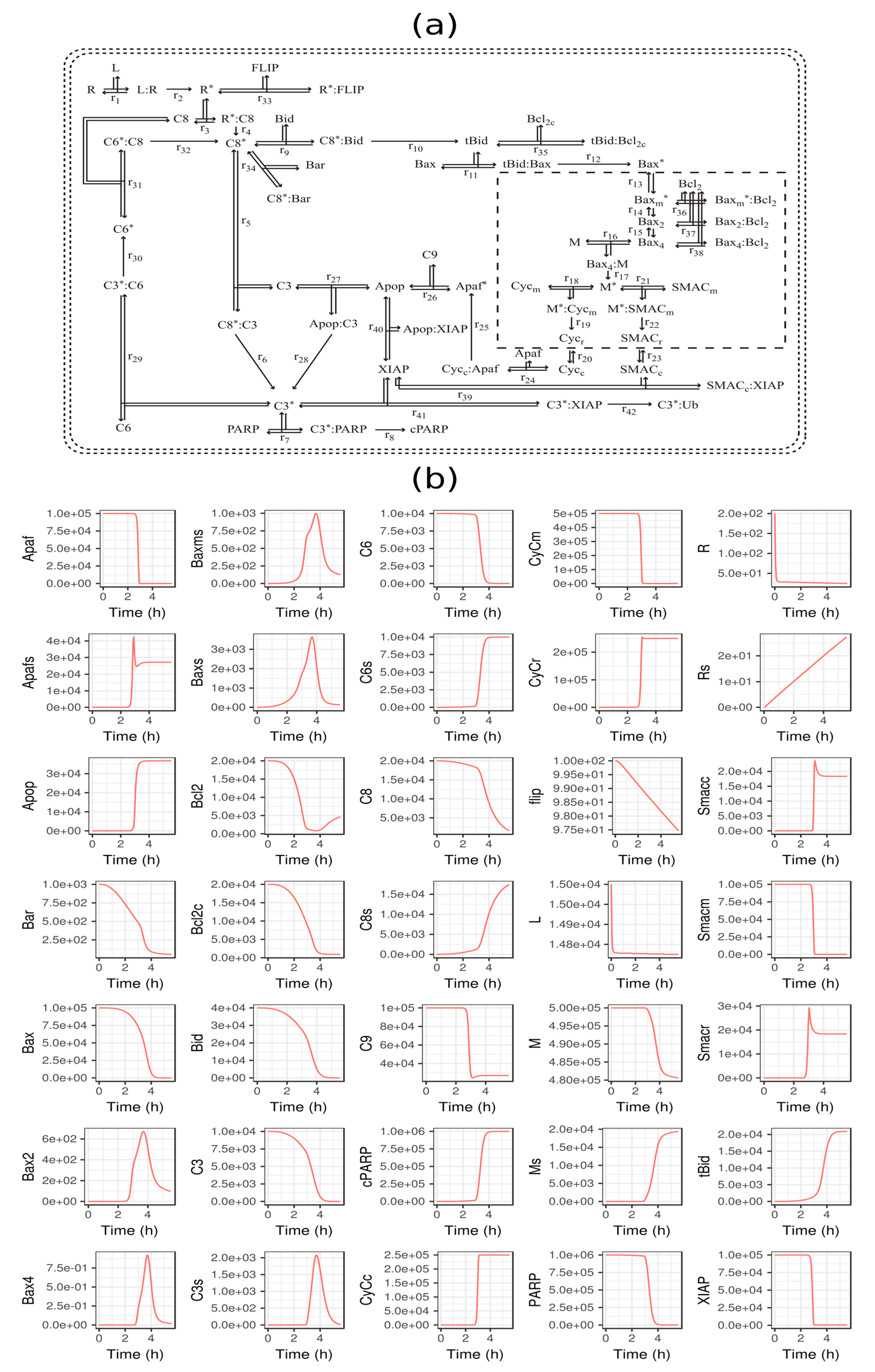
Figure 2 depicts the signaling network associated with extrinsically-induced apoptosis by the tumor necrosis factor-related apoptosis-inducing ligand (TRAIL). The ODE model comprises 58 species, 28 reactions, and 70 kinetic parameters [34] (see Supplementary Material S2 for details on the initial conditions, parameter values, and rate equations). The model parameters and initial conditions were previously determined by parameter fitting to single-cell and cell population data from cell imaging, flow cytometry, and immunoblotting experiments [31,35,36]. The model describes the key mechanisms for the activation of endogenous executioner caspase-3 (C3*) and the subsequent cleavage of poly(ADP-ribose) polymerase (PARP) [35]. Specifically, the model describes four major pathways: (i) the upstream pathway, describing TRAIL-induced cleavage of pro-caspase-8 (C8) to caspase-8 (C8*); (ii) the mitochondrial independent type I pathway, describing the cleavage of pro-caspase-3 (C3) to caspase-3 (C3*) by C8* and the inhibition of C3 by X-linked inhibitor of apoptosis (XIAP); (iii) the mitochondrial-dependent type II pathway, describing the formation of mitochondrial pores promoted by C8*, the consequent release of cytochrome c (Cyc) into the cytosol, the formation of apoptosome (Apop) induced by cytosolic Cyc, and the activation of C3 by apoptosome; and (iv) the pro-caspase-6 (C6) positive feedback loop where active C3* could promote the activation of C8. In the following, we applied the GFM and MDFP sensitivity analysis to elucidate the key processes in the cell death decision making. More specifically, we computed the GFM and MDFP sensitivity coefficients of the cleaved PARP (cPARP) concentration, an indicator of apoptosis, with respect to perturbations in the concentration of molecules involved in the regulation of PARP cleavage in the model, excluding the intermediate complexes.
3.2. GFM Analysis of TRAIL-Induced Cell Death
We applied the GFM analysis to the ODE model using the model parameters in the original report and the median initial concentration from a follow-up publication by the same authors [36] (see Supplementary Material S2). The analysis was performed for a constant TRAIL stimulation over a time range of 0 to 5.3 h, in which the concentrations reached steady state (see Figure 2b). Here, the ODE model simulated an apoptotic cell in which the cleavage of PARP in response to TRAIL occurs in a delayed switch-like manner, as shown in Figure 3a. To study the activation dynamics of cPARP in greater detail, the analysis of the GFM sensitivity coefficients was split into two phases: before and after mitochondrial outer membrane permeabilization (pre- and post-MOMP). Following a previous study [31], we defined MOMP to occur when 10% of the total PARP has been cleaved into cPARP, which in this analysis occurred at 2.36 h (see Figure 2b). Figure 3b,c portrays the ten largest GFM sensitivity coefficients of the cPARP concentration in the pre- and post-MOMP phases, respectively (see Supplementary Figures S1 and S2 for the complete GFM sensitivity coefficients). In the pre-MOMP phase, the ten largest GFM sensitivity magnitudes were associated with the upstream and type I pathways, indicating that the early dynamics of cPARP response to the TRAIL stimulus depends on these two pathways. In the post-MOMP phase, the top sensitivity coefficients corresponded to the type II pathway, specifically the regulators of MOMP (i.e., the signaling molecules upstream of M* in the network in Figure 2). Thus, the GFM analysis indicates that the switch-like dynamics in the cPARP concentration relies on the mitochondria-dependent pathway.
3.3. MDFP Analysis of TRAIL-Induced Cell Death
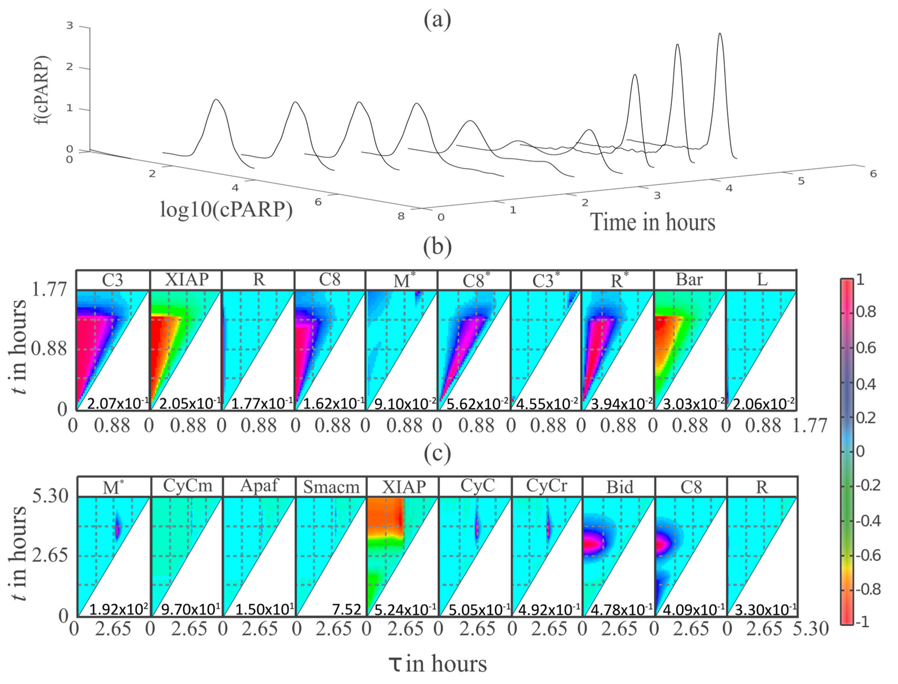
The MDFP analysis was carried out for the same TRAIL stimulation as the GFM. For the calculation of the cell distribution, we generated five ensembles of 1000 initial concentrations from a log-normal distribution using the Latin hypercube sampling (LHS) algorithm based on the reported mean values and coefficient of variations reported previously [36] (see Supplementary Material S2). Figure 4a gives the time evolution of the distribution of the cPARP concentration based on the simulations of the ODE model using the ensemble of initial concentrations. Following the original study [36], we defined cells to be apoptotic when 50% of the total PARP at the final time exists in its cleaved form. The ensemble model simulations showed that on average ~95% of the cells in the simulated cell population undergo apoptosis, similar to what was reported in the original modeling study [36].
As in the GFM analysis above, we computed the MDFP sensitivities of cPARP with respect to perturbations to the concentrations of other molecules in the network. Following Equation (2), we introduced a mean shift perturbation to the distribution of each state variable at various perturbation times , specifically by adding +10% or −10% of the mean concentration to the state variable (i.e., , where is the mean of the state at time ). Starting from the perturbed concentrations, we simulated the time-evolution of cPARP for time . Based on these simulations, we reconstructed the marginal PDFs and CDFs of the cPARP using the kernel density function approximation, which were then used in the calculation of the sensitivity coefficients as prescribed in Equation (6).
Figure 4b,c shows the heatmaps of the ten largest MDFP sensitivity coefficients (in magnitude) averaged over the five ensembles (see Supplementary Figures S3 and S4 for the complete MDFP sensitivity coefficients). We also split the analysis into two phases: pre- and post-MOMP at 1.76 h, the time when the median of cPARP concentration reached 10% of the median of total PARP concentration. Similar to the GFM analysis, the MDFP analysis showed that the early response of cPARP to TRAIL-induced apoptosis depends on the upstream and type I pathway molecules. Meanwhile, the cleavage of PARP in the post-MOMP phase is sensitive to mitochondria-dependent pathway molecules, again confirming the general finding of the GFM analysis above. However, in contrast to the GFM analysis, the MDFP sensitivity coefficients pointed to events during and after MOMP, such as the release of cytochrome c from mitochondria, the binding of XIAP by Smac, and the formation of the apoptosome, as the key regulators of cPARP concentration.
3.4. MDFP Analysis of Apoptotic and Non-Apoptotic HeLa Cells
We repeated the MDFP analysis focusing on the subpopulations of apoptotic and non-apoptotic cells separately. Here, the final cPARP concentration (at time 5.3 h) was taken to be the indicator of apoptosis, where an apoptotic cell has at least 50% of the total PARP cleaved (see Figure 5a,b) [36]. Since only 5% of the population was non-apoptotic, a resampling of the initial conditions was performed to simulate 10,000 cells, from which a population of 1000 apoptotic and 1000 non-apoptotic cells were chosen for MDFP analysis. We then ranked the molecules according to the infinite norm of the MDFP sensitivity coefficients of the final cPARP level with respect to the respective molecular concentrations (i.e., ). Figure 5c,d shows the ranking of the top ten molecules according to the magnitudes of (see Supplementary Figure S5 for the complete MDFP sensitivity coefficients of non-apoptotic cells). The MDFP ranking of the apoptotic subpopulation was in agreement with the GFM analysis in which the final cPARP level depended on the molecules that regulate MOMP. The similarity between the GFM and MDFP analyses of an apoptotic subpopulation is perhaps not surprising considering that the GFM analysis was applied to the model of a cell undergoing apoptosis. Meanwhile, the analysis of a non-apoptotic subpopulation produced a ranking that resembled the outcome of the MDFP analysis of the cell population above. Comparing the analysis of the apoptotic and non-apoptotic cells showed the importance of MOMP, XIAP and its inhibitor Smac, and Apaf-1 in regulating the final cPARP in non-apoptotic cells. Interestingly, among the apoptotic cells, XIAP was not among the 10 largest sensitivity coefficients.
4. Discussion
Cell-to-cell variability has important functional roles in physiological processes, such as cell decision making in stem cell differentiation and cell death. In this work, we developed a sensitivity analysis method called molecular density function perturbation (MDFP) based on introducing time-varying mean shift perturbations to the distribution of molecular concentrations and quantifying the effects of such perturbations on the distribution of the concentration of molecules of interest. The magnitude of the MDFP sensitivity coefficients indicates how much a perturbation to the concentration PDF of one molecule introduced at a particular time affects the concentration PDF of a molecule of interest at some time . We applied the MDFP analysis to a model of programmed cell death signaling in a population of HeLa cells to elucidate the apoptosis decision making. We used the magnitude of the sensitivity coefficients to rank the importance of each molecule in determining the concentration of cleaved PARP, an indicator of apoptosis.
In the application of the MDFP analysis, we employed the Cramer–von Mises distribution distance in the calculation of the sensitivity coefficients. As mentioned in Section 2.1, several alternative distribution distance metrics exist for defining the MDFP sensitivity coefficients. The rankings of molecules based on the cPARP sensitivity coefficients using different distribution distances were strongly correlated with the Cramer–von Mises and with each other (see Supplementary Figure S6a). Furthermore, the ranking of molecules using different perturbation magnitudes (1%, 10% and 100% of the mean) were in agreement with each other (see Supplementary Figure S6b). Thus, the conclusion of the MDFP analysis did not depend strongly on the choice of distribution distance and perturbation size.
Global sensitivity analysis methods such as SOBOL sensitivity [16], DGSM [17], and glocal analysis [18] can be applied to analyze mathematical models of cell populations. As mentioned earlier and explained in [29], the dynamical aspects of cellular regulation may not be immediately apparent from the application of these analyses. Briefly, the reason stems from the fact that the perturbations in these methods are introduced to model parameters in a time-invariant (static) manner. Consequently, the effects of the perturbations on the system behavior are integrated over time [29]. While existing global sensitivity analyses are able to indicate which parametric perturbations cause a significant change in the overall system behavior (output), the sensitivity coefficients do not directly point to when these perturbations matter.
At the cost of requiring more complicated calculations than the existing global sensitivity analysis methods, the MDFP analysis provides dynamic information on the bottlenecking process by revealing the molecular concentrations to which perturbations introduced at time would elicit a large change in a particular state variable of interest at . For example, referring to Figure 4c, the heatmap of the MDFP sensitivity coefficient of cPARP with respect to pro-caspase-8 (C8) indicates that perturbing the distribution of pro-caspase-8 at the beginning of the experiment (h) would cause a much higher impact on cPARP compared to a perturbation delivered after ~2 h. Figure 6 shows the effects of a positive mean shift perturbation to C8 () at two different perturbation times, either h or h, on the mean, median, and standard deviation of cPARP distribution, confirming the MDFP sensitivity analysis.
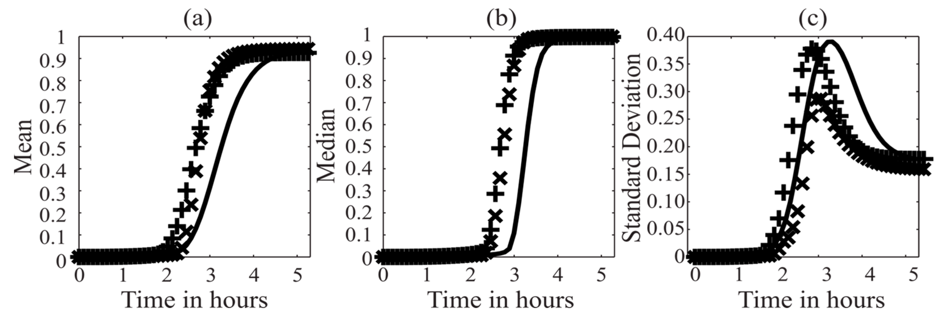
The MDFP analysis of the cell distribution and the GFM analysis of the ODE model provided somewhat different conclusions with respect to the regulation of PARP cleavage. According to the GFM analysis, the switching dynamics of cPARP depends on the molecules upstream of MOMP, particularly the initial level of pro-caspase-8 (C8). On the other hand, the MDFP analysis suggests that PARP cleavage is strongly sensitive to MOMP and the subsequent release of cytochrome c into the cytosolic compartment. As done in Figure 6, we compared perturbing the mean initial concentration of pro-caspase 8 (C8) at the initial time with perturbing the mean number of mitochondrial open pores (M*) at time h, when M* level had reached steady state for more than 99% of the cells. Both perturbations were implemented using 100% positive mean shifts. Figure 7 shows the effects of the above perturbations on the mean, median, and standard deviation of cPARP concentration. As illustrated in Figure 7, both perturbations led to similar shifts in the mean and median of cPARP, where the switch-like dynamic of PARP cleavage occurred earlier and more swiftly. Meanwhile, the perturbation to M* caused a larger drop in the standard deviation of cPARP than the perturbation to C8 (i.e., cells became more alike when we increased the number of mitochondrial open pores). While the positive mean shift perturbation to pro-caspase-8 led to a faster cleavage of PARP, this perturbation did not affect the fraction of apoptotic versus non-apoptotic cells. However, when we increased the number of mitochondrial open pores, the fraction of non-apoptotic cells dropped from 5.6% to 3.2%.
Both the GFM and MDFP analyses of the cell death signaling network implicate the mitochondria-dependent type II pathway to be the responsible mechanism in the switch-like activation of PARP in HeLa cells, placing caspase-8 activation (cleavage) as the most important step in the apoptosis decision making during pre-MOMP. This finding agrees with a previous experimental study on fractional killing by TRAIL [31,37], reporting that the activation of C8 controls the switching time of cPARP. In post-MOMP, the GFM analysis indicates that perturbations to the regulators of MOMP (upstream of M* in Figure 2) would strongly affect the PARP cleavage dynamics. On the other hand, the MDFP analysis points to MOMP and events post-MOMP (downstream of M* in Figure 2), including cytochrome c and Smac release from mitochondria, XIAP binding by Smac, and apoptosome formation, to be the key determinants of the cell-to-cell variability in cPARP level. The finding from the MDFP analysis is in agreement with a previous study that found XIAP to be the determining factor for the rate and extent of type II cell death [38]. Furthermore, the results of the MDFP analysis of apoptotic and non-apoptotic subpopulations showed that perturbations to molecules executing the cell death signal after MOMP (i.e., Smac, cytochrome C, Apaf-1) had a stronger effect on the cPARP activation in the non-apoptotic cells than in the apoptotic cells. Consistent with such an insight, the depletion of Apaf-1 or Apaf-1/Smac together by siRNA has been shown to significantly reduce the activation of PARP in HeLa cells (see Supplementary Figure S7 in [36]).
As the functional significance of cell-to-cell variability is increasingly being recognized and the mathematical models that are able to describe cell distribution become more and more common, the MDFP analysis proposed here will provide an analytical tool to use such models for elucidating the key molecules and processes that govern the dynamics of cellular heterogeneity.
Supplementary Materials
The following are available online at www.mdpi.com/2227-9717/6/2/9/s1, Material S1: Probability distance metrics, Material S2: TRAIL induced programmed cell death model of Hela cells, Figure S1: GFM analysis of TRAIL induced apoptosis model during pre-MOMP (before 2.36 h), Figure S2: GFM analysis of TRAIL-induced apoptosis model during post-MOMP (after 2.36 h), Figure S3: MDFP analysis of TRAIL-induced apoptosis model during pre-MOMP (before 1.76 h), Figure S4: MDFP analysis of TRAIL-induced apoptosis model during post-MOMP (after 1.76 h), Figure S5: MDFP analysis of non-apoptotic Hela subpopulation, Figure S6: Spearman correlations of MDFP sensitivity coefficients using different distribution distances and perturbation sizes.
Acknowledgments
TMP was supported by the Singapore Millennium Foundation scholarship. The authors would like to acknowledge funding from ETH Zurich, as well as support from Sage Bionetworks.
Author Contributions
T.M.P. and R.G. conceived and designed the study; T.M.P. performed the computational work; T.M.P. and R.G. analyzed the data; T.M.P. and R.G. wrote the paper.
Conflicts of Interest
The authors declare no conflict of interest. The founding sponsors had no role in the design of the study; in the collection, analyses, or interpretation of data; in the writing of the manuscript, or in the decision to publish the results.
References
- Cahan, P.; Daley, G.Q. Origins and implications of pluripotent stem cell variability and heterogeneity. Nat. Rev. Mol. Cell Biol. 2013, 14, 357–368. [Google Scholar] [CrossRef] [PubMed]
- Flusberg, D.A.; Sorger, P.K. Surviving apoptosis: Life-death signaling in single cells. Trends Cell Biol. 2015, 25, 446–458. [Google Scholar] [CrossRef] [PubMed]
- Xia, X.; Owen, M.S.; Lee, R.E.C.; Gaudet, S. Cell-to-cell variability in cell death: Can systems biology help us make sense of it all? Cell Death Dis. 2014, 5, e1261. [Google Scholar] [CrossRef] [PubMed] [Green Version]
- Golding, I.; Paulsson, J.; Zawilski, S.M.; Cox, E.C. Real-time kinetics of gene activity in individual bacteria. Cell 2005, 123, 1025–1036. [Google Scholar] [CrossRef] [PubMed]
- Raj, A.; Peskin, C.S.; Tranchina, D.; Vargas, D.Y.; Tyagi, S. Stochastic mRNA synthesis in mammalian cells. PLoS Biol. 2006, 4, e309. [Google Scholar] [CrossRef] [PubMed]
- Raj, A.; van Oudenaarden, A. Nature, nurture, or chance: Stochastic gene expression and its consequences. Cell 2008, 135, 216–226. [Google Scholar] [CrossRef] [PubMed]
- Jia, G.; Stephanopoulos, G.; Gunawan, R. Ensemble kinetic modeling of kinetic metabolic networks from dynamics metabolic profiles. Metabolites 2012, 2, 891–912. [Google Scholar] [CrossRef] [PubMed]
- Stamakis, M. Cell population balance and hybrid modeling of population dynamics for a single gene with feedback. Comput. Chem. Eng. 2013, 53, 25–34. [Google Scholar] [CrossRef]
- Hasenauer, J.; Hasenauer, C.; Hucho, T.; Theis, F.J. ODE constrained mixture modelling: A method for unraveling subpopulation structures and dynamics. PLoS Comput. Biol. 2014, 10, e1003686. [Google Scholar] [CrossRef] [PubMed]
- Henson, M.A. Dynamic modeling of microbial cell populations. Curr. Opin. Biotechnol. 2003, 14, 460–467. [Google Scholar] [CrossRef]
- Hasty, J.; Pradines, J.; Dolnik, M.; Collins, J.J. Noise-based switches and amplifiers for gene expression. Proc. Natl. Acad. Sci. USA 2000, 97, 2075–2080. [Google Scholar] [CrossRef] [PubMed]
- Manninen, T.; Linne, M.L.; Ruohonen, K. Developing Ito stochastic differential equation models for neuronal signal transduction pathways. Comput. Biol. Chem. 2006, 30, 280–291. [Google Scholar]
- Samoilov, M.S.; Arkin, A.P. Deviant effects in molecular reaction pathways. Nat. Biotechnol. 2006, 24, 1235–1240. [Google Scholar] [CrossRef] [PubMed]
- Shahrezaei, V.; Swain, P.S. Analytical distributions for stochastic gene expression. Proc. Natl. Acad. Sci. USA 2008, 105, 17256–17261. [Google Scholar] [CrossRef] [PubMed]
- Poovathingal, S.K.; Gruber, J.; Halliwell, B.; Gunawan, R. Stochastic drift in mitochondrial DNA point mutations: A novel perspective ex silico. PLoS Comput. Biol. 2009, 5, e1000572. [Google Scholar] [CrossRef] [PubMed] [Green Version]
- Saltelli, A.; Ratto, M.; Andres, T.; Campolongo, F.; Cariboni, J.; Gatelli, D.; Saisana, M.; Tarantola, S. Global Sensitivity Analysis. The Primer; John Wiley & Sons: Hoboken, NJ, USA, 2008. [Google Scholar]
- Kucherenko, S.; Rodriguez-Fernandez, M.; Pantelides, C.; Shah, N. Monte Carlo evaluation of derivative-based global sensitivity measures. Reliab. Eng. Syst. Saf. 2009, 94, 1135–1148. [Google Scholar] [CrossRef]
- Hafner, M.; Koeppl, H.; Hasler, M.; Wagner, A. “Glocal” Robustness Analysis and Model Discrimination for Circadian Oscillators. PLoS Comput. Biol. 2009, 5, e1000534. [Google Scholar] [CrossRef] [PubMed] [Green Version]
- Marino, S.; Hogue, I.B.; Ray, C.J.; Kirschner, D.E. A methodology for performing global uncertainty and sensitivity analysis in systems biology. J. Theor. Biol. 2008, 254, 178–196. [Google Scholar] [CrossRef] [PubMed]
- Gunawan, R.; Cao, Y.; Petzold, L.; Doyle, F.J., III. Sensitivity analysis of discrete stochastic systems. Biophys. J. 2005, 88, 2530–2540. [Google Scholar] [CrossRef] [PubMed]
- Komorowski, M.; Costa, M.J.; Rand, D.A.; Stumpf, M.P.H. Sensitivity, robustness, and identifiability in stochastic chemical kinetics models. Proc. Natl. Acad. Sci. USA 2011, 108, 8645–8650. [Google Scholar] [CrossRef] [PubMed]
- Plyasunov, S.; Arkin, A.P. Efficient stochastic sensitivity analysis of discrete event systems. J. Comput. Phys. 2007, 221, 724–738. [Google Scholar] [CrossRef]
- Rathinam, M.; Sheppard, P.W.; Khammash, M. Efficient computation of parameter sensitivities of discrete stochastic chemical reaction networks. J. Chem. Phys. 2010, 132, 034103. [Google Scholar] [CrossRef] [PubMed]
- Gunawan, R.; Jung, M.Y.L.; Braatz, R.D.; Seebauer, E.G. Parameter sensitivity analysis applied to modeling of transient enhanced diffusion and activation of Boron in Silicon. J. Electrochem. Soc. 2003, 150, G758–G765. [Google Scholar] [CrossRef]
- Gunawan, R.; Doyle, F.J., III. Phase sensitivity analysis of circadian rhythm entrainment. J. Biol. Rhythms 2007, 22, 180–194. [Google Scholar] [CrossRef] [PubMed]
- Ingalls, B. Sensitivity analysis: From model parameters to system behaviour. Essays Biochem. 2008, 45, 177–193. [Google Scholar] [CrossRef] [PubMed]
- Zi, Z. Sensitivity analysis approaches applied to systems biology models. IET Syst. Biol. 2011, 5, 336–346. [Google Scholar] [CrossRef] [PubMed]
- Perumal, T.M.; Wu, Y.; Gunawan, R. Dynamical analysis of cellular networks based on the Green’s function matrix. J. Theor. Biol. 2009, 261, 248–259. [Google Scholar] [CrossRef] [PubMed]
- Perumal, T.M.; Gunawan, R. Understanding dynamics using sensitivity analysis: Caveat and solution. BMC Syst. Biol. 2011, 5, 41. [Google Scholar] [CrossRef] [PubMed]
- Perumal, T.M.; Krishna, S.M.; Tallam, S.S.; Gunawan, R. Reduction of kinetic models using dynamic sensitivities. Comput. Chem. Eng. 2013, 56, 37–45. [Google Scholar] [CrossRef]
- Spencer, S.L.; Gaudet, S.; Albeck, J.G.; Burke, J.M.; Sorger, P.K. Non-genetic origins of cell-to-cell variability in TRAIL-induced apoptosis. Nature 2009, 459, 428–432. [Google Scholar] [CrossRef] [PubMed]
- Varma, A.; Morbidelli, M.; Wu, H. Parametric Sensitivity in Chemical Systems; Cambridge University Press: Cambridge, UK, 1999. [Google Scholar]
- Peter, D.H. Kernel estimation of a distribution function. Commun. Stat. Theory Methods 1985, 14, 605–620. [Google Scholar] [CrossRef]
- Niepel, M.; Spencer, S.L.; Sorger, P.K. Non-genetic cell-to-cell variability and the consequences for pharmacology. Curr. Opin. Chem. Biol. 2009, 13, 556–561. [Google Scholar] [CrossRef] [PubMed]
- Albeck, J.G.; Burke, J.M.; Aldridge, B.B.; Zhang, M.; Lauffenburger, D.A.; Sorger, P.K. Quantitative analysis of pathways controlling extrinsic apoptosis in single cells. Mol. Cell 2008, 30, 11–25. [Google Scholar] [CrossRef] [PubMed]
- Albeck, J.G.; Burke, J.M.; Spencer, S.L.; Lauffenburger, D.A.; Sorger, P.K. Modeling a snap-action, variable-delay switch controlling extrinsic cell death. PLoS Biol. 2008, 6, 2831–2852. [Google Scholar] [CrossRef] [PubMed] [Green Version]
- Roux, J.; Hafner, M.; Bandara, S.; Sims, J.J.; Hudson, H.; Chai, D.; Sorger, P.K. Fractional killing arises from cell-to-cell variability in overcoming a caspase activity threshold. Mol. Syst. Biol. 2015, 11, 803. [Google Scholar] [CrossRef] [PubMed]
- Gaudet, S.; Spencer, S.L.; Chen, W.W.; Sorger, P.K. Exploring the contextual sensitivity of factors that determine cell-to-cell variability in receptor-mediated apoptosis. PLoS Comput. Biol. 2012, 8, e1002482. [Google Scholar] [CrossRef] [PubMed] [Green Version]
Figure 1.
A heatmap of the molecular density function perturbation (MDFP) sensitivity coefficient. The x-axis represents the time at which the perturbation is introduced while the y-axis represents the observation time t. The MDFP coefficient in the heatmap is scaled such that the magnitude falls within ±1, and the scaling factor is reported in the lower right corner of the plot. The sensitivity values for are set to zero for causal systems.
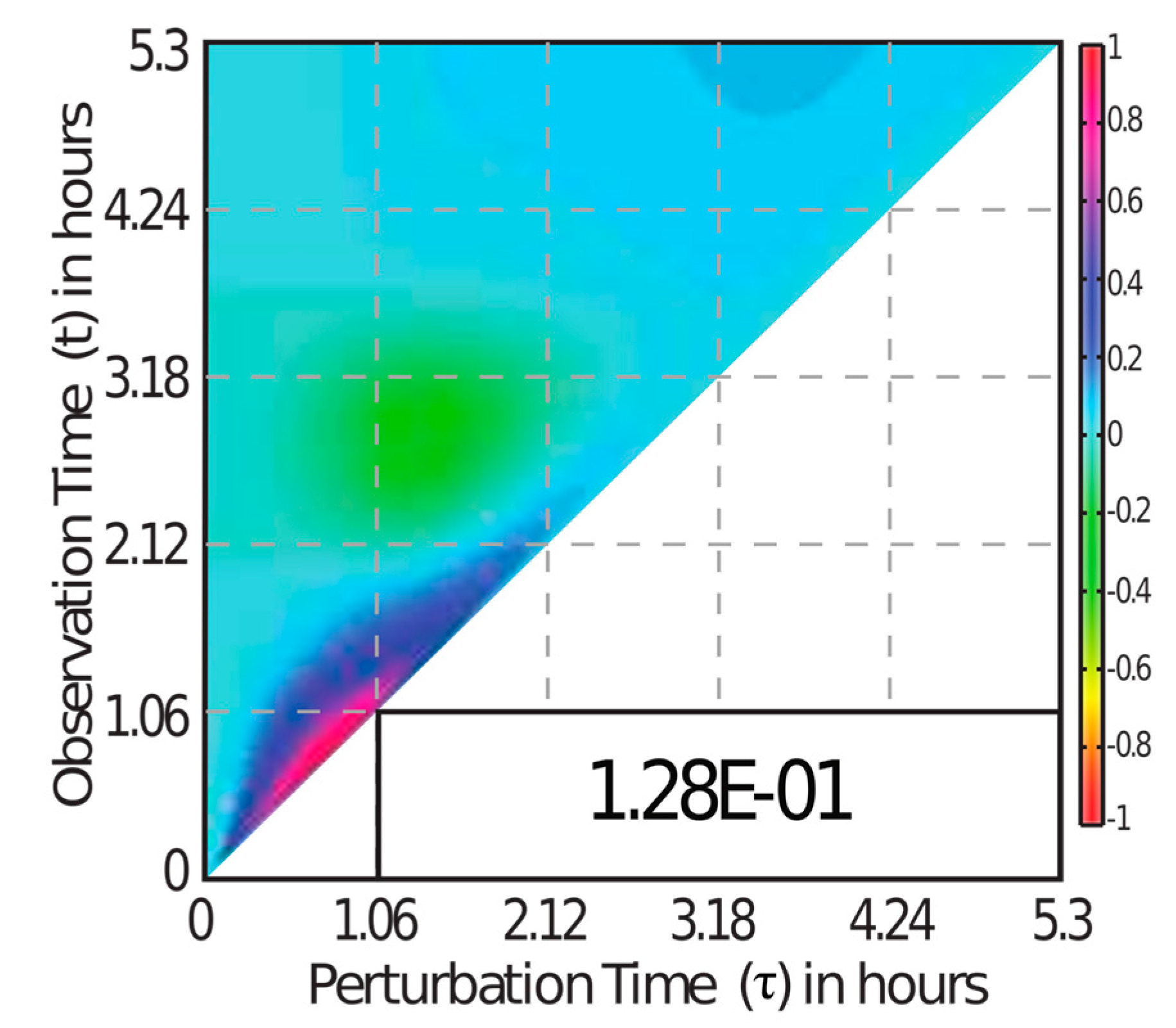
Figure 2.
Signal transduction pathway and model simulation of TRAIL (tumor necrosis factor-related apoptosis-inducing ligand)-induced apoptosis in HeLa cells. (a) Signal transduction pathway of apoptosis. Type I pathway describes the activation of caspase-3 by caspase-8 while type II pathway describes a mitochondria-dependent activation of caspase-3. Active caspase-3 subsequently cleaves the substrate poly(ADP-ribose) polymerase (PARP) to produce cleaved poly(ADP-ribose) polymerase (cPARP). (b) Model simulation of signal transduction pathway in response to TRAIL.

Figure 3.
Green’s function matrix (GFM) analysis of cPARP activation by a constant TRAIL stimulus. (a) cPARP activation follows a delayed switch-like trajectory in response to a constant TRAIL stimulus. (b,c) Ten largest GFM sensitivity coefficients of cPARP concentration (in magnitude) with respect to perturbations to the state variables in the network, as shown on the label of each subfigure. The x-axis gives the time of perturbation while the y-axis represents the time of observation . Each heatmap is scaled to have values within ±1, using the scaling factor reported in the lower right corner of the plot. Panel (b) shows the GFM sensitivity coefficients in the pre-MOMP phase (before 2.36 h). Panel (c) shows the GFM sensitivity coefficients in the post-MOMP phase (after 2.36 h).
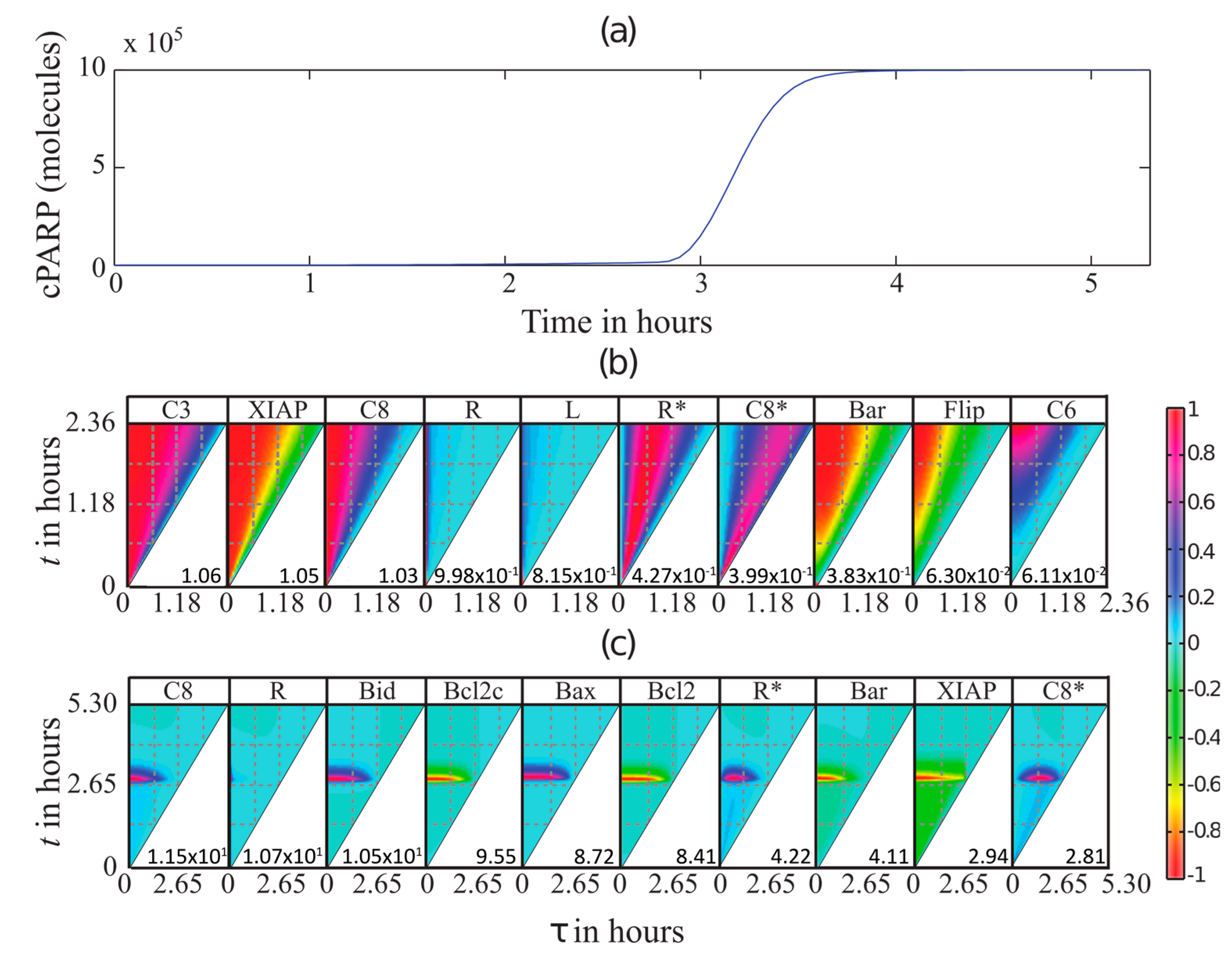
Figure 4.
MDFP analysis of cPARP activation by a constant TRAIL stimulus. (a) Time evolution of the distribution of cPARP concentration shows a switch-like behavior. (b,c) Ten largest MDFP coefficients of cPARP concentration (in magnitude) with respect to the perturbations to different state variables in the network. The x-axis gives the time of perturbation while the y-axis gives the time of observation . Each heatmap is scaled to have values within ±1, using the scaling factor reported in the lower right corner of the plot. Panel (b) shows the MDFP sensitivity coefficients pre-MOMP (until 1.76 h). Panel (c) shows the MDFP sensitivity coefficients post-MOMP.

Figure 5.
MDFP analysis of the final cleaved PARP levels in (a,c) apoptotic and (b,d) non-apoptotic cell subpopulations. (a,b) The level of cPARP normalized with respect to the total PARP level. The dashed lines (--) indicate the 1 and 99 percentiles of the cPARP levels, while the solid line (-) represents the median level. (c,d) Ten largest sensitivity coefficients in magnitude in apoptotic and non-apoptotic cells, respectively.
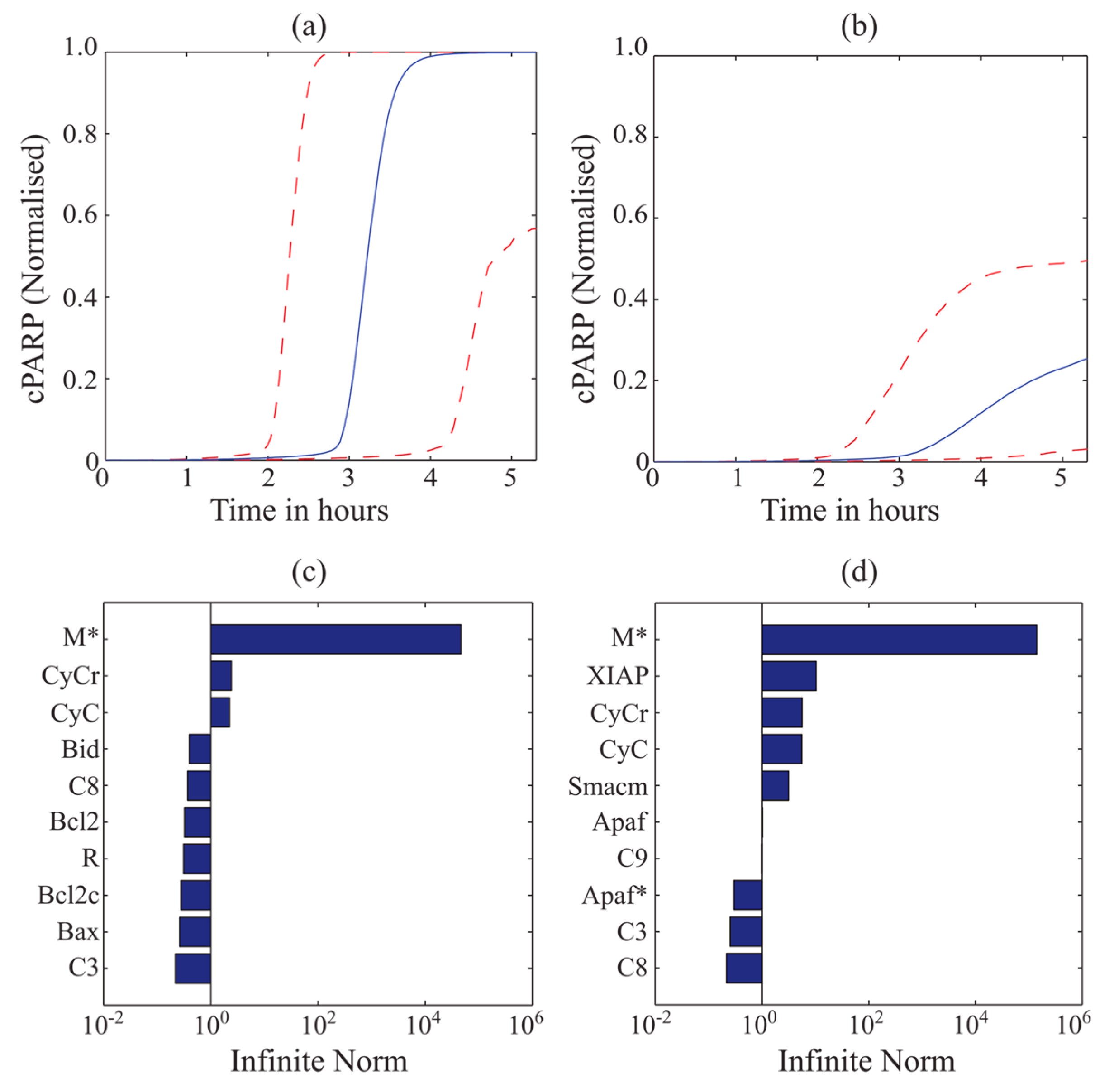
Figure 6.
Validation of the MDFP sensitivity analysis of cPARP. A positive mean shift perturbation to pro-caspase-8 was given either at h (+) or at h (). Panel (a) shows the mean; panel (b) gives the median; and panel (c) gives the standard deviation of the cPARP concentration. The unperturbed simulation is shown as solid lines ().
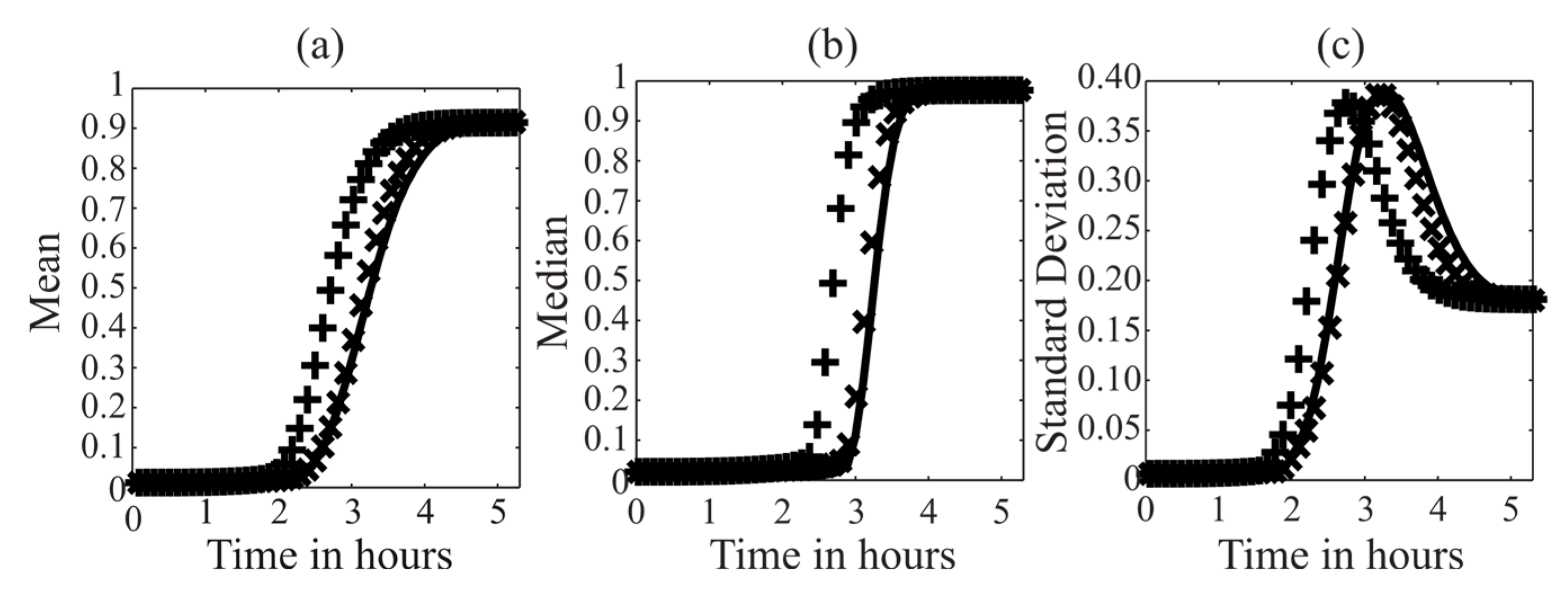
Figure 7.
Comparison of GFM and MDFP analyses. A positive mean shift perturbation was given either to pro-caspase-8 a h (+) or to mitochondrial open pores M* at h (). Panel (a) shows the mean of the cPARP concentration distribution, panel (b) gives the median, and panel (c) gives the standard deviation. The unperturbed simulation is shown as solid lines ().
© 2018 by the authors. Licensee MDPI, Basel, Switzerland. This article is an open access article distributed under the terms and conditions of the Creative Commons Attribution (CC BY) license (http://creativecommons.org/licenses/by/4.0/).
Share and Cite
MDPI and ACS Style
Perumal, T.M.; Gunawan, R. Elucidating Cellular Population Dynamics by Molecular Density Function Perturbations. Processes 2018, 6, 9. https://doi.org/10.3390/pr6020009
AMA Style
Perumal TM, Gunawan R. Elucidating Cellular Population Dynamics by Molecular Density Function Perturbations. Processes. 2018; 6(2):9. https://doi.org/10.3390/pr6020009
Chicago/Turabian StylePerumal, Thanneer Malai, and Rudiyanto Gunawan. 2018. "Elucidating Cellular Population Dynamics by Molecular Density Function Perturbations" Processes 6, no. 2: 9. https://doi.org/10.3390/pr6020009
Note that from the first issue of 2016, this journal uses article numbers instead of page numbers. See further details here.