Solving Materials’ Small Data Problem with Dynamic Experimental Databases


School of Chemical and Biomolecular Engineering, Georgia Institute of Technology, Atlanta, GA 30332, USA
*
Author to whom correspondence should be addressed.
Processes 2018, 6(7), 79; https://doi.org/10.3390/pr6070079
Submission received: 7 June 2018
/
Revised: 24 June 2018
/
Accepted: 25 June 2018
/
Published: 27 June 2018
(This article belongs to the Special Issue Feature Papers for the Fifth Year Anniversary of the Founding of Processes)
Abstract
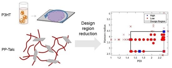
:Materials processing is challenging because the final structure and properties often depend on the process conditions as well as the composition. Past research reported in the archival literature provides a valuable source of information for designing a process to optimize material properties. Typically, the issue is not having too much data (i.e., big data), but rather having a limited amount of data that is sparse, relative to a large number of design variables. The full utilization of this information via a structured database can be challenging, because of inconsistent and incorrect reporting of information. Here, we present a classification approach specifically tailored to the task of identifying a promising design region from a literature database. This design region includes all high performing points, as well as some points having poor performance, for the purpose of focusing future experiments. The classification method is demonstrated on two case studies in polymeric materials, namely: poly(3-hexylthiophene) for flexible electronic devices and polypropylene–talc composite materials for structural applications.
1. Introduction
Research institutions and their funding sources have made a strong push in recent years to leverage the tools of modern data analytics for scientific research. This effort has fostered the creation of large centralized data repositories, the proliferation of more open-source software and code libraries, and a general move toward ‘open science’ [1]. The tools of data analytics and informatics were developed to analyze truly massive databases containing millions to billions of entries, such as the collective Google search history of a country’s population, or the Amazon shopping history of the same. As such, early efforts in the sciences have focused on the assembly of the largest possible collections of data, namely: thermodynamic constants for every known chemical compound, density functional theory (DFT) simulations of every known crystalline material, or characterization data from every known biological protein [2,3,4,5,6].
While the scope of these centralized databases is vast, they still do not capture the full extent of the scientific data collected and published on a daily basis. Day-to-day research is not driven by a desire to fill in the billionth row of a central repository, but rather to solve problems and produce knowledge in specialized fields with moderately-sized communities and dynamic trends. The design of a new research study is most often based upon the results of a few dozen previous studies at most. This would not be considered ‘big data’ by any measure, yet these small sets of experimental results play a crucial role in daily decision-making. In order to use data analytics to guide this decision-making process, it would be beneficial if the datasets from related publications were assembled into interim databases with a common schema. It is likely that many researchers already aggregate data in this way, especially for a formal literature review. This is all the more reason to develop tools and strategies to work quantitatively with these small, sometimes sparse datasets.
Experimental research in materials processing depends crucially on the selection of a promising initial design region within the available process parameters. When processing a material, there are many potential design variables by which to optimize its properties and performance, including formulation, equipment selection, and settings. The challenge of process design for materials differs from chemical production, because the process influences the material’s structure, which further influences its properties. Some crystalline solids and disordered liquids are processed to reach an equilibrium structure, but many materials, such as the soft materials presented here, are guided to process-dependent non-equilibrium states, sometimes with multiple phases. Furthermore, interfacial structures can often influence or even dictate the final performance beyond the bulk material properties. Selecting a process variable design space for a new experiment should thus be approached using as much quantitative knowledge as possible [7].
Data mining approaches to experimental design have experienced a recent uptick in interest. For example, Kim et al. performed an automated review of the synthesis conditions of metal oxides across over 12,000 manuscripts. Their data extraction pipeline consisted of a combination of trained machine learning models and software such as ChemDataExtractor. A decision tree classifier considering 27 synthesis variables was trained to predict whether or not a titania synthesis route would produce nanotubes, achieving 82% accuracy [8]. Agrawal et al. compared a range of machine learning approaches, including multivariate polynomial regression (R2 = 0.9801), support vector machines (R2 = 0.9594), and artificial neural networks (R2 = 0.9724), to predict the fatigue strength of steels [9]. Input variables describing chemical composition, processing temperatures and times, and upstream processing details were taken from the National Institute of Materials Science (NIMS) MatNavi [10]. Ren et al. combined literature data and high-throughput experiments to predict the likelihood of finding metallic glasses in the Co–V–Zr ternary [11].
The use of the design of experiment methodologies to generate ideal process–property databases is another approach to enable subsequent data mining of process–property relationships. This is exemplified by AbuOmar et al. and Zhang et al., where polymer nanocomposite databases were generated via carefully designed experiments [12,13]. The databases generated using uniform design approaches typically only survey low-dimensional design spaces with a priori domain knowledge to appropriately grid experimental values [14]. The common element among these previous studies is the accessibility of fully informed databases with all descriptors fully characterized and reported.
The scientific literature can be conceived as an unstructured materials database, rich with process–property data points. However, the nature of exploratory materials discovery suggests a high-dimensional design space, with individual publications providing a limited number of data points. There are several challenges in constructing and analyzing a literature database, even with manual construction by domain experts, namely: (1) literature reports do not have standardized fields for frequently-reported quantities; (2) authors report non-overlapping sets of information, leading to data sparsity; and (3) reporting of design variables and property measurements suffer from variability due to measurement equipment, inconsistent application of mathematical models, and human error [15]. Persson et al. provides an illustrative example of these challenges by mining the literature on poly(3-hexylthiophene) organic field effect transistors [16]. Over 200 data points from 19 publications describing the role of 28 processing variables were curated to predict charge carrier mobility. Identifying a subset of the five most similar devices reduced the range of charge carrier mobility values from over six orders of magnitude to three. The presence of unreported, missing data limited the applicability of the standard classification and regression materials informatics techniques.
Herein, we demonstrate how the construction of a structured database containing relevant literature results can be used to guide experimental design for materials processing. This tailored approach to classification is proposed to specifically handle datasets with missing data, but is also applicable to fully characterized databases. The set of best performing points indicates a promising design region for future experiments. Two case studies are presented to demonstrate the approach, with each database containing 100–200 data points. The number of data points is largely governed by the available relevant publications. The analysis is primarily intended to guide future experiments into regions likely to have the desired properties. Further local optimization can then be performed using response surface methodology [17,18]. Once the optimal point is identified, then additional design variables could be added to enable further improvement, or previously unexplored regions could be explored.
2. Materials and Methods
2.1. Database Construction
The databases are constructed manually using a Microsoft Excel spreadsheet. The data extracted from relevant publications is found in text, tables, and graphical format. Each row in the spreadsheet corresponds to a particular data point. The columns represent the process design variables, which may be numerical (continuous or integer) or categorical. In some cases, the categorical variables (e.g., solvent type) are augmented with numerical descriptors to quantify their properties (e.g., solvent boiling point). In other cases, the categorical variables are hierarchical (e.g., deposition method: spin-coat) with associated numerical values quantifying that category (e.g., spin rate and spin time). Each property measurement is also associated with a column. Additional columns are included so as to document the source of each datapoint, including its digital object indicator (DOI). Further metrics of the journal impact factor and the number of citations of the paper can also be included, but present additional complications as they change over time.
While this manual, ad hoc approach is not ideal from a scalability standpoint, the cost of automating this step can be prohibitive in terms of time and expertise. Furthermore, the automation of data extraction requires a significant number of labeled training examples, and the construction of the training set frequently accomplishes so much of the labeling that it makes more sense to simply finish the job manually. This trade-off should be evaluated on a case-by-case basis.
2.2. Classification Approach
A common approach to the classification of data is the support vector machine (SVM), which, in its simplest form, constructs a hyperplane to divide two prelabeled classes. This approach is exemplified by Kim et al., who separated metal oxide structures into nanotube-forming and non-nanotube-forming by their processing conditions [8]. SVMs are optimized to maximize the distance between the decision boundary and the nearest point from each class. In other words, SVMs try to minimize the occurrence of misclassification on both sides of the boundary. In exploratory research, however, it is much worse to exclude a potential positive result from consideration than it is to run an experiment that turns out negative. Here, we apply a different approach to classification, in which the objective is to retain all datapoints with good properties in the ‘promising region’.
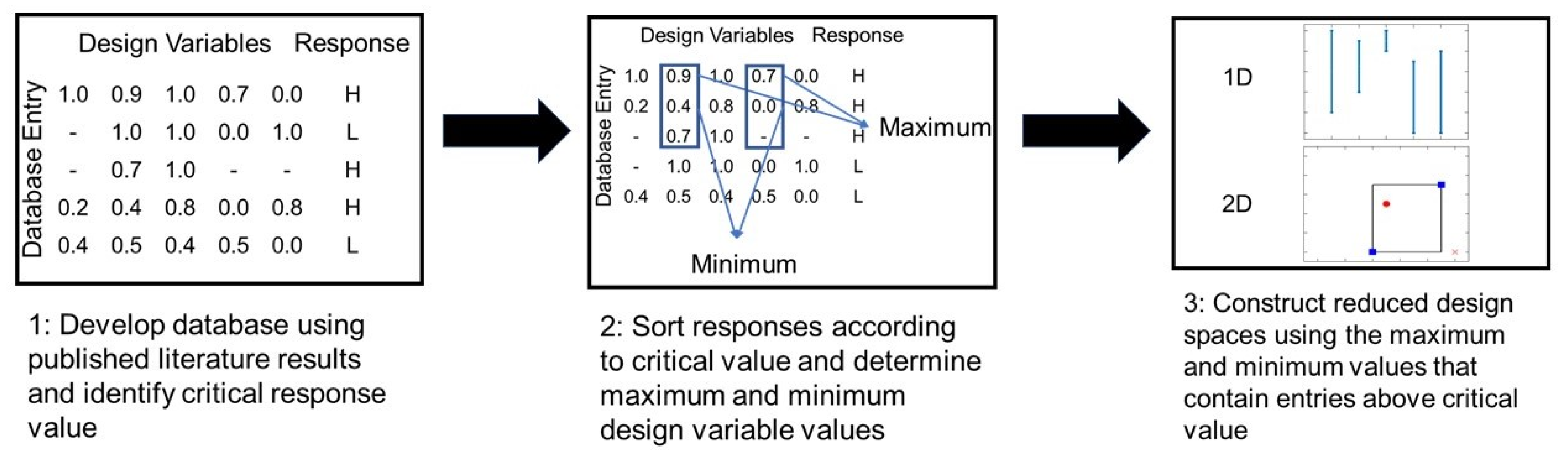
A property of interest is selected, then a critical value of that property is specified by the user. All datapoints in the database are thus labeled as ‘high’ or ‘low’, depending on whether they lie above or below this critical value. The region of the design space that contains all the ‘high’ points is then constructed. Figure 1 illustrates this classification approach. This approach helps to ensure that potential positive results are never excluded from the promising region. It is, however, inherently sensitive to outlier points, in which a ‘high’ property value has been incorrectly reported. These outliers should be uncommon, because such results would most likely have received great interest and scrutiny in the review process. Nonetheless, points with a reported ‘high’ performance should receive further investigation in subsequent experiments, that is, they should be repeated to validate (or invalidate) their good performance.
One possible implementation for quantifying the promising region is to construct a convex hull containing all of the ‘high’ points in the literature database. Here, we take a simpler approach, which is to calculate the upper and lower bounds of each design variable within which all of the ‘high’ points are contained, defining a box. The rationale is to provide better intuition and visualization for the user. For each design variable, one compares the minimum and maximum values for ‘high’ performance to the minimum and maximum values in the entire database, quantifying the percent reduction of the design space, which can be achieved by focusing future experiments on past ‘high’ performing regions. This reduction rs can expressed mathematically, as follows:
where S is the set of indices for a subset of the design variables, ns is the dimensionality of the design space (equivalent to the size of S), li is the span of variable i that contains ‘high’ points, and Li is the span of variable i over all points in the database. In the one-dimensional (1-D) case, rs is the relative length of the line segment that contains the ‘high’ points, while in the two-dimensional (2-D) case, rs is the relative area that contains the ‘high’ points. Each design variable, or combination of design variables, is then represented with a value of rs between 0 and 1, where it is hypothesized that a smaller value signifies that the associated design variable is a better indicator of a ‘high’ performance.
While rs expresses the volumetric reduction of the design space, it is also useful to understand the fraction of the original data contained in the promising region, as data density is likely non-uniform. This is expressed as follows:
where d is the number of points contained within the box and D is the total number of observations in the database. Each observation corresponds to a row in the Excel database spreadsheet.
It is certainly possible that the box excludes potential regions of high performance that were not investigated in previous studies. One could apply a padding parameter to the box bounds to reduce this risk. Alternatively, future experiments can explore additional regions, locally, through response surface methodology, or more globally, with random experimental settings or a particular focus on unexplored regions. Certainly, physical models and domain expertise will also guide future experiments, but the details of the experimental design are beyond the scope of this article [17,18,19].
2.3. Case Studies
2.3.1. Poly(3-Hexylthiophene) (P3HT)
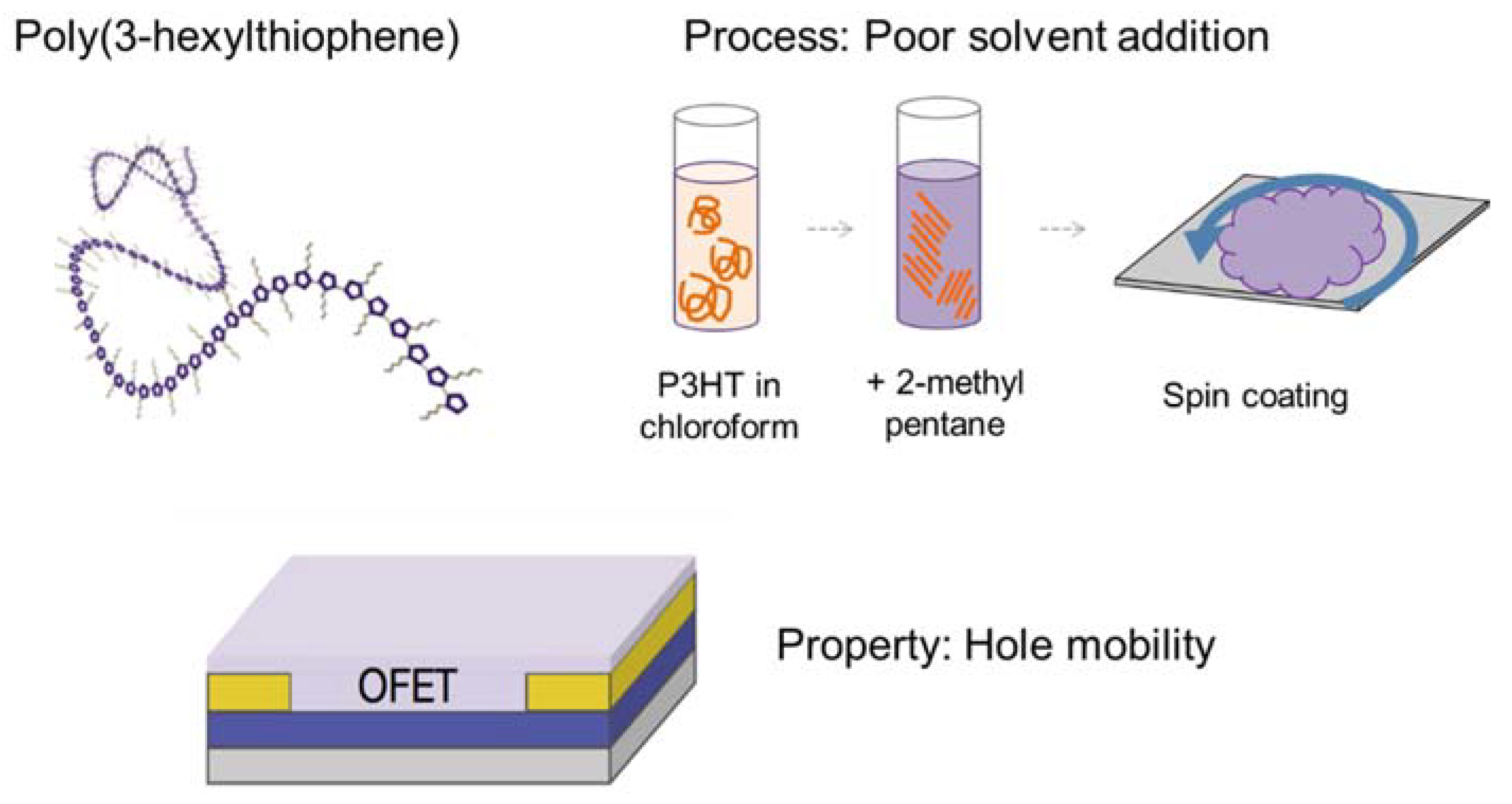
Poly(3-hexylthiophene) is a semiconducting polymer that has been widely studied for application in large-area flexible electronics [20]. Such systems could access new markets beyond silicon transistors if they can be printed economically in a roll-to-roll process. Thin films of P3HT exhibit hole mobilities that vary by orders of magnitude, depending on how they are processed [21]. Distinct fibrillar morphologies are observed in the atomic force microscopy, and the morphology can be influenced by the process, and correlated with the hole mobility [22,23]. Design variables that are reported in the literature include polymer molecular weight and regioregularity, solvent and concentration, deposition method and film thickness, and annealing time [16]. This system is depicted in Figure 2.
The analyzed database, which was presented in a previous publication, is comprised of 218 datapoints from 19 publications. To model process–property relationships to obtain high mobility devices, 29 design variables were identified that are either numerical (20 design variables) or categorical (9 design variables). The design variables were removed from consideration if all relevant entries were identical, exceptionally sparse, or deemed irrelevant according to expert opinion (e.g., dip rate, dip time, process environment, and electrode material). The mobility values in this database range from 1.0 × 10⁻⁶ to 2.8 × 10⁻¹ cm2/V·s.
This database is included in the supplementary information and is also publicly accessible at: http://www.github.com/Imperssonator/OFET-Database.
2.3.2. Polypropylene–Talc Composite
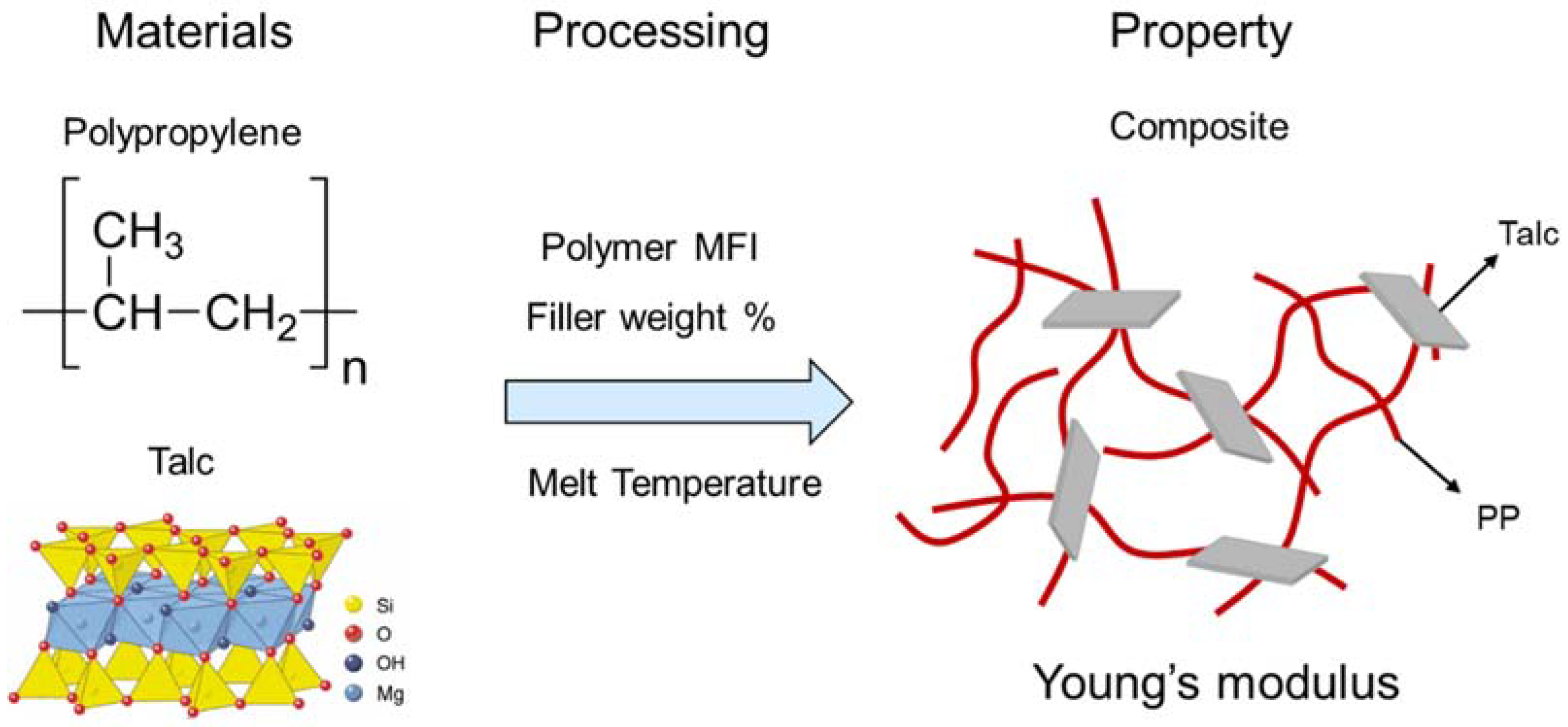
The properties of polymeric materials can be altered and improved by mixing them with fillers to create a composite material [24,25,26]. In addition, the processing method impacts the properties [27]. Polypropylene (PP) has relatively strong mechanical properties for a polymer and it is widely available. If its properties could be further enhanced, polypropylene might be a candidate for replacing metals, for example in the additive manufacturing of automotive parts. Here, we consider talc as our filler. Talc is a clay material composed of magnesium silicate. It is a good filler candidate for our study because it has been reported to enhance polypropylene performance in many literature studies and because it is relatively inexpensive, enhancing commercial viability [28,29]. This system is illustrated in Figure 3.
The polypropylene-talc database is comprised of 140 datapoints from 22 publications with the goal of improving the strength of polypropylene. The Young’s modulus was selected as the relevant mechanical parameter representing the materials’ strength. Fourteen design variables were selected for this analysis, with eleven being numerical and three being categorical. Expert opinion was leveraged to characterize differing melt mixer equipment by recording the highest temperature in a multistate extruder. The Young’s modulus values for this database vary from 0.38 to 6.94 GPa.
This database is included in the supplementary information and is also publicly accessible at: https://github.com/DocMike/TALC-Database.
3. Results
3.1. Case Study 1: Poly-3-Hexylthiophene
The breadth of processing conditions recorded in the P3HT database illustrates the utility of the proposed classification approach. In this database, a mobility cutoff value of 0.1 cm2/V·s was selected to differentiate between ‘high’ and ‘low’ devices. The design variables extracted from the literature can be grouped into five main categories, namely: (1) polymer characteristics, (2) solvent environment, (3) deposition conditions, (4) post-deposition processing, and (5) transistor configuration. All of these variables have been hypothesized to influence the morphology of the final semiconducting film and thus the charge carrier mobility [30,31].
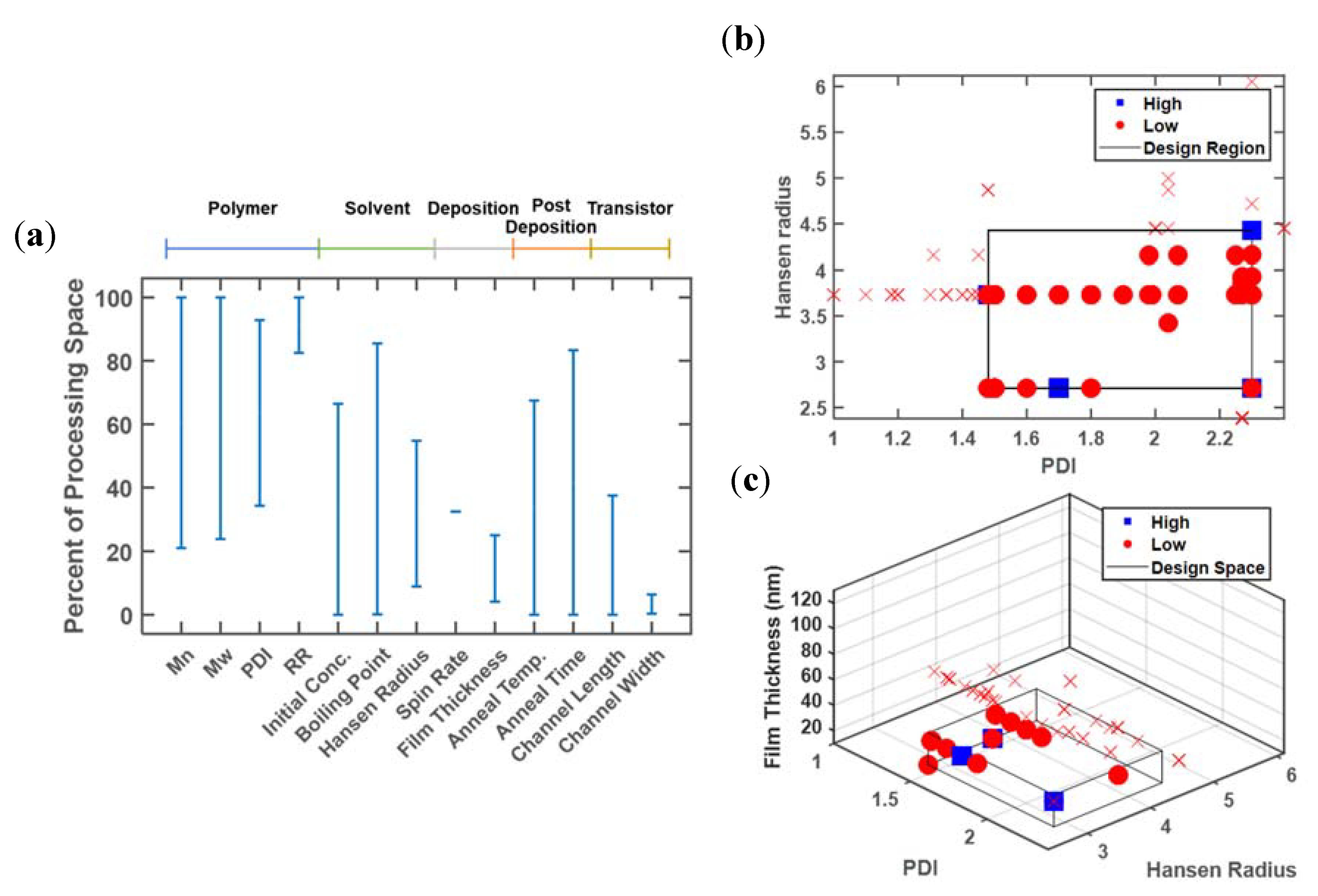
Figure 4 illustrates the classification approach applied to the P3HT database for 13 of the continuous design variables contained in the database, out of a total of 29 design variables of numerical and categorical type. The one-dimensional analysis is shown in Figure 4a for these 13 design variables, with results scaled to the full range of values reported in the database. For each of these design variables, the difference between the maximum and minimum values associated with a ‘high’ performance li, is divided by Li, the difference between the maximum and minimum values associated with all entries in the database, according to Equation (1). In some cases, a ‘high’ performance is observed only for a small fraction of the full reported range, such as for regioregularity, spin rate, and channel width, such that rs < 0.1. In other cases, a ‘high’ performance can be observed at most of the reported values (molecular weight, initial concentration, boiling point, annealing temperature, and time), such that rs > 0.9. In other intermediate cases, a restricted range can be observed, namely: polydispersity, Hansen radius, film thickness, and channel length.
One might first focus on regioregularity, spin rate, and channel width to reduce the design space for future experiments. However, these are not the best candidates. Regioregularity must be high for a ‘high’ performance, which is well known; only a small number of the earlier papers used polymers with lower values of regioregularity [32,33]. Moreover, precision synthesis and characterization of a specific regioregularity is infeasible [34]. Of the 37 ‘high’ devices, only 8 report a spin rate and all 8 arise from the same publication. Thus spin rate is not an ideal candidate. The channel width is also shown to impact the observed mobility, but device physics indicate that it should not influence the transistor performance [35]. The standardization of test conditions is necessary to improve the quantification of results in polymer organic electronics, and future experiments should conform to this common standard [36].
The more revealing design variables are those with a moderate reduction of the design space, namely: polydispersity, Hansen radius, film thickness, and channel length. Like channel width, channel length affects performance through device physics rather than material properties, and can be excluded. This leaves three key design variables, which can be visualized in two or three dimensions, as shown in Figure 4b,c. A high value of polydispersity is required to achieve a good performance, but low values of the Hansen radius and film thickness are also needed.
The two-dimensional plots can be generated for each pairwise combination of design variables, or on the selected promising design variables identified in the one-dimensional analysis. Figure 4b delineates the promising design region using the polymer polydispersity index (PDI) and Hansen radius. The area of the identified design region relative to the full area spanned by the design variables is quantified by rs = 0.27, for S = {3,7}. Thus, future experimental efforts can be focused on only 27% of the original design region. When film thickness is additionally added as a classifier, rs = 0.056, for S = {3,7,9}.
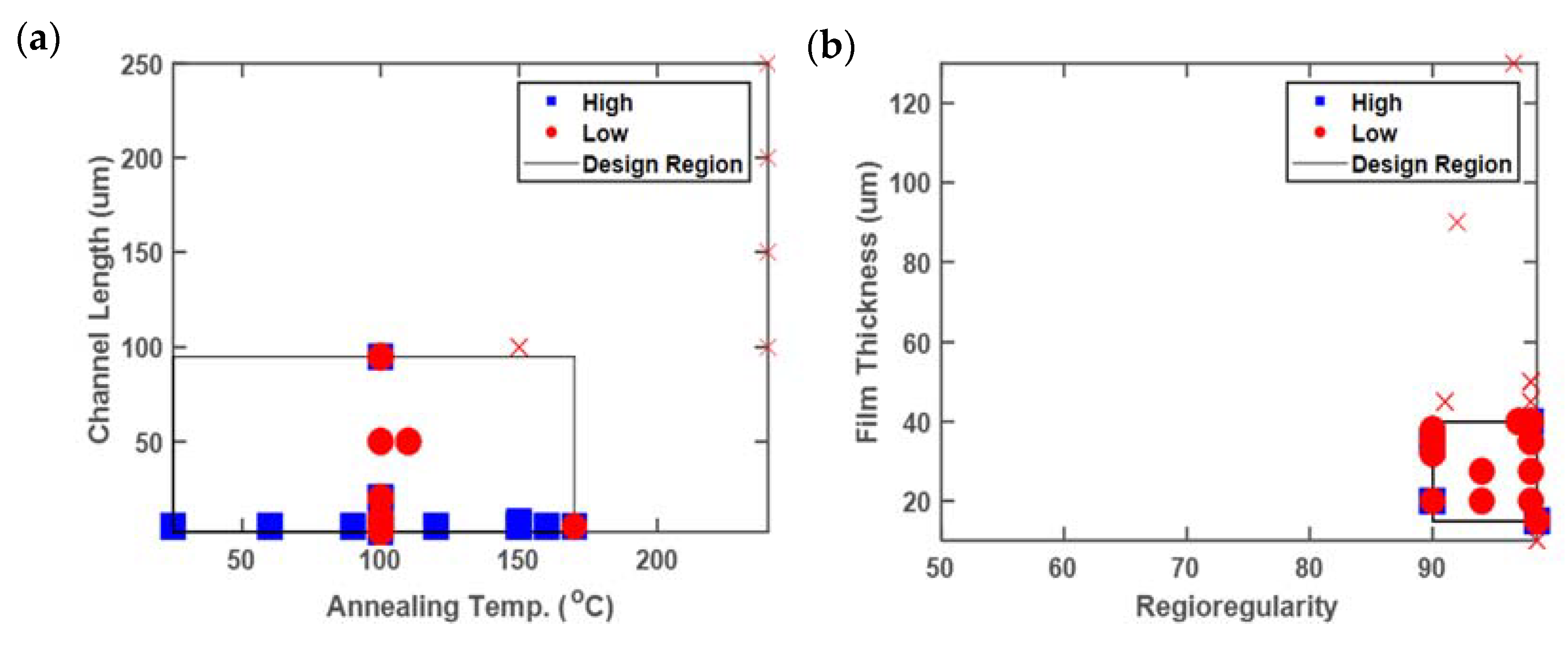
However, quantifying the reduction using rs without visualizing results or utilizing additional metrics can lead to misleading conclusions, depending on the quality of the information in the database. Issues with only characterizing the relative reduction can be grouped into two main categories, as follows: (1) limited coverage of the entire design region (sparsity), and (2) inconsistent reporting and characterization. These cases are illustrated in Figure 5. Note that in Figure 5b, there are no datapoints shown with regioregularity (RR) values below 90%, despite their presence in the database, because film thickness was not reported for any of those datapoints.
The fraction of points contained within the reduced designed region (Fr) serves as a simple indicator for the distribution and sparsity of points throughout the entire design region. Table 1 highlights both the reduced area and the fraction of points contained in this region. In general, rs is smaller than Fr, indicating that the volumetric reduction of the design space is greater than the fraction of database points excluded. This can be rationalized in the context of Schrier’s Dark Reaction Project; negative results are infrequently reported in the literature [37]. It makes sense that data density would be concentrated in the promising region, because other experimentalists intuitively concentrate their effort in a similar region, and because they omit negative results from outside that region. This is a source of significant bias in the training set, but it can also serve as a sanity check on the selection of the promising region. Nonetheless, the importance of reporting negative results cannot be overstated.
This classification approach can theoretically be scaled to any dimension. However, the reliability of the identified target region containing high performing devices decreases as the dimensions increase. This reliability issue is illustrated in Figure 4c with a box denoting the target design region. The data is distributed throughout the x and y plane (PDI and Hansen radius), indicating that these two variables are highly reported. In contrast, no results are presented with a thickness greater than ~40 nm, despite thickness values as high as 130 nm being reported in the database. This problem arises from a lack of standardized reporting. Despite the fact that 146 of the entries report PDI, 190 report Hansen radius values, and 149 report film thickness, only 105 entries have all three of these variables specified. This issue can also impact the relative volume of the target design region. While the two-dimensional analysis (Figure 4b) points to a ‘high’ device with a PDI value of ~2.3 and a Hansen radius of ~4.5, this database entry does not contain a corresponding film thickness and as a result does not appear in Figure 4c. Thus, the analysis of higher-dimensional design spaces to simultaneously optimize numerous processing conditions relies heavily upon consistent and standardized reporting.
In addition to the 13 numerical design variables, three relevant categorical variables were identified. The choice of solvent influences the ability of the polymer chains to self-assemble in the solution and the solvent evaporation rate during the film deposition phase. The analysis performed in this study indicated that the use of chloroform and trichlorobenzene result in ‘high’ performing devices, while toluene, thiophene, benzene, chlorobenzene, and styrene do not. Section 3.1.2 will discuss how solubility parameters (Hansen radius) were used to represent a solvent on a continuous scale. Of the 37 ‘high’ performing devices, 28 films were formed through drop casting, 8 via spin coating, and 1 film using dip casting, spanning all deposition methods in the database. It is likely that the interaction of these deposition methods with other process variables was optimized to produce favorable thin film microstructures. Finally, the treatment of the silicon dioxide capacitance layer to modify the wettability and polymer-substrate interface using hexamethyldisilane (HMDS) or no treatment at all can both result in ‘high’ devices. In contrast, perfluorodecyltrichlorosilane (FDTS) and octadecyltrichlorosilane (OTS) surface treatments produced unfavorable results. Ideally, surface free energy would be reported as a way to quantify the surface treatment, similar to the Hansen radius for the solvent.
Once the target design region has been identified, hypothesis generation and future experiment planning can occur. Here, we briefly discuss the physical intuition that can guide experimental design beyond the selection of the promising design region.
3.1.1. Polydispersity Index
Long polymer chains are required to extend across grain boundaries and thus provide high-mobility pathways through otherwise amorphous regions of the film [33,38,39]. The one-dimensional analysis of polymer characteristics (Figure 4a) suggests that ‘high’ performance devices can be obtained with number average molecular weights ranging from 26 kDa to 117 kDa. The PDI indicates the spread of the molecular weight distribution in a polymer sample, so a sample with a low average molecular weight could still contain many long chains if it has a high PDI. Our analysis indicates that a PDI > 1.5 is required for a high-performance device. However, there is experimental difficulty in synthesizing polymers with tailored PDIs for systematic studies [34]. Instead, techniques to either fractionate the P3HT samples or blend multiple polymers samples to target a specified PDI have been employed [40,41].
3.1.2. Hansen Radius
Thin film formation is a complex and dynamic process in which solvent evaporation governs structural organization mechanisms such as polymer aggregation and phase separation [42]. These processes are captured, albeit incompletely, through the initial polymer concentration, solvent boiling point, and Hansen radius, in addition to the equipment deposition parameters (e.g., spin rate, spin time). According to the one-dimensional analysis, the Hansen radius provides better discrimination between high and low performance devices compared with both the initial polymer concentration and the boiling point. The Hansen radius is a numerical descriptor of solvent–polymer interaction energy and can be used to reduce the number of design variables when solvent mixtures are utilized [11,43,44,45]. As an example, the dissolution of P3HT in a good solvent, followed by the addition of a poor solvent, was utilized as a processing method by 3 of the 19 papers in the database [43,45,46]. To fully characterize this, two categorical variables (good solvent, poor solvent) and one numerical variable (volume fraction of poor solvent) need to be specified. By applying the Hansen solubility model, these three variables can instead be reported as a single numerical value, the Hansen radius, simplifying the interpretation of the database and extraction of process–property relationships.
3.1.3. Film Thickness
An analysis of the database suggests that film thicknesses ranging from 25 to 40 nm are desired in order to obtain high-performing devices. This observation is in general agreement with work by Joshi et al., which explored the thickness dependence of the charge mobility of low molecular weight P3HT [47]. In their study, mobility plateaued after a thickness of 15 nm, due to the orientation of crystalline grains at the transistor oxide-P3HT interfaces. Varying the thickness of the P3HT films is usually the result of changing another design variable, such as polymer concentration or spin rate, and is highly dependent on the kinetics of the solution-to-film phase transition [47,48]. Ideally, an influential design variable should be able to be varied independently from other process conditions. Recent advances in blade and shear coating techniques, currently not captured by the database, offer a promising approach to independently control the film thickness to explore its impact on charge carrier mobility [49,50].
3.2. Case Study 2: Polypropylene–Talc Composite
The polypropylene–talc database was constructed from 22 publications, with a total of 140 data points. The property of interest that was selected was Young’s modulus. While there are many ways to quantify mechanical properties (fracture strength, toughness, etc.), Young’s modulus was selected here, in part because of the importance of stiffness in a mechanical component such as an automotive part. It is also widely reported in the literature because it is relatively easy to measure. A cutoff value of 5 GPa was selected for the Young’s modulus, with 11 points (8%) having ‘high’ values above the cutoff value.
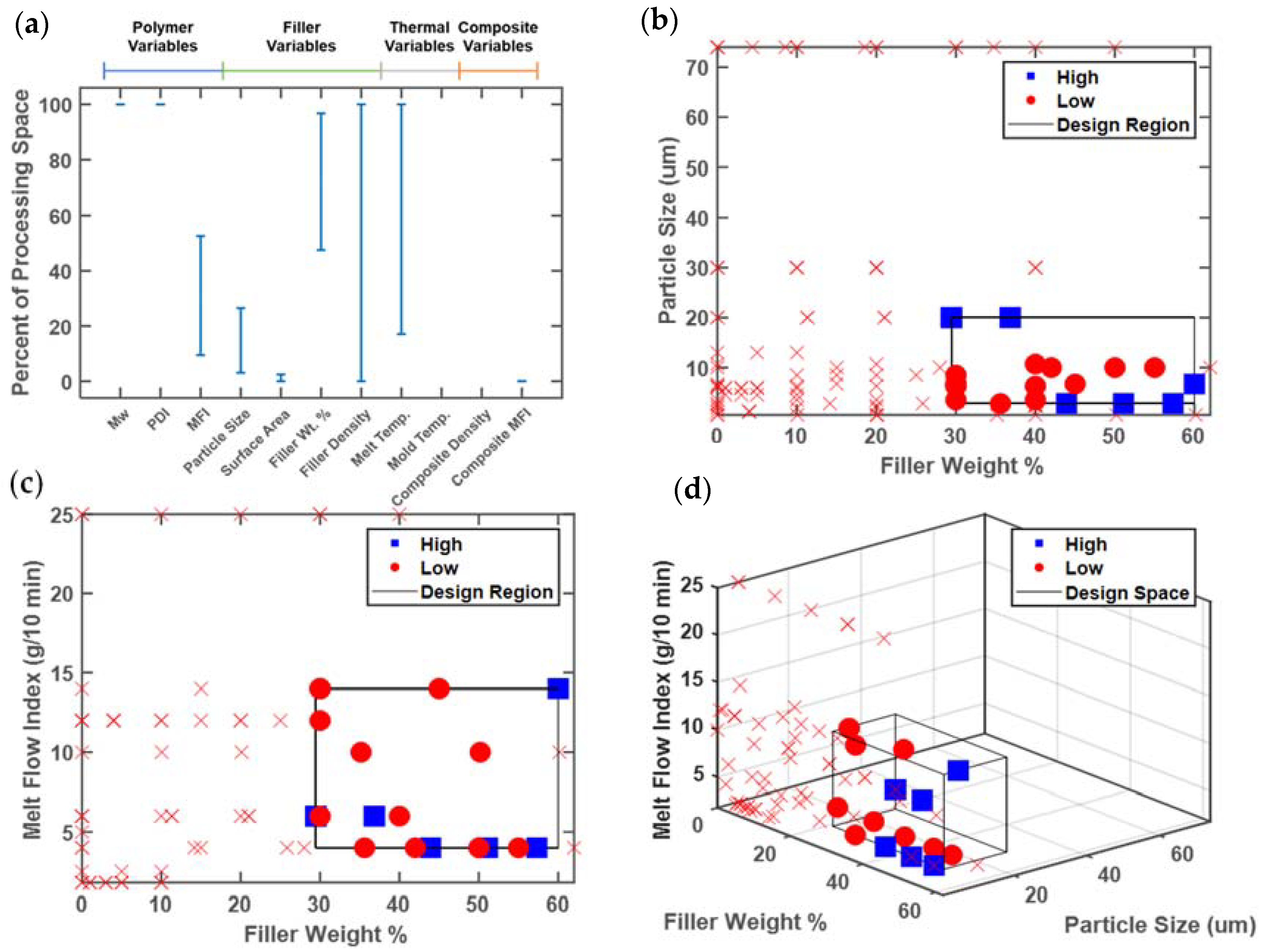
Similar to the P3HT study, the minimum and maximum reported values of 11 continuous design variables were identified in the full database and the high-performing subset to calculate rs. The results of this one-dimensional analysis are shown in Figure 6a, using variables scaled to the minimum and maximum values in the database. Several design variables have an extremely limited range of values associated with high performance, namely, polymer weight-average molecular weight, polymer polydispersity, filler surface area, and composite density. In all four cases, this large reduction in range is due to very low rates of reporting. For example, only 30 data points have the molecular weight reported, and only two of those points have a ‘high’ performance. Both data points are from the same publication and have the same molecular weight. Other design variables have no range reported at all, including mold temperature and composite melt flow index (MFI), again due to underreporting—none of the high performing points have values for mold temperature or composite MFI.
In contrast, filler density and melt temperature are reported for most entries. Since the only filler in the database is talc, there is little actual variation in its reported density, except for one outlier entry that may be misreported [28]. The melt temperature also extends across most of the range in the database, although low values (lowest 20% of the reported range) seem to be undesirable since they are never reported together with a ‘high’ performance.
The design variables with intermediate ranges in Figure 6a are polymer MFI, filler particle size, and filler weight percent. These three design variables contribute the most information to the future experimental design. It is notable that all three are related to material composition, rather than processing conditions. The melt flow index correlates inversely with the molecular weight, but is much more commonly reported in the database, because of the difficulty of dissolving polypropylene for the characterization of molecular weight by size exclusion chromatography [51]. The database analysis suggests that high stiffness requires a low polymer MFI, or equivalently, a high molecular weight. The filler particle size must fall in the lowest third of the reported values, while the filler weight percent must fall within the upper half of the values reported in the database.
The data can also be viewed in higher-dimensional spaces, as follows: Figure 6b illustrates the promising design region associated with filler size and weight percent. Note here that original variable scales are used, rather than the scaled variable ranges of Figure 6a. Future experiments can focus on this smaller box having low (but not too low) filler size and high filler weight %. The unexplored region of particle size in the range 35–70 μm could also be tested, depending on the experimental budget and availability of larger talc particles. Figure 6c again shows a two-dimensional representation, with polymer MFI and filler weight %. The promising design region contains low values of MFI, although there is little data available at higher MFIs. Future experiments could attempt to expand this region into higher MFI values (lower molecular weight), which would also lower viscosity and thus ease processing.
The calculated metrics, including the relative area of the new design region, are shown in Table 2. Similar volumetric reductions (rs) in the identified design region are observed for the PP–talc database compared to the P3HT study. However, similar values of data reduction in the design region (Fs) for the PP–talc database suggests that the community has more thoroughly sampled the entire design region compared with the P3HT community. This could arise from the reduced number of considered design variables for the polymer composites (14 variables) compared with P3HT for organic electronics (29 variables).
Finally, a three-dimensional representation is shown in Figure 6d. The promising design region is about 5% of the volume of the full range of design variables reported in the database. Also notable in Figure 6d is the lack of data points at the high particle size of 74 μm, which were previously plotted in Figure 6b [52]. Since no value of polymer MFI was reported for those points, they cannot be visualized in Figure 6d, and more importantly, they cannot be reproduced since the value of the polymer MFI that was used is unknown. Since Gafur et al. did report the weight-average molecular weight, a model could potentially be used to estimate the unreported MFI [51,52]. Physically-based correlations provide a potential route to filling in missing data, which may be more effective than linear imputation when the relationships between design variables are known and are nonlinear, such as the inverse correlation between MFI and weight-average molecular weight (Mw). However, since the Gafur et al. data points have a ‘low’ performance, such modeling would not change the promising region.
The polypropylene–talc database contains 11 continuous design variables, but also incorporates three categorical variables, namely compatibilizer, talc surface treatment, and the film formation method. Only 23 data points report a compatibilizer with none of these data points resulting in ‘high’ performance. Twenty-two data points report a surface treatment, but only aminopropyl-trimethoxysilane (4 data points) resulted in Young’s modulus values above 5 GPa. This categorical variable presents a seldom-used processing condition to further explore. Films are formed either through extrusion or compression molding, but only compression molding produced a ‘high’ performance. Better understanding of the mechanistic reasons for improved performance via compression molding could help identify new processing conditions, but in the short term, compression molding is the preferred technique.
4. Discussion
Significant advances have been made in applying materials informatics and machine learning techniques to leverage the combined knowledge of research communities. The advent of large centralized materials data repositories that are publicly accessible has been a tremendous boon to accelerated materials discovery and process optimization. However, the curation and use of materials data that are generated on a day-to-day basis, within a given material system under a formalized materials informatics lens, is still in its infancy. Smaller, more specific databases relevant to a particular application will be required to rapidly provide chemical compositions and optimized processing conditions.
A key challenge seldom addressed in ‘small data’ materials research is how to extract meaningful process–structure relationships to target desired properties. Small data can be curated in two main approaches, namely (1) controlled experiments via the design of experiments or high-throughput methods within a single laboratory, and/or (2) mining the literature to leverage experiments conducted by the community. The former datasets are often well-structured, allowing process–property information extraction via material informatics and/or machine learning methodologies [9,11]. The latter approach involves a significantly wider scope of potential design variables, resulting in an unstructured database rife with missing and noisy data. Missing data limits the applicability of materials informatics approaches, including decisions tress, neural networks, and support vector machines. Instead, we have proposed an approach that uses all available data in a small material database to identify promising design regions for future experimentation. This approach aims to provide quantitative guidance to focus experimental work based on the collective work on the community. Ideally, these future experiments will fully characterize all design variables to enable regression and machine learning approaches. The metrics, rs and Fr have been proposed to describe the relative importance of process variable combinations in determining material performance. Design regions with smaller rs and Fr values should be prioritized for future experiments. Overall, the analysis presented is general and can be expanded to examine any subset of relevant design variables.
Several opportunities and obstacles still await the widespread use of literature-guided materials databases. Once the database has been reduced to a targeted design region that contains the ‘high’ performing data points, justifications for the presence of ‘low’ data points in this region can be suggested. In the polypropylene-talc case study, the three-dimensional promising region contains six high performing points, but also nine points with a low performance. Attempts to classify based on additional design parameters were unsuccessful. The impact factor of the journal was added as an additional classifier, which did separate the three studies containing high performance from the three studies containing low performance. With a more complex database, the incorporation of additional variables has the potential to distinguish and inform more reliable and robust datasets. A potentially problematic subset of data, termed ‘hierarchical data’, is prominent amongst materials literature. Hierarchical data is defined here as paired categorial and numerical data, in which the numerical data is only relevant for that category. An example from the P3HT case study is the spin rate that is only relevant to spin cast P3HT devices, rather than dip coated devices, which are quantified instead by the dip rate. Hierarchical data requires special attention to ensure that the numerical data is not used as a predictor without the associated categorical variables.
The most significant of challenges is the handling of missing data to ensure quality predictors that reflect all of the relevant publications and not just the most-well characterized. As discussed, mining data from highly exploratory work can result in unreported data from a lack of standardized reporting templates, the discovery of new important promising conditions and/or access to various equipment and characterization techniques. Data imputation techniques have been recently developed to fill in missing values. These techniques range in complexity from imputing the population mean value to modified nonlinear iterative partial least squares regression. The latter approach has been shown to be an effective technique when the missing data is randomly distributed, rather than in structured blocks [53]. Research by Nelson et al. and Ferrer et al. has shown that principal component analysis approaches are better suited to structured blocks of missing data that may be more prevalent when developing literature databases [54,55]. Data imputation has been applied to materials datasets but, to our knowledge, not been used on literature databases. For example, Verpoort et al. trained an artificial neural network to identify erroneous values and impute missing data based on polymer composite properties provided by manufacturers’ datasheets [56]. However, only eight out of thousands of data points were missing and imputed, a marked difference to the amount of missing data found in the literature databases. Secondary approaches to handle missing data involve physical models, where known data serves as the input to an established model to predict the missing values. In the talc case study, experimental data relating polymer molecular weight to MFI was highlighted as an example [51]. Relating the spin rate to predict missing film thickness values could serve as an example for the P3HT case study. However, accurate physical based models may require additional experiments for validation.
The development of a material database from literature data is still largely a manual process, with numerous decisions made by the curator [8]. Data must be extracted from text, tables, and graphs, and must be organized in a meaningful manner. At present, automated data extraction tools are in their infancy and their implementation presents a major technological hurdle to researchers not well-versed in machine learning. Manually extracted data will be instrumental in providing training sets for the development of such tools. In pursuit of this goal, it is essential that ontologies and schema remain flexible. Research data does not necessarily cluster into fields with hard boundaries, and as such, the entries from one field’s database should be adaptable to other fields’ databases.
Finally, experimental databases are dynamic, living documents that should be easily accessible to the community. To fully utilize an experimental database, new experiments must be added, and the analysis needs to be updated on a continual basis. The question of who curates and maintains material databases is still an ongoing question in the materials community. Kalidindi et al. suggested the National Laboratories as a central entity to create a standardized strategy for materials data analysis, but this may only be appropriate in the case of big data [1]. The Protein Databank demonstrates a different model with an independent consortium as the curating body [57]. As small dynamic experimental databases are essentially quantified in literature reviews, the responsibility may rest on individual research groups to compile data for review articles, and on publishers for long term curation.
Supplementary Materials
The following are available online at https://www.mdpi.com/2227-9717/6/7/79/s1, Talc-Database.xlsx and P3HT-Database.xlsx.
Author Contributions
Conceptualization, M.M. and M.A.G.; methodology, M.M. and M.A.G.; formal analysis, M.M.; data curation, M.M. and N.P.; writing (original draft preparation), M.M. and M.A.G.; writing (review and editing), N.P. and E.R.; funding acquisition, E.R. and M.A.G.
Funding
This research was funded by financial support from Konica Minolta.
Acknowledgments
The authors thank Carson Meredith, Guoyan Zhang, Zihao Li, Jun Amano, and Leiming Wang for helpful discussions on the polypropylene–talc case study.
Conflicts of Interest
The authors declare no conflict of interest.
References
- Kalidindi, S.R.; De Graef, M. Materials data science: Current status and future outlook. Annu. Rev. Mater. Res. 2015, 45, 171–193. [Google Scholar] [CrossRef]
- Citrine Informatics. Available online: http://www.citrination.com (accessed on 7 June 2018).
- Calphad (Computer Coupling of Phase Diagrams and Thermochemistry). Available online: http://www.calphad.org (accessed on 7 June 2018).
- The Materials Project. Available online: http://www.materialsproject.org (accessed on 7 June 2018).
- Open Quantum Materials Database. Available online: http://oqmd.org (accessed on 7 June 2018).
- Nist (National Institute of Standards and Technology) Data Gateway. Available online: http://srdata.nist.gov/gateway/gateway?dblist=1 (accessed on 7 June 2018).
- Casciato, M.J.; Vastola, J.T.; Lu, J.C.; Hess, D.W.; Grover, M.A. Initial experimental design methodology incorporating expert conjecture, prior data, and engineering models for deposition of iridium nanoparticles in supercritical carbon dioxide. Ind. Eng. Chem. Res. 2013, 52, 9645–9653. [Google Scholar] [CrossRef]
- Kim, E.; Huang, K.; Saunders, A.; McCallum, A.; Ceder, G.; Olivetti, E. Materials synthesis insights from scientific literature via text extraction and machine learning. Chem. Mater. 2017, 29, 9436–9444. [Google Scholar] [CrossRef]
- Agrawal, A.; Deshpande, P.; Cecen, A.; Basavarsu, G.; Choudhary, A.; Kalidindi, S. Exploration of data science techniques to predict fatigue strength of steel from composition and processing parameters. Integr. Mater. Manuf. Innov. 2014, 3, 1–19. [Google Scholar] [CrossRef]
- Matnavi Nims Materials Database. Available online: http://mits.nims.go.jp/index_en.html (accessed on 7 June 2018).
- Ren, F.; Ward, L.; Williams, T.; Laws, K.J.; Wolverton, C.; Hattrick-Simpers, J.; Mehta, A. Accelerated discovery of metallic glasses through iteration of machine learning and high-throughput experiments. Sci. Adv. 2018, 4, 1–11. [Google Scholar] [CrossRef] [PubMed]
- AbuOmar, O.; Nouranian, S.; King, R.; Bouvard, J.L.; Toghiani, H.; Lacy, T.E.; Pittman, C.U. Data mining and knowledge discovery in materials science and engineering: A polymer nanocomposites case study. Adv. Eng. Inform. 2013, 27, 615–624. [Google Scholar] [CrossRef]
- Zhang, S.L.; Zhang, Z.X.; Xin, Z.X.; Pal, K.; Kim, J.K. Prediction of mechanical properties of polypropylene/waste ground rubber tire powder treated by bitumen composites via uniform design and artificial neural networks. Mater. Des. 2010, 31, 1900–1905. [Google Scholar] [CrossRef]
- Ling, J.; Hutchinson, M.; Antono, E.; Paradiso, S.; Meredig, B. High-dimensional materials and process optimization using data-driven experimental design with well-calibrated uncertainty estimates. Integr. Mater. Manuf. Innov. 2017, 6, 207–217. [Google Scholar] [CrossRef]
- Park, J.; Howe, J.D.; Sholl, D.S. How reproducible are isotherm measurements in metal–organic frameworks? Chem. Mater. 2017, 29, 10487–10495. [Google Scholar] [CrossRef]
- Persson, N.; McBride, M.; Grover, M.; Reichmanis, E. Silicon valley meets the ivory tower: Searchable data repositories for experimental nanomaterials research. Curr. Opin. Solid State Mater. Sci. 2016, 20, 338–343. [Google Scholar] [CrossRef]
- Box, G.E.; Wilson, K.B. On the experimental attainment of optimum conditions. J. R. Stat. Soc. 1951, 13, 1–45. [Google Scholar]
- Montgomery, D.C. Design and Analysis of Experiments, 7th ed.; Wiley: New York, NY, USA, 2009. [Google Scholar]
- Kim, S.; Kim, H.; Lu, J.-C.; Casciato, M.J.; Grover, M.A.; Hess, D.W.; Lu, R.W.; Wang, X. Layers of experiments with adaptive combined design. Nav. Res. Logist. 2015, 62, 127–142. [Google Scholar] [CrossRef]
- Dimitrakopoulos, C.D.; Malenfant, P.R.L. Organic thin film transistors for large area electronics. Adv. Mater. 2002, 14, 99–117. [Google Scholar] [CrossRef]
- Persson, N.E.; Chu, P.H.; McBride, M.; Grover, M.; Reichmanis, E. Nucleation, growth, and alignment of poly(3-hexylthiophene) nanofibers for high-performance ofets. Acc. Chem. Res. 2017, 50, 932–942. [Google Scholar] [CrossRef] [PubMed]
- Persson, N.; McBride, M.; Grover, M.; Reichmanis, E. Automated analysis of orientational order in images of fibrillar materials. Chem. Mater. 2016, 29, 3–14. [Google Scholar] [CrossRef]
- Persson, N.E.; Rafshoon, J.; Naghshpour, K.; Fast, T.; Chu, P.H.; McBride, M.; Risteen, B.; Grover, M.; Reichmanis, E. High-throughput image analysis of fibrillar materials: A case study on polymer nanofiber packing, alignment, and defects in organic field effect transistors. ACS Appl. Mater. Interfaces 2017, 9, 36090–36102. [Google Scholar] [CrossRef] [PubMed]
- Shubhra, Q.T.H.; Alam, A.; Quaiyyum, M.A. Mechanical properties of polypropylene composites. J. Thermoplast. Compos. Mater. 2011, 26, 362–391. [Google Scholar] [CrossRef]
- Ahmed, S.; Jones, F.R. A review of particulate reinforcement theories for polymer composites. J. Mater. Sci. 1990, 25, 4933–4942. [Google Scholar] [CrossRef]
- Paul, D.R.; Robeson, L.M. Polymer nanotechnology: Nanocomposites. Polymer 2008, 49, 3187–3204. [Google Scholar] [CrossRef]
- Samuels, R.J. Polymer structure: The key to process-property control. Polym. Eng. Sci. 1985, 25, 864–874. [Google Scholar] [CrossRef]
- Premalal, H.; Ismail, H.; Baharin, A. Comparison of the mechanical properties of rice husk powder filled polypropylene composites with talc filled polypropylene composites. Polym. Test. 2002, 21, 833–839. [Google Scholar] [CrossRef]
- Pukanszky, B.; Belina, K.; Rockenbauer, A.; Maurer, R.H.J. Effect of nucleation, filler anisotropy and orientation on the properties of pp composities. Composites 1993, 3, 205–214. [Google Scholar]
- Rivnay, J.; Mannsfeld, S.C.; Miller, C.E.; Salleo, A.; Toney, M.F. Quantitative determination of organic semiconductor microstructure from the molecular to device scale. Chem. Rev. 2012, 112, 5488–5519. [Google Scholar] [CrossRef] [PubMed]
- Arias, A.C.; MacKenziew, J.D.; McCulloch, I.; Rivnay, J.; Salleo, A. Materials and applications for large area electronics: Solution-based approaches. Chem. Rev. 2010, 110, 3–24. [Google Scholar] [CrossRef] [PubMed]
- Sirringhaus, H.; Brown, P.J.; Friend, R.H.; Nielsen, M.; Bechgaard, K.; Langeveld-Voss, B.; Spiering, A.; Janssen, R.; Meijer, E.; Herwig, P.; et al. Two-dimensional charge transport in self-organized, high-mobility conjugated polymers. Nature 1999, 401, 685–688. [Google Scholar] [CrossRef]
- Kline, R.; McGehee, M.; Kadnikova, E.; Liu, J.; Frechet, J.; Toney, M.F. Dependence of regioregular poly(3-hexylthiophene) film morphology and field-effect mobility on molecular weight. Macromolecules 2005, 38, 3312–3319. [Google Scholar] [CrossRef]
- Bronstein, H.A.; Luscombe, C.K. Externally initiated regioregular p3ht with controlled molecular weight and narrow polydispersity. J. Am. Chem. Soc. 2009, 131, 12894–12895. [Google Scholar] [CrossRef] [PubMed]
- Horowitz, G. Organic field effect transistors. Adv. Mater. 1998, 10, 365–377. [Google Scholar] [CrossRef]
- Choi, D.; Chu, P.-H.; McBride, M.; Reichmanis, E. Best practices for reporting organic field effect transistor device performance. Chem. Mater. 2015, 27, 4167–4168. [Google Scholar] [CrossRef]
- Raccuglia, P.; Elbert, K.C.; Adler, P.D.; Falk, C.; Wenny, M.B.; Mollo, A.; Zeller, M.; Friedler, S.A.; Schrier, J.; Norquist, A.J. Machine-learning-assisted materials discovery using failed experiments. Nature 2016, 533, 73–76. [Google Scholar] [CrossRef] [PubMed]
- Kline, R.; McGehee, M.; Kadnikova, E.; Liu, J.; Frechet, J. Controlling the field-effect mobility of regioregular polythiophene by changing the molecular weight. Adv. Mater. 2003, 15, 1519–1522. [Google Scholar] [CrossRef]
- Zen, A.; Pfaum, J.; Hirschmann, S.; Zhuang, W.; Jaiser, F.; Asawapirom, U.; Rabe, J.; Scherf, U.; Neher, D. Effect of molecular weight and annealing of poly(3-hexylthiophene)s on the performance or organic field-effect transistors. Adv. Funct. Mater. 2004, 14. [Google Scholar] [CrossRef]
- Himmelberger, S.; Vandewal, K.; Fei, Z.; Heeney, M.; Salleo, A. Role of molecular weight distribution on charge transport in semiconducting polymers. Macromolecules 2014, 47, 7151–7157. [Google Scholar] [CrossRef]
- Scharsich, C.; Lohwasser, R.; Sommer, M.; Asawapirom, U.; Scherf, U.; Thelakkat, M.; Neher, D.; Köhler, A. Control of aggregate formation in poly(3-hexylthiophene) by solvent, molecular weight, and synthetic method. J. Polym. Sci. Part B Polym. Phys. 2012, 50, 442–453. [Google Scholar] [CrossRef]
- Chang, M.; Lim, G.; Park, B.; Reichmanis, E. Control of molecular ordering, alignment, and charge transport in solution-processed conjugated polymer thin films. Polymers 2017, 9, 212. [Google Scholar] [CrossRef]
- Chang, M.; Choi, D.; Fu, B.; Reichmanis, E. Solvent based hydrogen bonding: Impact on poly(3-hexylthiophene) nanoscale morphology and charge transport characteristics. ACS Nano 2013, 7, 5402–5413. [Google Scholar] [CrossRef] [PubMed]
- Roesing, M.; Howell, J.; Boucher, D. Solubility characteristics of poly(3-hexylthiophene). J. Polym. Sci. Part B Polym. Phys. 2017. [Google Scholar] [CrossRef]
- Choi, D.; Chang, M.; Reichmanis, E. Controlled assembly of poly(3-hexylthiophene): Managing the disorder to order transition on the nano- through meso-scales. Adv. Funct. Mater. 2015, 25, 920–927. [Google Scholar] [CrossRef]
- Verilhac, J.; LeBlevennec, G.; Djurado, D.; Rieutord, F.; Chouiki, M.; Travers, J.; Pron, A. Effect of macromolecular parameters and processing conditions on supramolecular organisation, morphology and electrical transport properties in thin layers of regioregular poly(3-hexylthiophene). Synth. Met. 2006, 156, 815–823. [Google Scholar] [CrossRef]
- Joshi, S.; Grigorian, S.; Pietsch, U.; Pingel, P.; Zen, A.; Neher, D.; Scherf, U. Thickness dependence of the crystalline structure and hole mobility in thin films of low molecular weight poly(3-hexylthiophene). Macromolecules 2008, 41, 6800–6808. [Google Scholar] [CrossRef]
- Na, J.Y.; Kang, B.; Sin, D.H.; Cho, K.; Park, Y.D. Understanding solidification of polythiophene thin films during spin-coating: Effects of spin-coating time and processing additives. Sci. Rep. 2015, 5, 13288. [Google Scholar] [CrossRef] [PubMed]
- Chu, P.H.; Kleinhenz, N.; Persson, N.; McBride, M.; Hernandez, J.; Fu, B.; Zhang, G.; Reichmanis, E. Toward precision control of nanofiber orientation in conjugated polymer thin films: Impact on charge transport. Chem. Mater. 2016, 28, 9099–9109. [Google Scholar] [CrossRef]
- Chang, M.; Choi, D.; Egap, E. Macroscopic alignment of one-dimensional conjugated polymer nanocrystallites for high-mobility organic field-effect transistors. ACS Appl. Mater. Interfaces 2016, 8, 13484–13491. [Google Scholar] [CrossRef] [PubMed]
- Bermner, T.; Rudin, A. Melt flow index values and molecular weight distributions of commercial thermoplastics. J. Appl. Polym. Sci. 1990, 41, 1617–1627. [Google Scholar] [CrossRef]
- Gafur, M.A.; Nasrin, R.; Mina, M.F.; Bhuiyan, M.A.H.; Tamba, Y.; Asano, T. Structures and properties of the compression-molded istactic-polypropylene/talc composites: Effect of cooling and rolling. Polym. Degrad. Stab. 2010, 95, 1818–1825. [Google Scholar] [CrossRef]
- Nelson, P.R.C. Treatment of Missing Measurements in PCA and PLS Models. Ph.D. Thesis, Master University, Hamilton, ON, Canada, 2002. [Google Scholar]
- Nelson, P.R.C.; Taylor, P.A.; MacGregor, J.F. Missing data methods in pca and pls: Score calculations with incomplete observations. Chemom. Intell. Lab. Syst. 1996, 35, 45–65. [Google Scholar] [CrossRef]
- Folch-Fortuny, A.; Arteaga, F.; Ferrer, A. Pca model building with missing data: New proposals and a comparative study. Chemom. Intell. Lab. Syst. 2015, 146, 77–88. [Google Scholar] [CrossRef]
- Verpoort, P.C.; MacDonald, P.; Conduit, G.J. Materials data validation and imputation with an artificial neural network. Comput. Mater. Sci. 2018, 147, 176–185. [Google Scholar] [CrossRef] [Green Version]
- Berman, H.M.; Westbrook, J.; Feng, Z.; Gilliland, G.; Bhat, T.N.; Weissig, H.; Shindyalov, I.N.; Bourne, P.E. The Protein Data Bank. Available online: https://www.rcsb.org/ (accessed on 7 June 2018).
Figure 1.
Flow chart of classification approach to constructed reduced design regions.

Figure 2.
One possible processing route for poly-3-hexylthiophene (P3HT), and a key property of interest in organic field-effect transistor (OFET) performance.
Figure 2.
One possible processing route for poly-3-hexylthiophene (P3HT), and a key property of interest in organic field-effect transistor (OFET) performance.

Figure 3.
Proposed polymer and filler to develop high strength composites and a key property of interest: Young’s modulus.
Figure 3.
Proposed polymer and filler to develop high strength composites and a key property of interest: Young’s modulus.

Figure 4.
Representative analysis plots of (a) one-, (b) two-, and (c) three-dimensional classifying design variables, resulting in charge mobility values exceeding 0.1 cm2/V·s. Blue squares are data points above the cutoff, red dots represent points below the cutoff but within the target design region, and red x markers indicate all other data points below the cutoff but not within the target region. All axis ranges denote the full range of values present in the database.

Figure 5.
Illustrative two-dimensional plots indicating (a) limited collective screening of the entire design region (sparsity), and (b) inconsistent reporting and characterization. Axis values denote the full range of values present in the database.
Figure 5.
Illustrative two-dimensional plots indicating (a) limited collective screening of the entire design region (sparsity), and (b) inconsistent reporting and characterization. Axis values denote the full range of values present in the database.

Figure 6.
Representative analysis plots of (a) one-, (b,c) two-, and (d) three-dimensional analysis, classifying design variables that result in Young’s modulus exceeding 5 GPa. All axis values denote the full range of values present in the database. Blue squares are data points above the cutoff, red dots represent points below the cutoff but within the target design region, and the red x markers indicate all other data points below the cutoff but not within the target design region.


Table 1.
Metrics for the two-dimensional analysis of the poly-3-hexylthiophene (P3HT) system. PDI—polymer polydispersity index, RR—polymer regioregularity.
Table 1.
Metrics for the two-dimensional analysis of the poly-3-hexylthiophene (P3HT) system. PDI—polymer polydispersity index, RR—polymer regioregularity.
| PDI/Hansen Radius | PDI/Film Thickness | Hansen Radius/Film Thickness | Channel Length/Annealing Temp | RR/Film Thickness | |
|---|---|---|---|---|---|
| rs (%) | 27 | 12 | 10 | 25 | 4 |
| Fr (%) | 45 | 30 | 53 | 45 | 63 |
Table 2.
Quantified metrics of two-dimensional analysis for the PP–talc system. MFI—melt flow index.
Table 2.
Quantified metrics of two-dimensional analysis for the PP–talc system. MFI—melt flow index.
| MFI/Particle Size | MFI/Filler Wt.% | Particle Size/Filler Wt.% | |
|---|---|---|---|
| rs (%) | 10 | 21 | 12 |
| Fr (%) | 28 | 14 | 15 |
© 2018 by the authors. Licensee MDPI, Basel, Switzerland. This article is an open access article distributed under the terms and conditions of the Creative Commons Attribution (CC BY) license (http://creativecommons.org/licenses/by/4.0/).
Share and Cite
MDPI and ACS Style
McBride, M.; Persson, N.; Reichmanis, E.; Grover, M.A. Solving Materials’ Small Data Problem with Dynamic Experimental Databases. Processes 2018, 6, 79. https://doi.org/10.3390/pr6070079
AMA Style
McBride M, Persson N, Reichmanis E, Grover MA. Solving Materials’ Small Data Problem with Dynamic Experimental Databases. Processes. 2018; 6(7):79. https://doi.org/10.3390/pr6070079
Chicago/Turabian StyleMcBride, Michael, Nils Persson, Elsa Reichmanis, and Martha A. Grover. 2018. "Solving Materials’ Small Data Problem with Dynamic Experimental Databases" Processes 6, no. 7: 79. https://doi.org/10.3390/pr6070079
Note that from the first issue of 2016, this journal uses article numbers instead of page numbers. See further details here.