The Role of Immune Response in Optimal HIV Treatment Interventions

Abstract

A mathematical model for the transmission dynamics of human immunodeficiency virus (HIV) within a host is developed. Our model focuses on the roles of immune response cells or cytotoxic lymphocytes (CTLs). The model includes active and inactive cytotoxic immune cells. The basic reproduction number and the global stability of the virus free equilibrium is carried out. The model is modified to include anti-retroviral treatment interventions and the controlled reproduction number is explored. Their effects on the HIV infection dynamics are investigated. Two different disease stage scenarios are assessed: early-stage and advanced-stage of the disease. Furthermore, optimal control theory is employed to enhance healthy CD4${}^{+}$ T cells, active cytotoxic immune cells and minimize the total cost of anti-retroviral treatment interventions. Two different anti-retroviral treatment interventions (RTI and PI) are incorporated. The results highlight the key roles of cytotoxic immune response in the HIV infection dynamics and corresponding optimal treatment strategies. It turns out that the combined control (both RTI and PI) and stronger immune response is the best intervention to maximize healthy CD4${}^{+}$ T cells at a minimal cost of treatments.

1. Introduction

Human immunodeficiency virus (HIV) is the pathogen responsible for one of the world’s most lethal diseases, acquired immune deficiency syndrome (AIDS). The pathogen attacks the immune system in a human body, particularly, CD4${}^{+}$ T cells, which help the immune system fight off infections and disease. Untreated HIV can destroy CD4${}^{+}$ T cells and an infected person can be exposed to many opportunistic diseases [1,2]. When HIV invades the body, it targets the CD4${}^{+}$ T cells where the viral RNA is converted into viral DNA, thus producing more viral particles. CD4${}^{+}$ T cells are responsible for sending signals to the immune system such as cytotoxic cells (cytotoxic lymphocytes (CTL), CD8 T cells and natural killer cells). Then, cytotoxic cells respond to this message and set out to kill infected cells by lysing infected cells, causing them to explode. Thus, cytotoxic cells can remove infected cells from the the body and inhibit viral replication, but they do not directly kill free viruses. Over time, HIV is able to deplete the population of CD4${}^{+}$ T cells, preventing that cytotoxic cells from being deployed. CD4${}^{+}$ T cells count in a healthy person is about 1000 mm${}^{-3}$, when the cell count reaches 200 mm${}^{-3}$ or below in a HIV-patient, and some opportunistic diseases arises, then the person is classified as having AIDS [3,4].

World health institutions provide different combinations of medicines and treatments that lead to mitigate symptoms and reduce susceptibility to opportunistic diseases, increasing life quality and expectancy. It is difficult to establish the kind of treatment and its intensity, due to the conditions related to the virus, a patient (as immunological conditions) and social and economical issues in each country [5]. Anti-retroviral guidelines have established the primary goal of antiretroviral treatment (ART) as the reduction of the HIV-associated morbidity and mortality in 2011 [6]. The guideline recommends drug treatments for patients with CD4${}^{+}$ T cells between 350–500 cells/mm${}^3$ and as optional when it is over 500 cells/mm${}^3$. Reverse transcriptase inhibitors (RTI)-based therapy inhibits reverse transcription by being incorporated into the newly synthesized viral DNA and thus preventing its further elongation, or by directly binding to the enzyme and interfering with its function. On the other hand, protease inhibitors (PI)-based therapy causes infected cells to produce non-infectious virions (virions created prior to drug treatment remain infectious) [7].

There have been remarkable attentions on the HIV dynamics among scientists in medicine and mathematical biology. Significant efforts have been made in order to understand and to characterize the underlying mechanism of the disease. Particularly, the mathematical framework has been employed to model the transmission dynamics of HIV/AIDS [8,9,10,11,12]. Earlier mathematical models have considered HIV/AIDS dynamics within a host using delay differential equations [13,14,15,16,17] and some models have focused on the viral and CD4${}^{+}$ T cell dynamics [18,19]. Recently, there has been some work to explore the impact of the immune response in the HIV dynamics [20,21,22]. Furthermore, mathematical models have incorporated explicitly the effect of the immune response and their results have been analyzed and investigated [3,4,23]. In relation to the immune responses, studies suggest to take into account the possibility of small or no immune response in some situations and a strong response in others. No matter which approach is considered, research has suggested that treatment strategies must incorporate RTI and PI, which leads to a therapy based on drug cocktails of multiple treatments taken in combination [24]. Indeed, the fact that HIV replicates rapidly (producing ${10}^{10}$ viral particles per day) shows that HIV infection progresses too fast to be treated under a single drug treatment [7,24]. Recent research has shown that the benefits of RTI and PI drugs can be reduced by the development of drug resistance [25,26]. This process of accelerated replication leads to the genetic variability of the virus and a high degree of genetic variability can quickly generate drug-resistant variants in response to the therapy. The evolution of an HIV patient is influenced by several factors such as lifestyle, current immune system state, drug resistance, other health conditions as well as the economic capability to afford an efficient medical treatment. Hence, when a drug treatment is recommended to a patient, these aspects should be taken into account.

The aim of this paper is twofold. First, a SIR-type mathematical model is used to investigate the roles of cytotoxic immune response (CTL) in HIV dynamics within a host, as proposed in [27]. The SIR-type model is a compartmental model using a system of nonlinear ordinary differential equations. The model consists of three compartments—S for the number susceptible, I for the number of infectious, and R for the number recovered. Cytotoxic cells are divided into two compartments, corresponding to inactive and active cytotoxic cells, which prevent the extinction of cytotoxic immune cells in the absence of HIV. The basic reproduction number $R_0$ is computed, then we establish the global stability of the virus free equilibrium (VFE). Secondly, the model is modified to include RTI and PI treatment interventions to determine the effectiveness needed to mitigate the infection. Moreover, due to a time-varying evolution of the disease, time-varying treatments should be scheduled as well [3,4,28]. Drugs can be costly and can be harmful when high dosages are given. Therefore, an optimal control problem is formulated to highlight the importance of a high level of CD4${}^{+}$ T cells and strong active immune response while minimizing the cost of treatments.

2. A HIV Model with Immune Responses

A mathematical model for HIV dynamics within a host has been proposed in our previous work [27]. First, T and $T^{*}$ are the average concentration of healthy CD4${}^{+}$ T cells and infected CD4${}^{+}$ T cells, respectively. Further, M and $M^{*}$ are the average concentration of inactive and active cytotoxic cells, respectively. Lastly, V is the average concentration of viral particles (viral load). Hence, the model can be written as the following nonlinear ordinary differential equations:

$$\left\{\begin{array}{c}\dot{T}=\sigma -\beta TV-\mu T\hfill \\ {\dot{T}}^{*}=\beta TV-\gamma T^{*}{M}^{*}-\delta T^{*}\hfill \\ \dot{M}=\lambda -\psi T^{*}M-\rho M\hfill \\ {\dot{M}}^{*}=\alpha T^{*}{M}^{*}+\psi T^{*}M-\rho M^{*}\hfill \\ \dot{V}=\eta T^{*}-cV,\hfill \end{array}\right.$$

(1)

where $\sigma$ denotes the constant recruitment of healthy cells from the thymus and bone marrow. It is assumed that a healthy T cell becomes infected through effective contact with an infected virus V at a constant rate $\beta$. Parameter $\delta$ denotes the natural death rate of healthy CD4${}^{+}$ T cells. The active immune cells $M^{*}$ kill infected cells by the rate $\gamma T^{*}{M}^{*}$. $\alpha$ is the active cytotoxic cells replication rate and $\alpha T^{*}{M}^{*}$ denotes the average of new active cytotoxic cells by replication. Under the assumption $\gamma \ge \alpha$, immune cells kill more than they replicate themselves by this process.

The inactive immune response is produced by the body at a constant rate $\lambda$; considering that infected cells stimulate the inactive immune cells at a rate $\psi$, an average of $\psi T^{*}M$ inactive immune cells become active. The natural death rate of both inactive and active immune cells is denoted by $\rho$. Viral particles are replicated by infected cells during their lifespan. This viral replication is usually proportional to the number of dead infected cells $\delta T^{*}$. Hence, a viral replication term can be described as $\eta T^{*}=N\delta T^{*}$, where N is an average number of viruses produced by cells lysis (note that $\eta =N\delta$). The natural death rate of virus is c and the loss of viral particles during infection is neglected, as in [2,7,27,29]. The description of parameters is collected in

Table 1. Parameter definitions and baseline values (and their corresponding sources) used in numerical simulations.

	Description	Early-Stage	Advanced-Stage	Ref.
$\sigma$	Source term for uninfected CD4${}^{+}$ T cells	10 mm${}^3·$d${}^{-1}$	10 mm${}^3·$d${}^{-1}$	[3,23]
$\beta$	Rate CD4 T${}^{+}$ cell becomes infected by virus	$2.5\times {10}^{-5}$ mm${}^3·$d${}^{-1}$	$2.5\times {10}^{-5}$ mm${}^3·$d${}^{-1}$	[23]
$\mu$	Death rate of uninfected CD4${}^{+}$ T cells	$1\times {10}^{-2}$ d${}^{-1}$	$1\times {10}^{-2}$ d${}^{-1}$	[3]
$\delta$	Death rate of infected CD4${}^{+}$ T cells	0.26 d${}^{-1}$	0.26 d${}^{-1}$	[3,23]
N	Number of viruses produced by cells lysis	500	500	[3]
c	Death rate of virus	2.4 d${}^{-1}$	2.4 d${}^{-1}$	[23]
$\psi$	Rate of immune response activation	$2\times {10}^{-3}$ mm${}^3·$d${}^{-1}$	$2\times {10}^{-2}$ mm${}^3·$d${}^{-1}$	-
$\alpha$	Rate of immune response proliferation	$5\times {10}^{-5}$ mm${}^3·$d${}^{-1}$	$5\times {10}^{-4}$ mm${}^3·$d${}^{-1}$	[23]
$\rho$	Death rate of immune response	0.1 mm${}^3·$d${}^{-1}$	0.1 mm${}^3·$d${}^{-1}$	[3,23]
$\gamma$	Rate infected cells killed by CTL	$2\times {10}^{-3}$ mm${}^{-3}·$d${}^{-1}$	$4\times {10}^{-3}$ mm${}^{-3}·$d${}^{-1}$	[23]
$\lambda$	Source term for immune response	5 mm${}^3·$d${}^{-1}$	5 mm${}^3·$d${}^{-1}$	[23]
b	Upper bound for RTI and PI effectiveness	1	1	[23]
$T_0$	Initial value for uninfected CD4${}^{+}$ T cells	1000	500	[23]
$T_0^{*}$	Initial value for infected CD4${}^{+}$ T cells	0	350	[23]
$M_0$	Initial value for non-active mmune cells	0	25	[23]
$M_0^{*}$	Initial value for active mmune cells	1	20	[23]
$V_0$	Initial value for virus	$1\times {10}^{-3}$	$2.5\times {10}^4$	[23]

.

2.1. The Basic Reproduction Number and Stability Analysis

Theorem 1.

If $\gamma \ge \alpha$, the set $\mathsf{\Omega }=\left\{(C,V)\in {\mathbb{R}}_{+}^5|T\le \frac{\sigma }{\mu };T+T^{*}+M+M^{*}\le \frac{\sigma +\lambda }{\epsilon };V\le \frac{\eta (\sigma +\lambda )}{c\epsilon }\right\}$ is a positively invariant set for the system (1).

Proof. 

The dynamics of healthy cells satisfies $\dot{T}\le \sigma -\mu T$; hence, it is true that ${\displaystyle \underset{t\to +\infty }{lim\; sup}}T\le \frac{\sigma }{\mu }$. Similarly, ${\displaystyle \underset{t\to +\infty }{lim\; sup}}C\le \frac{\sigma +\lambda }{\epsilon }$, where $C=T+T^{*}+M+M^{*}$ and $\epsilon =max\{\mu ,\delta ,\rho \}$; finally, ${\displaystyle \underset{t\to +\infty }{lim\; sup}}V\le \frac{\eta (\sigma +\lambda )}{c\epsilon }$. Hence, the set:

$$\mathsf{\Omega }=\left\{(T,T^{*},M,M^{*},V)\in {\mathbb{R}}_{+}^5|T\le \frac{\sigma }{\mu };T+T^{*}+M+M^{*}\le \frac{\sigma +\lambda }{\epsilon };V\le \frac{\eta (\sigma +\lambda )}{c\epsilon }\right\}$$

is a compact, attractive positively invariant set for the system (1) if $\gamma \ge \alpha$. Hence, all solutions of the system (1) with positive initial conditions remain positive and bounded. □

The virus free equilibrium (VFE) of the system (1) is given by $E_0=({\overline{T}}_0,0,{\overline{M}}_0,0,0)$, where ${\overline{T}}_0=\frac{\sigma }{\mu }$ and ${\overline{M}}_0=\frac{\lambda }{\rho }$, which always belong to $\mathsf{\Omega }$. The basic reproduction number is calculated by using the methodology (the next generation matrix approach) outlined in [30,31]. Now, we let $F\left(x\right)$ represent the rate of appearance of new infections. The net transition rates out of the corresponding compartment are represented by $V\left(x\right)$. Then, we find the Jacobian matrix of $F\left(\mathbf{x}\right)$ and $V\left(\mathbf{x}\right)$ (denoting $\mathcal{F}=\left[\frac{\partial F}{\partial {\mathbf{x}}_j}\right]$ and $\mathcal{V}=\left[\frac{\partial V}{\partial {\mathbf{x}}_j}\right]$) and evaluate it at the virus free equilibrium of the system (1) is given by $E_0=({\overline{T}}_0,0,{\overline{M}}_0,0,0)$ with ${\overline{T}}_0=\frac{\sigma }{\mu }$ and ${\overline{M}}_0=\frac{\lambda }{\rho }$, which

$$\mathcal{F}=\left[\begin{array}{ccccc}0& 0& 0& 0& 0\\ 0& 0& 0& 0& \beta {\overline{T}}_0\\ 0& 0& 0& 0& 0\\ 0& \psi {\overline{M}}_0& 0& 0& 0\\ 0& 0& 0& 0& 0\end{array}\right],\mathcal{V}=\left[\begin{array}{ccccc}\mu & 0& 0& 0& \beta {\overline{T}}_0\\ 0& \delta & 0& 0& 0\\ 0& \psi {\overline{M}}_0& \rho & 0& 0\\ 0& 0& 0& -\rho & 0\\ 0& -\eta & 0& 0& c\end{array}\right].$$

(2)

The spectral radius of the matrix ${\mathcal{FV}}^{-1}$ can give the basic reproduction number as

$$R_0=\frac{\eta }{\delta }\frac{\beta {\overline{T}}_0}{c}.$$

(3)

Recall that $R_0$ means the number of secondary cases on average produced by one infected cell during its lifespan in a completely susceptible population. An infected cell produces $\frac{\eta }{\delta }$ viral particles during its lifespan. These viral particles infect $\frac{\eta \beta }{\delta c}{\overline{T}}_0$ T cells during their lifespan. This dimensionless quantity is a key concept in mathematical epidemiology. In fact, it determines whether the disease (virus) dies out (when $R_0<1$) or persists (when $R_0>1$).

Theorem 2.

The virus free equilibrium is globally asymptotically stable if $R_0\le 1$.

Proof. 

Let us consider the Lyapunov functional, $L=T^{*}+\frac{\delta }{\eta }V$. Then, the derivative of L along the trajectories of the system can be written as

$$\begin{array}{ccc}\hfill \dot{L}& =& \beta TV-\gamma T^{*}{M}^{*}-\delta T^{*}+\frac{\delta }{\eta }\left(\eta T^{*}-cV\right)\hfill \\ & =& \frac{\delta c}{\eta }\left(\frac{\beta \eta }{\delta c}T-1\right)V-\gamma T^{*}{M}^{*}\hfill \\ & =& \frac{\delta c}{\eta }\left(\frac{R_0}{T_0}T-1\right)V-\gamma T^{*}{M}^{*}\hfill \\ & \le & \frac{\delta c}{\eta }(R_0-1)V\le 0.\hfill \end{array}$$

If $\dot{L}=0$, then $\left(\frac{\beta \eta }{\delta c}T-1\right)V=0$ and $T^{*}{M}^{*}=0$. Hence, the largest invariant set included in $\{\dot{L}=0\}$ is reduced to the virus free equilibrium. Thus, by LaSalle’s invariance principle [32,33], the VFE is globally asymptotically stable. □

2.2. An HIV Model with Constant ART Interventions

In this section, the model (1) is modified to include ART based on the application of reverse transcriptase inhibitors (RTI) and protease inhibitors (PI) as the primary strategies to reduce the number of new infections. Drug efficiency is represented by the controls $u_1$ and $u_2$, which account respectively for reverse transcriptase (RTI) and protease inhibitor (PI) actions. Assume that $u_1$ and $u_2$ are constant valued functions, where $u_i\in [0,1]$ for $i=1,2$ ($u_i=0$ means no drug and $u_i=1$ means 100% effective). By introducing these constant treatments into the model (1), we obtain the following system:

$$\left\{\begin{array}{c}\dot{T}=\sigma -\beta (1-u_1)TV-\mu T\hfill \\ {\dot{T}}^{*}=\beta (1-u_1)TV-\gamma T^{*}{M}^{*}-\delta T^{*}\hfill \\ \dot{M}=\lambda -\psi T^{*}M-\rho M\hfill \\ {\dot{M}}^{*}=\alpha T^{*}{M}^{*}-\rho M^{*}+\psi T^{*}M\hfill \\ \dot{V}=\eta (1-u_2)T^{*}-cV\hfill \\ \dot{W}=\eta u_2{T}^{*}-cW.\hfill \end{array}\right.$$

(4)

Here, $W=W\left(t\right)$ represents the average concentration of non-infectious viral particles at time t. The terms $\eta (1-u_2)T^{*}$ and $\eta u_2{T}^{*}$ should be interpreted as the average number of infectious and non-infectious viral particles produced per infected cell, respectively.

For the new model (4), the basic reproduction number with controls (treatments), denoted by $R_c$, is calculated by using the next generation method, given as:

$$R_c(u_1,u_2)=\frac{\beta (1-u_1)\eta (1-u_2){\overline{T}}_0}{\delta c}.$$

(5)

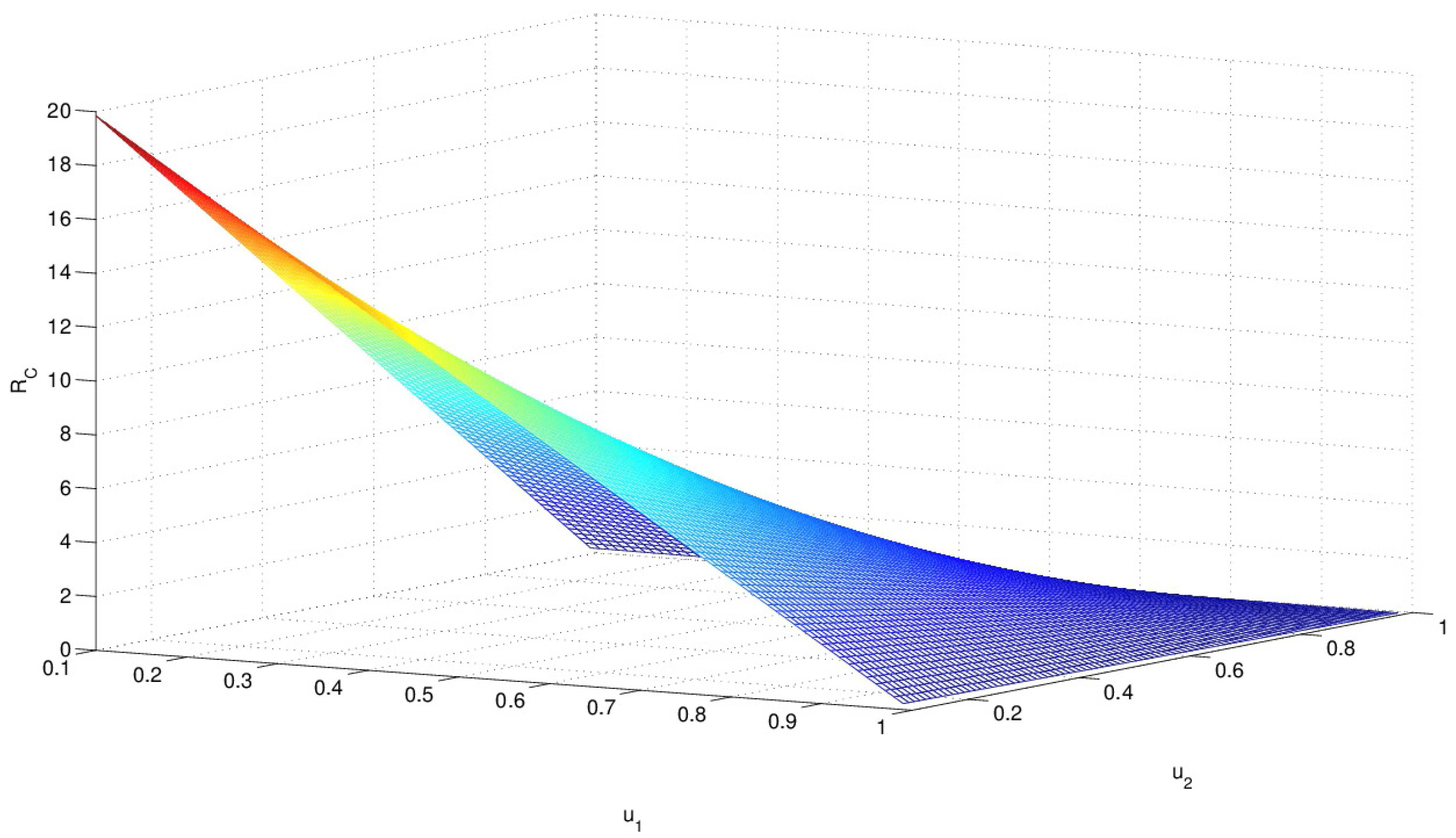
Please note that $R_c$ is a function of the controls $u_1$ and $u_2$, as shown in Figure 1. $R_c(u_1,u_2)$ monotonely decreases as both controls $u_1$ and $u_2$ approach to 1. When two controls are near zero, $R_c$ gets very large and in such a case, HIV infection is almost uncontrollable. Hence, it is ideal to have a higher level of both controls ($u_1$ and $u_2$ near 1).

Based on the stability analysis of system (1), it can be proven that $R_c\le 1$ guarantees VFE is globally asymptotically stable. The aim is to find control thresholds $u_1^c$ and $u_2^c$ that guarantee the infection dies out; i.e., threshold values of $u_1$ and $u_2$ that ensure $R_c<1$. In case of RTI treatment only, $0\le u_1\le 1$ and $u_2=0$, and expression (5) takes the form:

$$R_c\left(u_1\right)=\frac{\beta (1-u_1)\eta {\overline{T}}_0}{\delta c}.$$

From the condition $R_c<1$, and using the expression for $R_0$ given in (3), we find the threshold for RTI intervention is given by

$$u_1>\frac{R_0-1}{R_0}=u_1^c.$$

(6)

This expression makes sense only if $R_0>1$ (a necessary condition to have long-term infection). Therefore, theoretically, the infection could be eliminated from the body when the effectiveness of RTI satisfies the above condition (6).

Similarly, we find that the threshold for PI treatment only, that is $u_1=0$ and $0\le u_2\le 1$, is given by,

$$u_2>\frac{R_0-1}{R_0}=u_2^c.$$

(7)

Again, when $R_0>1$, the infection persists. The infection could be eliminated from the body when the effectiveness of PI satisfies the above condition (7).

3. Optimal Control Formulation

In this section, an optimal control problem is formulated to highlight the importance of a high concentration level of CD4${}^{+}$ T-cells and strong active immune response to minimize the cost of treatments. Specifically, the goal is to determine optimal control functions $u_1\left(t\right)$ and $u_2\left(t\right)$ that maximize the number of healthy CD4${}^{+}$ T-cells and the active immune response at a minimal treatment cost. Therefore, the objective functional is given by

$$J(u_1\left(t\right),u_2\left(t\right))={\int }_0^{\tau }\left(w_{1}T\left(t\right)+w_2{M}^{*}\left(t\right)-\frac{A}{2}{u}_1^2\left(t\right)-\frac{B}{2}{u}_2^2\left(t\right)\right)dt,$$

(8)

where $w_1$ and $w_2$ are weight (or balance) constants on the infected hosts and vectors, respectively. The weight constants A and B are the relative costs of the implementation of $u_1$ (RTI) and $u_2$ (PI), respectively. We model the control efforts as a linear combination of quadratic terms, $u_i^2\left(t\right)$ ($i=1,2$), due to the convexity of the controls in the objective functional. Now, the goal is to obtain an optimal pair ($\tilde{U}$, $\tilde{X}$) such that

$$J\left(\tilde{U}\right)=max\left\{J\left(U\right)\right|U\in \mathsf{\Gamma }\},$$

(9)

where

$$\mathsf{\Gamma }=\left\{(u_1\left(t\right),u_2\left(t\right))\in {\left(L^1\left([0,\tau ]\right)\right)}^2|0\le u_1\left(t\right),u_2\left(t\right)\le b,t\in [0,\tau ]\right\}.$$

In other words, we want to maximize the functional J over $\mathsf{\Gamma }$ subject to the state system (4) with $U=(u_1,u_2)$ and $X=(T\left(t\right),T^{*}\left(t\right),M\left(t\right),M^{*}\left(t\right),V\left(t\right),W\left(t\right))$. The existence of optimal controls is guaranteed from standard results on optimal control theory. Pontryagin’s Maximum Principle is used to establish necessary conditions that must be satisfied by an optimal solution [34]. This leads to the following theorem.

Theorem 3.

Given the optimal control $\tilde{U}\left(t\right)\in \mathsf{\Gamma }$ and the optimal solution $(\tilde{T},{\tilde{T}}^{*},\tilde{M},{\tilde{M}}^{*},\tilde{V},\tilde{W})$ from the state system (4), there exist adjoint functions ${\varphi }_i$ ($i=$ 1, ⋯, 6) satisfying the following system of differential equations,

$$\left\{\begin{array}{c}\frac{d{\varphi }_1}{dt}=-(w_1-{\varphi }_1\beta (1-u_1)V+{\varphi }_2\beta (1-u_1)V-\mu {\varphi }_1)\hfill \\ \frac{d{\varphi }_2}{dt}=-(-{\varphi }_2\gamma M^{*}-{\varphi }_2\delta +{\varphi }_3\psi M+{\varphi }_4\alpha M+{\varphi }_4\psi M+{\varphi }_5\eta (1-u_2)+{\varphi }_6\eta u_2)\hfill \\ \frac{d{\varphi }_3}{dt}=-({\varphi }_3\psi T^{*}-{\varphi }_3\rho +{\varphi }_4\psi T^{*})\hfill \\ \frac{d{\varphi }_4}{dt}=-(w_2-{\varphi }_2\gamma T^{*}+{\varphi }_4\alpha T^{*}-{\varphi }_4\rho )\hfill \\ \frac{d{\varphi }_5}{dt}=-(-{\varphi }_1\beta (1-u_1)T+{\varphi }_2\beta (1-u_1)T-{\varphi }_{5}c)\hfill \\ \frac{d{\varphi }_6}{dt}=c{\varphi }_6\hfill \end{array}\right.$$

(10)

subject to the transversality condition ${\varphi }_i\left(\tau \right)=0$, for i = 1,…,6, where

$${\tilde{u}}_1=max\left(0,min\left(\frac{\beta TV({\varphi }_1-{\varphi }_2)}{A},b\right)\right)\mathrm{and}{\tilde{u}}_2=max\left(0,min\left(\frac{\eta T^{*}({\varphi }_6-{\varphi }_5)}{B},b\right)\right).$$

(11)

Proof. 

The Hamiltonian system is defined as

$$\begin{array}{cc}H\hfill & =w_{1}T+w_2{M}^{*}-\frac{A}{2}{u}_1^2-\frac{B}{2}{u}_2^2+{\varphi }_1(\sigma -\beta (1-u_1)TV-\mu T)\hfill \\ & +{\varphi }_2(\beta (1-u_1)TV-\gamma T^{*}{M}^{*}-\delta T^{*})\hfill \\ & +{\varphi }_3(\lambda -\psi T^{*}M-\rho M)+{\varphi }_4(\alpha T^{*}{M}^{*}-\rho M^{*}+\psi T^{*}M)\hfill \\ & +{\varphi }_5(\eta (1-u_2)T^{*}-cV)+{\varphi }_6(\eta u_2{T}^{*}-cW)\hfill \\ & +z_1{u}_1+z_2(b-u_1)+z_3{u}_2+z_4(b-u_2)\hfill \end{array}$$

where $z_i$ for $i=1,\dots ,4$ are non-negative penalty multipliers for $0\le u_1\left(t\right),u_2\left(t\right)\le b$ such that

$$z_1{u}_1=0,z_2(b-u_1)=0,z_3{u}_2=0,z_4(b-u_2)=0.$$

(12)

The Hamiltonian H is maximized with respect to the controls, so we differentiate H with respect to $u_i$ on the set $\mathsf{\Gamma }$, respectively. Hence, we obtain the following optimality conditions, $\frac{\partial H}{\partial u_1}=0$ and $\frac{\partial H}{\partial u_2}=0$:

$$u_1=\frac{\beta TV({\varphi }_1-{\varphi }_2)-z_1+z_2}{A}\mathrm{and}{u}_2=\frac{\eta T^{*}({\varphi }_6-{\varphi }_5)-z_3+z_4}{B}$$

The next step is to use the penalty functions $z_i$ for $i=1,\dots ,4$ and (12) to determine the bounded controls for ${\tilde{u}}_1$ and ${\tilde{u}}_2$.

In the case $0<u_1,u_2<b$, we have $z_1=z_2=z_3=z_4=0$, thus

$${\tilde{u}}_1=\frac{\beta TV({\varphi }_1-{\varphi }_2)}{A}\mathrm{and}{\tilde{u}}_2=\frac{\eta T^{*}({\varphi }_6-{\varphi }_5)}{B}.$$

If $u_1=0$ and $u_2=0$ then $z_1\ge 0$, $z_2=0$, $z_3\ge 0$ and $z_4=0$, and so

$$0=\frac{\beta TV({\varphi }_1-{\varphi }_2)}{A}-\frac{z_1}{A}\mathrm{and}0=\frac{\eta T^{*}({\varphi }_6-{\varphi }_5)}{B}-\frac{z_3}{B}.$$

It is evident from the last two expressions that $\frac{\beta TV({\varphi }_1-{\varphi }_2)}{A}\ge 0$ and $\frac{\eta T^{*}({\varphi }_6-{\varphi }_5)}{B}\ge 0$. Hence,

$${\tilde{u}}_1=min\left(\frac{\beta TV({\varphi }_1-{\varphi }_2)}{A},b\right)\mathrm{and}{\tilde{u}}_2=min\left(\frac{\eta T^{*}({\varphi }_6-{\varphi }_5)}{B},b\right).$$

Finally, if $u_1=b$ and $u_2=b$, we have $z_1=0$, $z_2\ge 0$, $z_3=0$ and $z_4\ge 0$, so

$$b=\frac{\beta TV({\varphi }_1-{\varphi }_2)}{A}+\frac{z_2}{A}\mathrm{and}b=\frac{\eta T^{*}({\varphi }_6-{\varphi }_5)}{B}+\frac{z_4}{B}.$$

Hence, $\frac{\beta TV({\varphi }_1-{\varphi }_2)}{A}\le b$ and $\frac{\eta T^{*}({\varphi }_6-{\varphi }_5)}{B}\le b$. Now in order to guarantee those expressions are greater than 0, we have the following

$${\tilde{u}}_1=max\left(0,\frac{\beta TV({\varphi }_1-{\varphi }_2)}{A}\right)\mathrm{and}{\tilde{u}}_2=max\left(0,\frac{\eta T^{*}({\varphi }_6-{\varphi }_5)}{B}\right)$$

We obtain the following optimality conditions by unifying all the arguments above for the bounded controls $0\le u_i\left(t\right)\le b$ for $i=1,2$:

$${\tilde{u}}_1=max\left(0,min\left(\frac{\beta TV({\varphi }_1-{\varphi }_2)}{A},b\right)\right)\mathrm{and}{\tilde{u}}_2=max\left(0,min\left(\frac{\eta T^{*}({\varphi }_6-{\varphi }_5)}{B},b\right)\right).$$

(13)

Next, the existence of optimal controls follows since the integrand of J is a convex function of $U\left(t\right)$ and the the state system satisfies the $Lipschitz$ property with respect to the state variables [35]. The following can be derived from Pontryagin’s Maximum Principle [34]:

$$\begin{array}{ccccc}{\displaystyle \frac{d{\varphi }_1}{dt}}=-{\displaystyle \frac{\partial H}{\partial T}}\hfill & \hfill & {\displaystyle \frac{d{\varphi }_2}{dt}}=-{\displaystyle \frac{\partial H}{\partial T^{*}}}\hfill & \hfill & {\displaystyle \frac{d{\varphi }_3}{dt}}=-{\displaystyle \frac{\partial H}{\varphi M}}\hfill \\ {\displaystyle \frac{d{\varphi }_4}{dt}}=-{\displaystyle \frac{\varphi H}{\partial M^{*}}}\hfill & \hfill & {\displaystyle \frac{d{\varphi }_5}{dt}}=-{\displaystyle \frac{\partial H}{\partial V}}\hfill & \hfill & {\displaystyle \frac{d{\varphi }_6}{dt}}=-{\displaystyle \frac{\partial H}{\partial W}},\hfill \end{array}$$

where

$$\left\{\begin{array}{c}\frac{d{\varphi }_1}{dt}=-(w_1-{\varphi }_1\beta (1-u_1)V+{\varphi }_2\beta (1-u_1)V-\mu {\varphi }_1)\hfill \\ \frac{d{\varphi }_2}{dt}=-(-{\varphi }_2\gamma M^{*}-{\varphi }_2\delta +{\varphi }_3\psi M+{\varphi }_4\alpha M+{\varphi }_4\psi M+{\varphi }_5\eta (1-u_2)+{\varphi }_6\eta u_2)\hfill \\ \frac{d{\varphi }_3}{dt}=-({\varphi }_3\psi T^{*}-{\varphi }_3\rho +{\varphi }_4\psi T^{*})\hfill \\ \frac{d{\varphi }_4}{dt}=-(w_2-{\varphi }_2\gamma T^{*}+{\varphi }_4\alpha T^{*}-{\varphi }_4\rho )\hfill \\ \frac{d{\varphi }_5}{dt}=-(-{\varphi }_1\beta (1-u_1)T+{\varphi }_2\beta (1-u_1)T-{\varphi }_{5}c)\hfill \\ \frac{d{\varphi }_6}{dt}=c{\varphi }_6\hfill \end{array}\right.$$

(14)

subject to the transversality condition ${\varphi }_i\left(\tau \right)=0$, for $i=1,\dots ,6$, and evaluated at the optimal controls and corresponding states, which results in the adjoint system given above. □

The above optimality system is a two-point boundary value problem. This problem can be solved by the following process, first, the state system (4) is solved with initial conditions using an initial guess for the control. Secondly, the adjoint system (14) is solved with transversality conditions. Then, the controls are updated in each iteration using formula (13) for optimal controls. Last, the iterations continue until the predefined convergence criteria is achieved.

4. Numerical Simulations

4.1. Numerical Simulations in the Absence of Interventions

In this section, we present numerical simulations by solving the system (1) in the absence of treatments (or controls). Particularly, we are interested in two scenarios incorporating the level of disease progress in the HIV transmission dynamics. The first is an early-stage case for an average patient who just became infected. For an initial healthy T cell population at early-stage, $T\left(0\right)=1000$ cells/mm${}^3$ is used. The second is an advanced-stage corresponding to a patient who became infected some time ago. Hence, for the advanced-stage, an initial condition of the healthy T cell population is set to be half of the early stage one, $T\left(0\right)=500$ cells/mm${}^3$. Other initial conditions for the advanced-stage have been estimated from simulations (as shown in Table 1).

Also, these cases can be characterized by how successfully the immune response can destroy infected cells; this leads to changes in parameters $\alpha$, $\psi$ and $\gamma$. Therefore, parameter values for $\alpha$, $\psi$, $\gamma$ as well as initial conditions are varied to simulate the early-stage and the advanced-stage scenarios. Parameter values for the immune cells have been taken from [3,23], except that $\psi$ that is used ad hoc. Once the organism is attacked by the infected virus, the cytotoxic immune response begins maintaining an effort to keep the immune system at a normal condition, leading to an increase in $\alpha$ and $\psi$. On the other hand, its capability to destroy infected cells might decrease (a reduction in $\gamma$), which is due to changes in the viral particles and their fast replication rate. Simulation time is chosen as 100-day period ($\tau =100$) since a treatment is considered as effective provided it lowers strongly viral load within two months [23]. The baseline parameter values used in these simulations are given in Table 1.

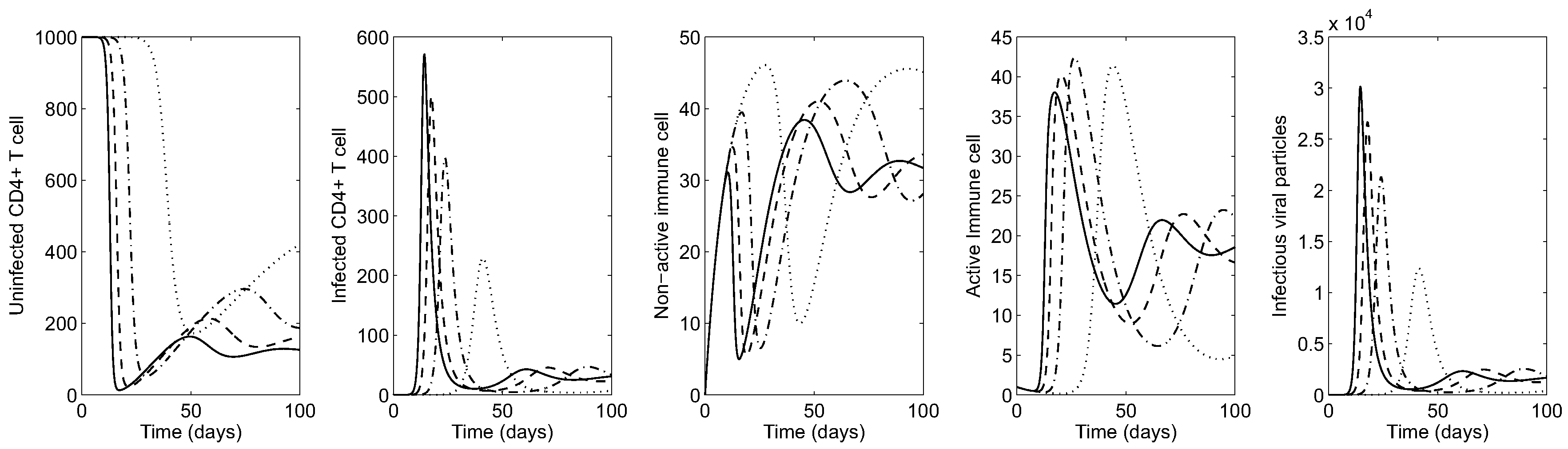
First, the impact of the transmission rate $\beta$ on the HIV dynamics is illustrated under both scenarios. Figure 2 illustrates the time series of HIV infection for an early-stage in the absence of treatments. Here it is assumed the patient has a normal count of CD4${}^{+}$ T-cells and develops infectious viral particles around $t=20$ days. The greater the probability in the transmission rate $\beta$, the greater the average of infected cells and viral particles (see the solid curve in the right most panel for the viral load, which is almost identical with infected CD4${}^{+}$ T cells). This causes a sharp decrease in the concentration of healthy CD4${}^{+}$ T-cells (see the left most panel), which becomes more pronounced under larger values of $\beta$. The organism responds by activating immune response cells, which fight against the virus in a highly nonlinear way (see the middle panels for immune cells).

Figure 3 shows the HIV dynamics for an advanced-stage case in the absence of controls. That is, a patient with a lower level of healthy CD4${}^{+}$ T-cells whose cells are already being attacked by the virus. Please note that a higher level of viral particles causes a sharp decrease in the concentration of healthy CD4${}^{+}$ T-cells within a very short time period (see the left most panel). Again, this becomes more pronounced under larger values of $\beta$. For the advanced-stage case, the organism has a stronger response by activating immune response cells in a higher level (see the middle panels for active immune cells).

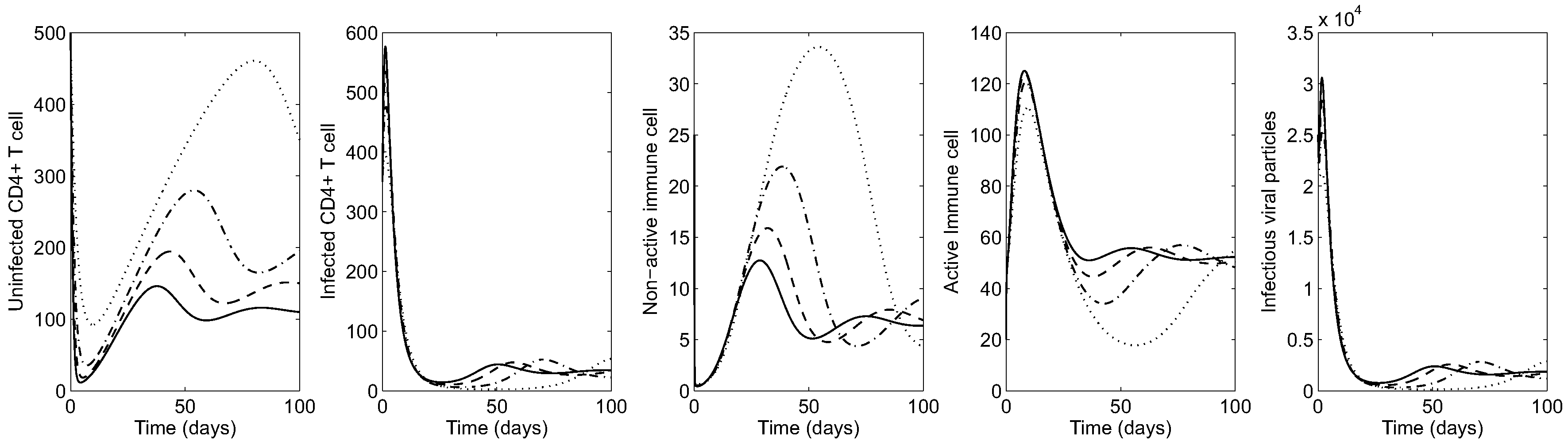
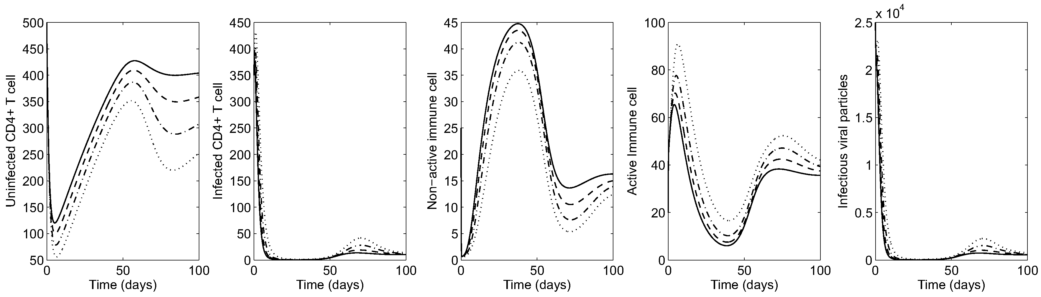
Next, the impact of cytotoxic cells on the HIV dynamics is shown by varying $\gamma$ (the rate of infected cells killed by CTL). Figure 4 illustrates the HIV dynamics in the early-stage patient. It is clear that the greater the effectiveness of cytotoxic cells in killing infected cells, the lower the average of infected cells and viral particles and the greater the average number of healthy CD4${}^{+}$ T cells. Using $\gamma =0.9$, virus and infected CD4${}^{+}$ T cells are mostly under control (see the solid curve in all panels). Under larger values of $\gamma$, the average number of active (inactive) cytotoxic cells increase (decrease), as seen in the middle panels.

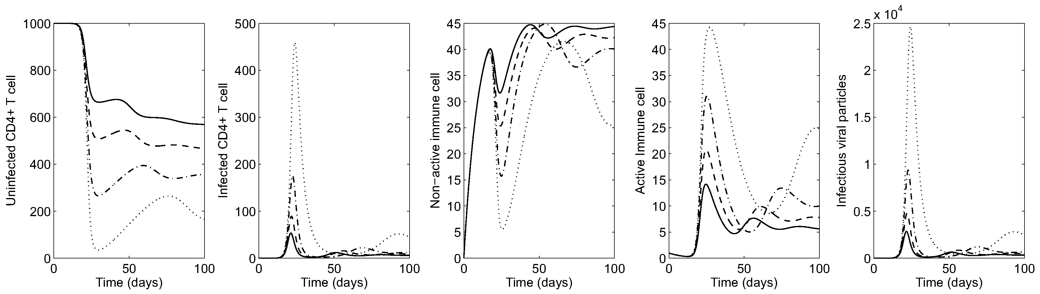
Figure 5 shows the HIV dynamics for an advanced-stage patient varying $\gamma$ to illustrate the effect of cytotoxic immune response on the evolution of infection. Similarly, it is observed that larger values of $\gamma$ lead to more uninfected CD4${}^{+}$ T-cells (over 300 cells per mm${}^3$; see the solid curve in the left most panel). Under larger values of $\gamma$, the average of active (inactive) cytotoxic cells increase (decrease) as seen in the middle panels. Even though virus and infected CD4${}^{+}$ T cells are most manageable when $\gamma =0.008$, infection cannot be eliminated from the body by cytotoxic immune cells alone.

These results highlight the roles of the immune response to intervene with the organism either to control or reduce the evolution of the disease in order to avoid deterioration of patient health. In this case, we propose implementation of optimal treatment interventions by increasing the population of healthy CD4${}^{+}$ T cells and the activation level of immune response cells. In the next section, we discuss the results with optimal treatments.

4.2. Numerical Simulations in the Presence of Optimal Treatments

In this section, we present numerical simulations by solving the optimality system described in the previous section. Again, two scenarios on the level of HIV infection progress are carried out. For both cases, we run simulations under several different values of weight constants. These weight constants are selected since the magnitude of the virus population is much larger than the magnitude of the cost of controls in the objective functional (8) (this difference in magnitude is balanced by this choice of A and B). The resulting HIV dynamics with the corresponding optimal control functions are presented in Figure 6 and Figure 7.

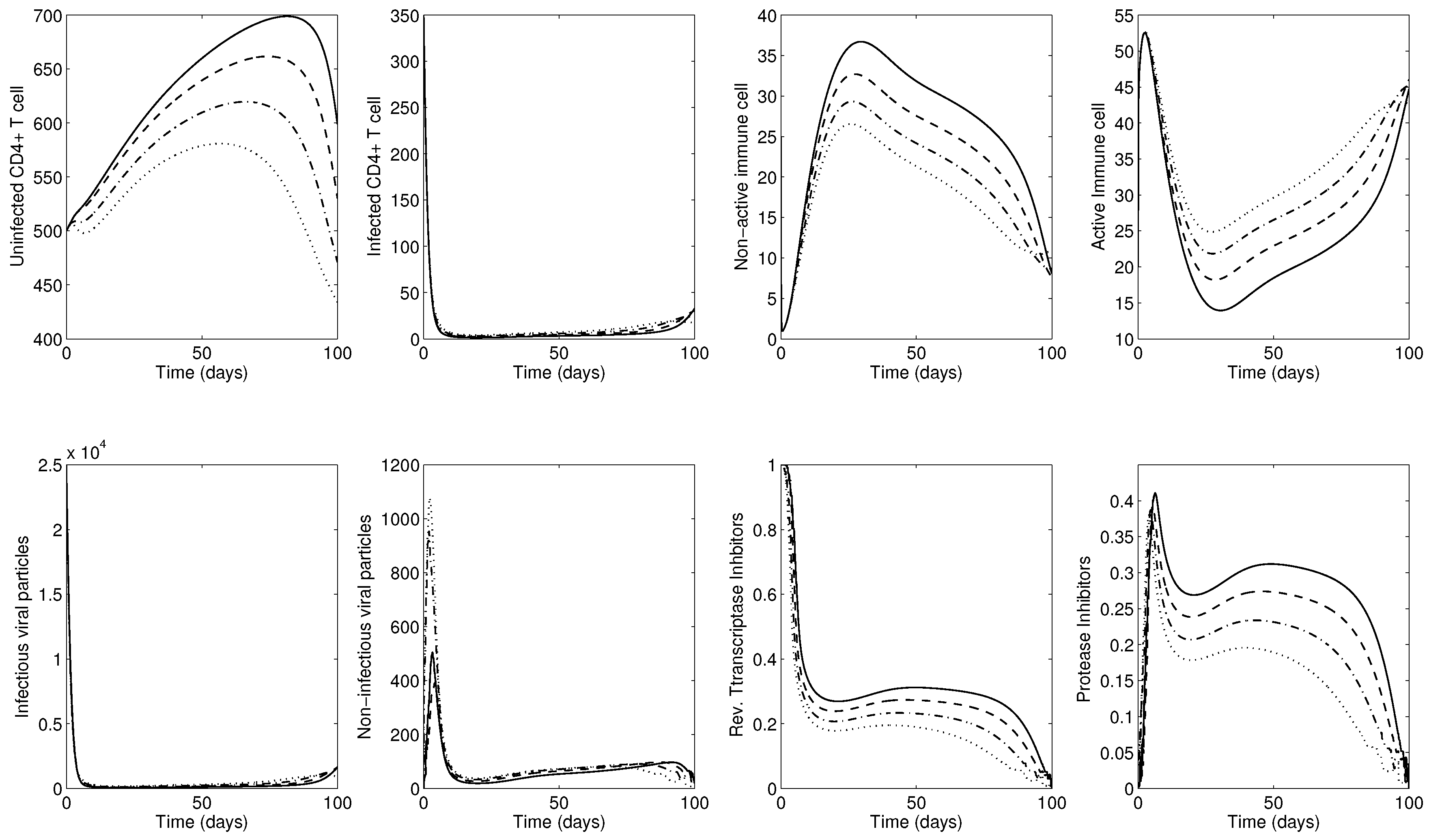
First, the results for early-stage disease are illustrated in Figure 6. Four different weight constants have been chosen to compare the impact of costs in two controls. The bottom two right panels show time-dependent optimal controls for reverse transcriptase inhibitor ($u_1$) and protease inhibitor ($u_2$). The two controls RTI ($u_1$) and PI ($u_2$) should be applied at a medium level during the entire simulation. The top leftmost panel shows the corresponding uninfected CD4${}^{+}$ T cells. Overall uninfected CD4${}^{+}$ T cells remain at a high level almost until the final time, where the two treatments are reduced to zero (no controls are given at around $t=100$, as shown in the bottom two right panels).

Under smaller values of weight constants A and B, which thereby decrease the cost of treatments, the optimal control function increases in a linear manner (monotone increases). Hence, the best treatment protocols are when $A=B=12,500$ (see the solid curves in the panels), which maintain the active immune response at a lower level. This may indicate that implementation of both treatments take control of infection, inducing a kind of laziness in the immune response. In other words, the immune system puts forth more effort to fight against infections when there are fewer treatments. Nonetheless, optimal treatment interventions (combination of RTI and PI) effectively control infection regardless of these weight constants.

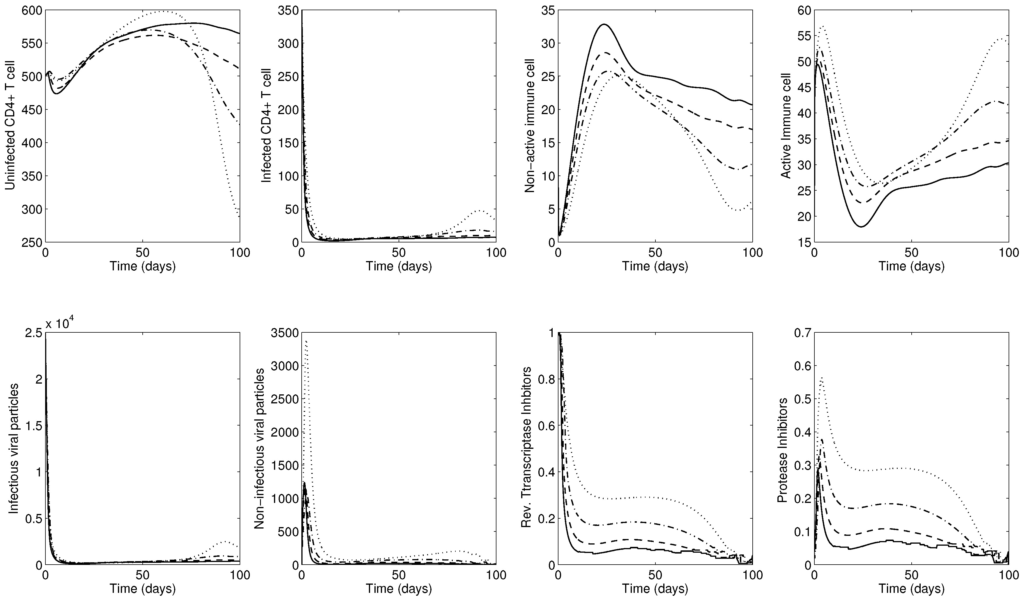
Next, Figure 7 shows the results for the advanced-stage using $\gamma =0.004$. The bottom two right panels show time-dependent optimal controls for reverse transcriptase inhibitor ($u_1$) and protease inhibitor ($u_2$). Initially, a maximum level of RTI should be implemented, followed by decreasing the RTI, while the PI should be applied at a medium level during the entire simulation. Similarly, the overall number of uninfected CD4${}^{+}$ T cells remains relatively high almost until the final time (see the top leftmost panel). Under smaller values of weight constants A and B, which thereby decrease the cost of treatments, the optimal control function is increasing in a nonlinear manner.

Please note that the most effective treatments are the case of the lowest weight constants $A=B=$ 12,500 (a greater level of healthy CD4${}^{+}$ T cells is obtained; see the solid curves in the panels). Interestingly, the use of ART increases the reservoir of inactive cytotoxic cells M, resulting in reduced activation of these cells since ART takes control of the HIV infection (see the solid curves in the top right two panels). These findings establish that the treatment does most of the hard work of inhibiting viral replication and raising the number of healthy CD4${}^{+}$ T cells, but this is counteracted by the weakened cytotoxic response of the body to fight off the infection naturally.

This phenomenon is clearer in Figure 8 using $A=B=$ 12,500 under different values of $\gamma$ to illustrate the effects of stronger cytotoxic response on the corresponding HIV dynamics and controls. The bottom two right panels show time-dependent optimal controls for reverse transcriptase inhibitor ($u_1$) and protease inhibitor ($u_2$). Under larger values of $\gamma$, both controls are decreasing and the average number of active immune cells $M^{*}$ is decreasing (see the solid curves in the top panels). Therefore, the combined control and stronger immune response is the best intervention to maximize the level of healthy CD4${}^{+}$ T cells at a minimal cost of treatments.

5. Conclusions

In this paper, we have presented an HIV transmission model by incorporating immune response and anti-retroviral (ART) interventions. The immune response has been divided into two components: active and inactive immune cells. Two different disease stages (early-stage and advanced-stage) have been assessed in our numerical simulations. Moreover, optimal control theory has been utilized to obtain optimal treatments to maximize healthy CD4${}^{+}$ T cells and active immune response at a minimal cost of treatments. The combined interventions of RTI and PI are implemented in both the early-stage and the advanced-stage scenarios.

Our results indicate that the optimal strategy succeeds in reducing infection and improves the number of CD4${}^{+}$ T cells. Also, in practice, ART by itself is strong enough to control infection and maintain a high level of healthy CD4${}^{+}$ T cells. However, combined interventions of RTI and PI have some undesirable effects of reducing the activation of cytotoxic immune response, therefore, they can interrupt the natural process of the immune system of acquiring memory against the virus.

As observed in the results of larger values of $\gamma$, both controls are decreasing and the average number of active immune cells $M^{*}$ is decreasing. Therefore, the combined control and stronger immune response is the best intervention to maximize the level of healthy CD4${}^{+}$ T cells at a minimal treatment cost. This allows the immune system to regain control over infection. Such strategies should contribute to build effective immune memory against the virus, and hence reduction of treatment costs and the side effects associated with the treatments for a longer term therapy. If the immune system is efficient (strong immune response), then it is possible to maintain the effectiveness of treatment for longer and at lower levels. This remarkable fact motivates us to carry out a new research direction, which involves the evolution of immune response cells in sub-optimal control strategies or controlled interrupted treatments. That is, treatments are given only when CD4${}^{+}$ T cells and immune cells are lower than a certain threshold.

Certainly, HIV dynamics in the presence of immune response is more complicated than the results presented by our model. It is important to consider viral mutations and the acquisition of drug resistance as critical factors that interfere with HIV dynamics and optimal treatments. Therefore, optimal antiretroviral treatment strategies can be improved with the aid of HIV resistance tests. Unfortunately, this issue is beyond the scope of this paper and it should be addressed in the future HIV research. However, the findings in this paper can exhibit some possibilities and approaches of using numerical analysis and optimal control theory to obtain a better understanding HIV dynamics with treatments. Hence, we hope to achieve new insights in the HIV infection evolution via optimal treatments in the near future.

References

- Covert, D.; Kirschner, D. Revisiting early models of the host-pathogen interactions in hiv infection. Comments Theor. Biol. 2000, 5, 383–411. [Google Scholar]
- May, R.M.; Anderson, R.M. Transmission dynamics of HIV infection. Nature 1987, 326, 137–142. [Google Scholar] [CrossRef] [PubMed]
- Culshaw, R.V.; Ruan, S.; Spiteri, R.J. Optimal hiv treatment by maximising immune response. J. Math. Biol. 2004, 48, 545–562. [Google Scholar] [CrossRef] [PubMed]
- Joshi, H.R. Optimal control of an hiv immunology model. Optim. Control Appl. Methods 2002, 23, 199–213. [Google Scholar] [CrossRef]
- Pisani, E.; Cuchi, P.; Zacarias, F.; Schwartlander, B.; Stanecki, K.; Castilho, E. HIV and AIDS in the Americas: an epidemic with many faces; Joint United Nations Programme on HIV/AIDS (UNAIDS): Geneva, Switzerland, 2000. [Google Scholar]
- Panel on Antiretroviral Guidelines for Adults and Adolescents. Guidelines for the Use of Antiretroviral Agents in HIV-1-Infected Adults and Adolescents; Department of Health and Human Services: Atlanta, GA, USA, 2011; pp. 1–66.
- Perelson, A.S.; Nelson, P.W. Mathematical analysis of HIV-1 dynamics in vivo. SIAM Rev. 1999, 41, 3–44. [Google Scholar] [CrossRef]
- Adda, P.; Dimi, J.L.; Iggidr, A.; Kamgang, J.C.; Sallet, G.; Tewa, J.J. General models of host-parasite systems. Global analysis. Discret. Contin. Dyn. Syst. Ser. B 2007, 8, 1–17. [Google Scholar]
- Kirschner, D.E.; Mehr, R.; Perelson, A.S. Role of the thymus in pediatric HIV-1 infection. J. Acquir. Immune Defic. Syndr. Hum. Retrovir. 1998, 18, 95–109. [Google Scholar] [CrossRef]
- Nowak, M.A.; May, R.M. Mathematical biology of HIV infections: Antigenic variation and diversity threshold. Math. Biosci. 1991, 106, 1–21. [Google Scholar] [CrossRef]
- Perelson, A. Modeling the interaction of the immune system with HIV. In Mathematical and Statistical Approaches to AIDS Epidemiology with HIV; Castillo-Chavez, C., Ed.; Springer: Berlin/Heidelberg, Germany, 1989; pp. 350–370. [Google Scholar]
- Perelson, A.S.; Kirschner, D.E.; De Boer, R. Dynamics of HIV infection of CD4+ T cells. Math. Biosci. 1993, 114, 81–125. [Google Scholar] [CrossRef] [Green Version]
- Culshaw, R.V.; Ruan, S. A delay-differential equation model of hiv infection of CD4 T-cells. Math. Biosci. 2000, 165, 27–39. [Google Scholar] [CrossRef]
- Iggidr, A.; Mbang, J.; Sallet, G. Stability analysis of within-host parasite models with delays. Math. Biosci. 2007, 209, 51–75. [Google Scholar] [CrossRef] [PubMed] [Green Version]
- Nelson, P.W.; Murray, J.; Perelson, A.S. A model of HIV-1 pathogenesis that includes an intracellular delay. Math. Biosci. 2000, 163, 201–215. [Google Scholar] [CrossRef]
- Nelson, P.W.; Perelson, A.S. Mathematical analysis of delay differential equation models of HIV-1 infection. Math. Biosci. 2002, 179, 73–94. [Google Scholar] [CrossRef]
- Stilianakis, N.; Schenzle, D. On the intra-host dynamics of HIV-1 infections. Math. Biosci. 2006, 199, 1–25. [Google Scholar] [CrossRef] [PubMed]
- Wodarz, D.; Lloyd, A.; Jansen, A.; Nowak, M.A. Dynamics of macrophage and t cell infection by HIV. J. Theor. Biol. 1999, 196, 101–113. [Google Scholar] [CrossRef] [PubMed]
- Wodarz, D.; Nowak, M.A. Mathematical models of hiv pathogenesis and treatment. Bioessays 1999, 24, 1178–1187. [Google Scholar] [CrossRef] [PubMed]
- Kirschner, D.; Webb, G.F.; Cloyd, M. Model of HIV-1 disease progression based on virus-induced lymph node homing and homing-induced apoptosis of CD4+ lymphocytes. J. Acquir. Immune Defic. Syndr. 2000, 24, 352–362. [Google Scholar] [CrossRef] [PubMed]
- Lui, W.M. Nonlinear oscillation in models of immune responses to persistent viruses. Theor. Popul. Biol. 1997, 52, 224–230. [Google Scholar]
- Murase, A.; Sasaki, T.; Kajiwara, T. Stability analysis of pathogen-immune interaction dynamics. J. Math. Biol. Math. 2005, 51, 247–267. [Google Scholar] [CrossRef] [PubMed]
- Orellana, J.M. Optimal drug scheduling for HIV therapy efficiency improvement. Biomed. Signal Process. Control 2011, 6, 379–386. [Google Scholar] [CrossRef]
- Adams, B.M.; Banks, H.T.; Davidian, M.; dae Kwon, H.; Tran, H.T.; Wynne, S.N.; Rosenberg, E.S. HIV dynamics: Modeling, data analysis, and optimal treatment protocols. J. Comput. Appl. Math. 2005, 184, 10–49. [Google Scholar] [CrossRef]
- Bennett, D.E.; Camacho, R.J.; Otelea, D.; Kuritzkes, D.R.; Fleury, H.; Kiuchi, M.; Heneine, W.; Kantor, R.; Jordan, M.R.; Schapiro, J.M.; et al. Drug resistance mutations for surveillance of transmitted HIV-1 drug-resistance: 2009 update. PLoS ONE 2009, 4, e4724. [Google Scholar] [CrossRef] [PubMed] [Green Version]
- Johnson, V.A.; Calvez, V.; Günthard, H.F.; Paredes, R.; Pillay, D.; Shafer, R.; Wensing, A.M.; Richman, D.D. Update of the drug resistance mutations in HIV-1. HIV Med. 2010, 18, 156–163. [Google Scholar]
- Toro-Zapata, H.D.; Caicedo-Casso, A.G.; Bichara, D.; Lee, S. Role of Active and Inactive Cytotoxic Immune Response in Human Immunodeficiency Virus Dynamics. Osong Public Health Res. Perspect. 2014, 5, 3–8. [Google Scholar] [CrossRef] [PubMed]
- Wein, L.M.; Zenios, S.A.; Nowak, M.A. Dynamic multidrug therapies for HIV: A control theoretic approach. J. Theor. Biol. 1997, 185, 15–29. [Google Scholar] [CrossRef] [PubMed]
- Nowak, M.A.; Bangham, R. Population dynamics of immune responses to persistent viruses. Science 1996, 272, 74–79. [Google Scholar] [CrossRef] [PubMed]
- Diekmann, O.; Heesterbeek, J.A.P.; Metz, J.A.J. On the definition and the computation of the basic reproduction ratio R0 in models for infectious diseases in heterogeneous populations. J. Math. Biol. 1990, 28, 365–382. [Google Scholar] [CrossRef] [PubMed]
- Van den Driessche, P.; Watmough, J. Reproduction numbers and sub-threshold endemic equilibria for compartmental models of disease transmission. Math. Biosci. 2002, 180, 29–48. [Google Scholar] [CrossRef]
- LaSalle, J. Stability theory for ordinary differential equations. J. Differ. Equ. 1968, 41, 57–65. [Google Scholar] [CrossRef]
- LaSalle, J. The Stability of Dynamical Systems; Regional Conference Series in Applied Mathematics; Society for Industrial and Applied Mathematics: Philadelphia, PA, USA, 1976. [Google Scholar]
- Pontryagin, L.; Boltyanskii, V.; Gamkrelidze, R.; Mishchenko, E. The Mathematical Theory of Optimal Processes; Wiley: Hoboken, NJ, USA, 1962. [Google Scholar]
- Fleming, W.; Rishel, R. Deterministic and Stochastic Optimal Control; Springer: New York, NY, USA, 1975. [Google Scholar]
Figure 1.
The controlled reproduction number is displayed as varying two controls with and . monotonely decreases as both controls and approach 1.
Figure 2.
Early-stage HIV dynamics in the absence of controls under four different values of ( is fixed): (dotted), (dash-dot): (dashed) and (solid).
Figure 3.
Advanced-stage HIV dynamics in the absence of controls under four different values of ( is fixed): (dotted), (dash-dot); (dashed) and (solid).
Figure 4.
Early-stage HIV dynamics in the absence of controls under four different values of ( is fixed): (dotted), (dash-dot), (dashed) and (solid).
Figure 5.
Figure 6.
Early-stage dynamics of infection with two controls under four different values of weight constants ( and are used): 100,000 (solid), 50,000 (dashed), 25,000 (dash-dot) and 12,500 (dotted). The bottom two right panels show optimal controls for reverse transcriptase inhibitor () and protease inhibitor () for 100 days. The two controls RTI and PI should be applied at a medium level during the entire simulation.
Figure 7.
Advanced-stage dynamics of infection with two controls under four different values of weight constants ( and are used): 100,000 (solid), 50,000 (dashed), 25,000 (dash-dot) and 12,500 (dotted). The bottom two right panels show optimal controls for reverse transcriptase inhibitor () and protease inhibitor () for 100 days. Initially, a maximum level of RTI should be implemented, followed by decreasing the RTI, while the PI should be applied at a medium level during the entire simulation).
Figure 8.
Advanced-stage dynamics of infection with two controls under four different values of ( and 12,500 are used): (solid), (dashed), (dash-dot) and (dotted). The bottom two right panels show optimal controls for reverse transcriptase inhibitor () and protease inhibitor () for 100 days. Under larger values of (solid), both controls are decreasing and the average number of active immune cells is decreasing.