1. Introduction
In order to meet the energy demands of the twenty-first century, engineers and scientists are working to develop new methods to discover, extract, and refine fossil resources including oil, coal, natural gas, shale oil, and shale gas. Recent advances in hydraulic fracturing and horizontal drilling have led to a surge in shale resource production. Similar to natural gas, methane concentration in shale gas ranges from 50% to 90%, which sets it as the major component [
1,
2]. However, unlike natural gas, shale gas contains higher concentrations of hydrocarbons other than methane, such as ethane, propane, butane, isobutane, and pentane. These hydrocarbons are known as condensate or natural gas liquids (NGLs), and their concentrations vary from 0% to 50% [
3].
From 2006 to 2016, United States NGL production doubled from 635 million barrels to 1284 million barrels. However, not all the produced NGL can be transported to gas processing or upgrading facilities. As shown in
Figure 1a–c, natural gas and hydrocarbon gas liquid (HGL) pipeline infrastructure which is used to transport NGL, and gas processing plant infrastructure are not extensive in several remote shale gas basins compared to basins that are located in historically gas producing or consuming regions such as the Gulf Coast. These remote shale gas basins constitute a large portion of United States shale resource production, shown in
Figure 1d.
Currently, a substantial quantity of NGL is fed into the chemical industries. Ethane is almost exclusively used for ethylene production through steam cracking, which ultimately turns into plastics. Propane and butane are also partially used for chemical feedstocks [
8]. He et al. proposed several integrated processes between gas treatment, steam cracking, and catalytic dehydrogenation, and showed the economic potential of producing ethylene and propylene from shale gas [
2,
9]. However, ethane crackers are highly capital-intensive facilities and take several years to build [
10]. Furthermore, as shown in
Figure 1e, the consumption of ethane and propane, which is mainly as feedstocks for ethylene and propylene production in the United States, is lower than their current production [
7,
11]. Thus, olefins such as ethylene and propylene are not reasonable target products for wellhead NGL conversion.
The United States’ transportation sector is still dominated by traditional petroleum resources [
12,
13]. Despite increases in renewable energy and natural gas resources and advances and projected increase in light duty electric and hybrid vehicles, petroleum resources in the United States are expected to play a major role in the future, with gasoline accounting for 35% of the global transportation fuel consumption in 2040 [
14,
15]. Synfuel International Inc. proposed a new ethane-to-gasoline process consisting of a pyrolysis reactor followed by an ethylene reactor and oligomerization reactor to produce liquid hydrocarbons [
16]. The conventional method for the gas-to-liquid (GTL) process involves the partial oxidation of natural gas to obtain synthetic gas composed of CO and H
2, followed by chain growing processes such as Fischer–Tropsch [
17,
18]. Another alternative to consider is the catalytic dehydrogenation of light alkanes followed by oligomerization of the olefins to form fuel range hydrocarbons.
The catalytic dehydrogenation of light alkanes has been widely studied as an alternative process for producing olefins [
19,
20,
21,
22,
23,
24,
25]. However, for olefins production, there are only a few reports on process synthesis and design for the production of olefins through the oxidative and non-oxidative catalytic dehydrogenation of light alkanes [
22,
24,
25]. UOP Oleflex is a commercially proven technology for the catalytic conversion of propane to propylene using a PtSn alloy catalyst [
26]. The catalytic dehydrogenation of light alkanes can be preferred over conventional technology such as steam cracking, as it has the potential of mitigating the formation of by-products and reducing energy consumption [
19,
22,
27]. Despite these advantages, coking is known as a major problem, which causes rapid catalyst deactivation [
21]. According to our knowledge, there is a lack of use of catalytic dehydrogenation of light alkanes in the context of overall process synthesis for the transformation of NGLs to liquid hydrocarbons.
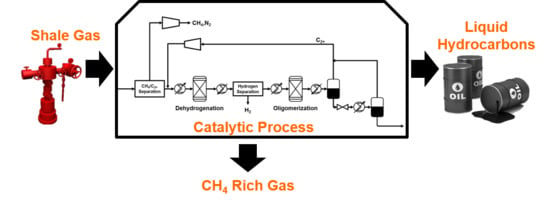
We propose a process that can upgrade shale condensate into liquid hydrocarbons via catalytic dehydrogenation followed by catalytic oligomerization. In this work, we only focus on converting ethane, propane, and butane in shale condensate into liquid fuel, and we do not consider the coupling of methane.
2. Thermodynamic Analysis of the NGL-to-Liquid Pathways
As mentioned earlier, apart from catalytic dehydrogenation followed by oligomerization, there are other routes to upgrade NGL to liquid fuel feedstocks. Alkenes or syngas are common intermediates for these routes. Taking ethane as an example, ethane can be converted to either ethylene or syngas and then upgraded to liquid fuel. Now for a comparison of different synthetic routes from NGL to liquid fuel, the energy demands of different pathways of ethane conversion are evaluated. For our current analysis, we only consider ethane to octane conversion.
Figure 2 below summarizes the different pathways for the thermodynamic analysis that will be discussed.
For the “ethane–ethylene–octane” route, we consider two different dehydrogenation methods: catalytic dehydrogenation and steam cracking. For catalytic dehydrogenation, the ethane is assumed to be converted to ethylene with 100% selectivity and the conversion of ethane is 45% according to reported experimental results; for steam cracking, the conversion of ethane is 67% and selectivity towards ethylene is 81% [
20,
28]. The catalytic dehydrogenation reactor and steam cracker are both operated at 900 K and 3.5 bar. The dehydrogenation unit is followed by the oligomerization reactor, in which ethylene is coupled to produce octane. The oligomerization reactors are operated at 600 K. Although the coupling reaction is exothermic, the generated heat cannot be recovered to provide heat for the dehydrogenation due to the lower oligomerization operating temperature. Therefore, to compare the energy consumption, we only consider the dehydrogenation units. Through Aspen Plus simulation, with pure ethane feed, the heat duties are 65 MJ/kmol of ethane reacted and 144 MJ/kmol of ethylene produced for the catalytic dehydrogenation reactor and 103 MJ/kmol of ethane reacted and 190 MJ/kmol of ethylene produced for the steam cracker, respectively. The actual ethane dehydrogenation reactions within the two dehydrogenation reactors are similar, and the difference in heat duty comes from the different conversion and the generation of byproducts in steam cracking. Furthermore, if we consider that the generation of high-temperature steam also demands energy input, catalytic dehydrogenation is a less-energy-intensive route for ethane conversion.
Another possible route from ethane to liquid fuel is via syngas. Ethane can be partially oxidized to syngas either by oxygen or steam and followed by a Fischer–Tropsch reactor for fuel synthesis. Considering the energy demand for air separation, we only consider ethane partial oxidation by steam. At 1000 K and 3.5 bar (the same condition as dehydrogenation), ethane and steam are reacted to produce syngas. The REQUIL reactor model in Aspen Plus was used to model the reformer or oxidation reactor. In this process, the reformer reactor consumes 349 MJ/kmol of ethane, which is higher than that of the dehydrogenation reactor. In addition, this process is counterproductive, as ethane is decomposed to carbon monoxide and hydrogen which are then later recombined to form long carbon chain molecules through Fischer–Tropsch or methanol-to-gasoline technology. Furthermore, in this process, high-temperature steam has to be generated, and the gas product from the oxidation reactor has to be compressed in order to go through the Fischer–Tropsch process. Once again, the large amount of heat generated in the Fischer–Tropsch process is at a much lower temperature than the reformer temperature, leading to a substantial degradation in the quality of heat. Therefore, among the three routes discussed, catalytic dehydrogenation followed by oligomerization is the most energy efficient method of light alkane upgrading.
3. Problem Statement
Given a shale gas condensate stream from a remote reservoir, it is desired to synthesize, simulate, and integrate an NGL-to-liquid hydrocarbons (NTL) process using catalytic dehydrogenation and oligomerization reactions and to carry out economic analysis to answer the following questions:
What is the necessary pretreatment of shale gas?
What is the correct flow sheet to achieve the NTL conversion?
What separation technologies are required for the process?
What are the economic criteria of the process and how do they compare with existing processes?
What is the cost differential between this process and existing GTL processes?
The following assumptions, basis, and data were used in all processes considered here:
The Bakken field is located in a remote part of North Dakota. Currently, the pipeline infrastructure is already at its full capacity, and the state’s natural gas consumption is well below its shale gas production [
29]. Considering the variability and decay of shale resource production, installing infrastructure for NGL distribution may not be attractive, as the payback period can easily exceed the well production lifetime [
3]. Therefore, it is desirable to convert the NGL locally into liquid fuel components, as it can be refined and marketed locally and nationally through various distribution channels. A 96 million standard cubic feet per day (MMSCFD) basis feed flow rate was selected because a typical single wellhead production rate in the Bakken field ranges from 1 to 4.8 MMSCFD, and this flow rate represents a medium-scale facility that processes outputs from between 20 and 100 wells [
3]. The composition of this stream is shown in
Table A3 in
Appendix D. Additional process assumptions shown in
Table 1 are also considered.
4. Process Description
Shale gas requires the same conventional gas treatment as natural gas. As gas treatment is a well-known technology and UOP-ThomasRussell has an operating modular field-erected gas treatment plant with a current proven size of 200 MMSCFD, we begin with conventional shale gas treatment which consists of acid gas and water removal [
15]. Depending on the nitrogen content of the raw shale gas, nitrogen removal may be necessary to meet the typical natural gas pipeline specifications, which is ≤4 mol % for nitrogen. In the case of the Bakken field, nitrogen removal may not be required because the region is known to produce both nitrogen-rich and nitrogen-deficient shale gas streams, and the two types of streams can be easily mixed in order to meet the pipeline specification.
Both acid gas and water removal processes are well-established and understood. Depending on the content of acid gas and water, there are various process options. Methyl diethyl amine (MDEA) absorption and triethylene glycol (TEG) absorption are the most common processes for acid gas and water removal, respectively. These processes are capable of reducing the acid gas content down to 4 ppm and the water content to 100 ppm [
30]. After the shale gas is treated, it is termed dry, sweet shale gas, which can then undergo further downstream processing.
Catalytic dehydrogenation is the next step and, in this unit operation, ethane, propane, and butane undergo dehydrogenation with a catalyst that reduces selectivities toward undesirable byproducts. The dehydrogenation of ethane is an endothermic reaction, and in order to achieve a reasonable equilibrium conversion, the reaction must be performed at moderately high temperature (900–1100 K).
Hydrogen generated during dehydrogenation may need to be removed prior to the oligomerization reaction, as it can re-saturate olefins. If the oligomerization catalyst has a high hydrogen tolerance such that selectivity toward hydrogenation products is low, then hydrogen can remain in the mixture. Otherwise, hydrogen must be removed, and this separation task can be accomplished using cryogenic distillation or gas membrane separation.
After selectively dehydrogenating ethane, propane, and butane at moderately high temperature, the resulting olefins can be converted to higher molecular weight hydrocarbons through an oligomerization reaction. Catalysts for oligomerization are available, and have been used for similar applications in the past [
26,
31]. The product of the oligomerization reaction is a mixture of high molecular weight hydrocarbons and unconverted light alkenes. Due to a large difference in their boiling points, high molecular weight hydrocarbons can be recovered through condensation by cooling the mixture. Then, the remaining vapor, which contains unconverted light alkenes, is recycled to the inlet of the catalytic dehydrogenation reactor.
5. Process Modeling
5.1. Gas Treatment
As stated earlier, acid gas treatment and water removal are well-known processes, and the selection of the specific process depends highly on the concentration of the acid gas and water in the shale gas stream. Based on the literature, MDEA sweetening and TEG dehydration processes are suitable for the Bakken field shale gas [
30]. In MDEA amine sweetening, MDEA solution is contacted with the shale gas, and carbon dioxide and hydrogen sulfide react with the amine solution. Then, the amine solution is regenerated in a stripper by releasing the acid gas from the solution. For water removal, TEG (triethylene glycol) solution is contacted with the sweet gas shale, where the water is ionically bonded with the TEG solution. The TEG solution is then recovered in a boiler by vaporizing the water. In this work, the economics and energy input of these processes are not considered as in other GTL processes. A treated natural gas stream is assumed as the feed.
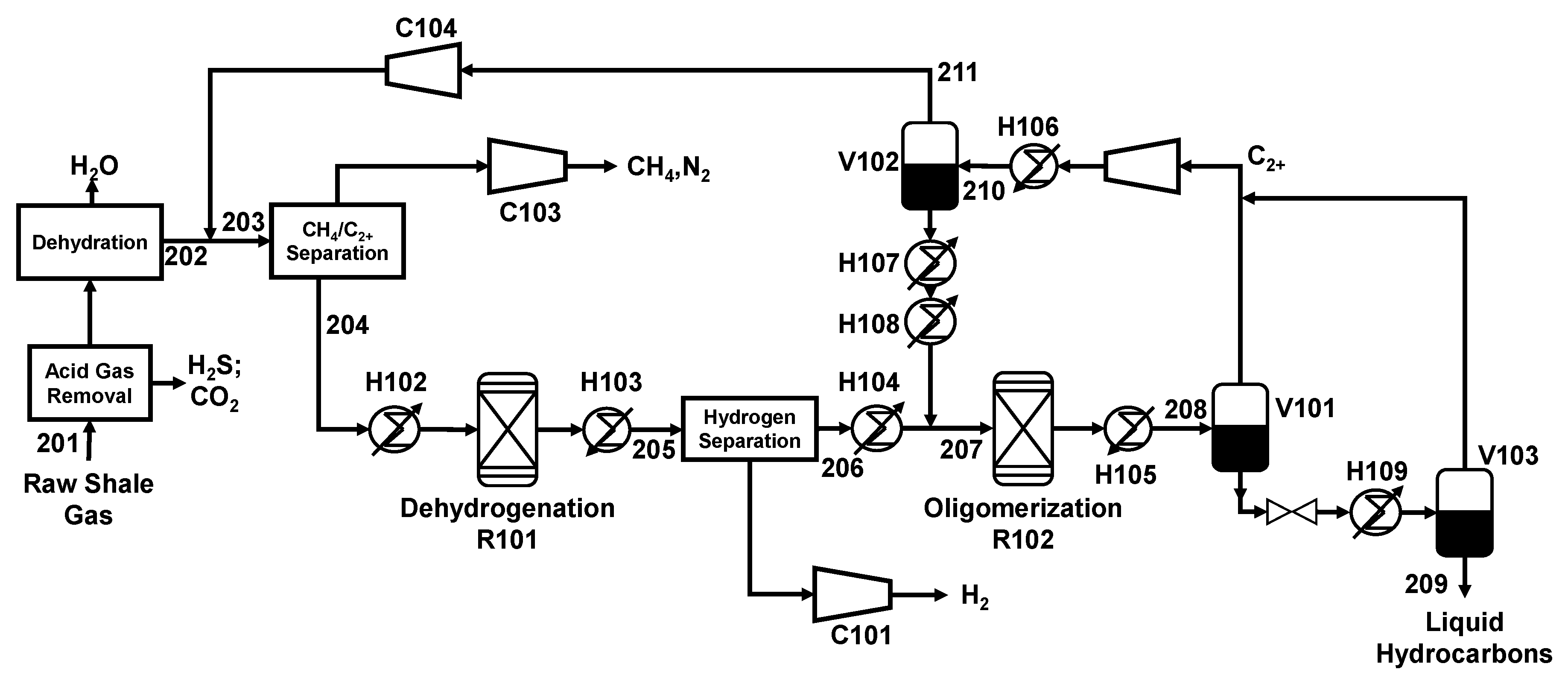
5.2. Demethanizer
After gas treatment, NGL must be separated from the shale gas stream (
Figure 3: 102;
Figure 4: 204). As methane is not converted to liquid hydrocarbons, a high concentration of residual methane in the NGL stream from the demethanizer can possibly lead to large accumulation in downstream recycle loop. Conventionally, cryogenic distillation is used for the demethanizer. Due to the potential of relatively small-scale application of this process, membrane separation is also considered for NGL separation, which has proven to be a viable and practical option in NGL recovery from natural gas [
32,
33]. Considering the limitations of existing CH
4-NGL separation processes, we propose two process designs based on methane recovery of 86% and 96% in the demethanizer section, and they are labeled Process I and Process II, shown in
Figure 3 and
Figure 4. For the 96% recovery demethanizer, a turbo-expander process scheme with a distillation column modeled using RadFrac in Aspen Plus was used [
34]. For 85% recovery, cascade gas membrane separation was used, and cost calculation for this unit operation was based on a well-mixed membrane model. Note that the turbo-expander process scheme can also be employed for the 85% recovery, and the cascade membrane here was selected to illustrate the deployment of other separation technologies apart from distillation. The detailed schemes for these unit operations can be found in the Supplementary Information. The membrane was assumed to have a permeability of 120 barrer for C
2+ and permselectivity of 12 for CH
4/CH
2+ [
35]. The capital cost of the membrane module was assumed to be
$50/m
2.
5.3. Dehydrogenation
Ethane, propane, and butane can be transformed to its corresponding mono-olefins through catalytic dehydrogenation. The dehydrogenation reaction can be generalized as follows:
The reaction is endothermic, and for light hydrocarbons, the equilibrium conversion is reasonable at high temperature ranging between 800 K and 1100 K [
36]. Based on Le Chatelier’s principle, lower pressure shifts the chemical equilibrium toward the product side. Hence, the reaction should be operated at low pressure. Currently, the industrial catalytic dehydrogenation of light hydrocarbons is limited to only propane and butane. Honeywell Oleflex is an example of the industrial implementation of catalytic dehydrogenation which entails the dehydrogenation of propane to propylene [
26]. Using PtSn/Al
2O
3 catalyst, propane is dehydrogenated at 1.4 barg and 873 K. The dehydrogenation of ethane is usually achieved through steam cracking [
26]. Ethane conversion of 45% with selectivity of 99% toward ethylene has been reported at 873 K using PtZn/SiO
2 catalyst [
20].
Here, we assumed that through catalyst development, 95% of equilibrium conversion of ethane, propane, and butane dehydrogenation at 1073 K and 6.58 bar can be reached. Note that for dehydrogenation, 95% of the true equilibrium conversion was considered in order to account for the fact that dehydrogenation is a highly endothermic reaction and heat transfer is the rate-limiting step. In
Figure 3, R101 represents the catalytic dehydrogenation reactor and 103 is the inlet stream to R101. The REQUIL reactor model in Aspen Plus was used. Three reactions (dehydrogenation of ethane, propane, and butane), and their respective temperature approaches were specified in order to adjust the equilibrium conversion. No competing reactions (e.g., hydrogenolysis of alkanes) were considered. The same modeling details for the dehydrogenation reactor were applied for Process II in
Figure 4.
5.4. Hydrogen Recovery
The product stream (
Figure 3, 104;
Figure 4, 205) from the dehydrogenation reactor which contains mono-olefins, hydrogen, and unconverted light alkanes is then cooled down to 500 K. Using membrane separation, hydrogen will be partially recovered. Some retained hydrogen in the retenate stream is desirable to ensure the stability of the dehydrogenation and oligomerization catalyst [
20]. In Aspen Plus, the membrane was simulated using a separator and calculator block. Within the calculator block, the material balance and design equation for a well-mixed membrane were employed and the output from this block was used in the separator block to determine the purity and flow rate of the permeate and retenate streams. For sizing and economics calculation, a well-mixed membrane system and
$50/m
2 capital cost for a spiral wound membrane module were assumed [
37]. The hydrogen membrane used in this work was assumed to have permeability of 250 barrer for hydrogen and selectivity of 590 and 125 for hydrogen/ethylene and hydrogen/methane, respectively [
33,
38]. The gas membrane was modeled as a well-mixed membrane system with a binary feed, and a polyimide membrane was used. In addition, it was assumed that the feed was a binary mixture of hydrogen and pseudo component of C
1+. The permselectivity of H
2/C
1+ for this membrane here was taken to be 483. The gas membrane was designed to achieve a target of 15% mole of hydrogen in the retenate stream in order to stabilize the catalysts used in this process. The permeate purity was 83.87% mole of hydrogen. The net recovery of hydrogen through the membrane was 0.105 kmol of H
2/m
2 h. Using a single membrane configuration and setting the pressure of the permeate side at 1 bar, the hydrogen removal in the permeate was 54% and ethane slip to the permeate stream was 16%. This resulted in 15% mole of hydrogen in the retenate stream according to our simulation results.
5.5. Oligomerization
The retentate stream (
Figure 3, 105) from the hydrogen membrane unit was heated to 573 K and then fed to the oligomerization reactor. In this reactor, olefins couple together to form higher molecular weight olefins. For the oligomerization of olefins , the reaction can be generalized as follows:
The oligomerization reaction is exothermic and generally runs at low temperature [
26]. This reaction is carried out at 573 K and 5.47 bar [
26] H-ZSM-5 is commonly used for the olefin oligomerization reaction [
31]. It has been reported that 90 wt % conversion to liquid has been observed from propene at 500 K and 24 bar with 88% of the liquid being C
9+ hydrocarbons [
39]. Similarly, ethylene fed with nitrogen at 773 K obtained a yield of 54.2% toward C
5+ hydrocarbons on H-ZSM-5 [
40]. Toch et al. also reported 99% ethylene conversion with 25% and 55% selectivities toward propene and gasoline, which is hydrocarbon with a carbon number ranging from five to eight, using Ni-beta zeolite at 500 K and 1.0 MPa [
41,
42].
In this work, we assumed that this chemical system achieves thermodynamic equilibrium at 600 K and 5.47 bar and only alkene coupling that produces a larger alkene occurs. Therefore, we only considered the C
4–C
12 alkene oligomerization products. The selectivity to various high molecular weight alkenes are defined based on equilibrium. In
Figure 3, R102 represents the oligomerization reactor. The RGIBBS reactor model in Aspen Plus was used to estimate the equilibrium composition. In addition, all paraffin molecules, methane, and hydrogen were set to be inert, indicating that they do not participate in the minimization of Gibbs free energy calculation. Note that in these coupling reactions, it is very likely for the olefins to also form both cyclic and branched molecules, but this was not considered in this study.
5.6. Liquid Hydrocarbon Recovery
After the oligomerization reactor, the final step is to recover liquid hydrocarbons and recycle the unconverted C
2 and C
3 into either of the reactors depending on whether they are olefinic or aliphatic light hydrocarbons. First, the product stream (
Figure 3, 106) from the oligomerization reactor is cooled down to 275 K to condense liquid hydrocarbons. This temperature was selected because C
9+ hydrocarbons may form into waxes and solids below 275 K. The downstream processing of the vapor stream is a crucial step in the overall separation process. This vapor stream mainly contains unconverted olefinic and aliphatic light hydrocarbons. If this vapor stream is directly recycled to the fresh feed stream of the dehydrogenation reactor and the methane recovery in the upstream CH
4/C
2+ separator is not very high, this necessitates a very large recycle ratio. With a large recycle ratio, the feed stream entering the dehydrogenation reactor may be compositionally worse than the shale gas composition. There are several separation and recycle process configuration options to avoid a large recycle ratio, and here we consider the two following configurations:
In the first configuration, labeled Process I, the vapor stream coming out of the condenser (
Figure 3, V101) after the oligomerization reactor is directly recycled to the fresh NGL stream entering the dehydrogenation reactor R101 (Process I,
Figure 3). In order to avoid a large accumulation of methane, the CH
4/C
2+ separation step must recover a large percentage of methane. For 86% and 96% methane recovery, the recycle ratios are 4.8 and 1.4, respectively, for Process I. Membrane separation can achieve 86% recovery, but it is difficult to achieve 96% recovery, which may require refrigeration and/or a multiple-stage cascade membrane system [
37,
43]. Thus, for Process I, the CH
4/C
2+ separation step was designed to recover 96% of the methane in the feed.
The second configuration, labeled Process II, entails multiple recycle loops (Process II,
Figure 4). By compressing and cooling the vapor stream (
Figure 4, 210) to 275 K, a liquid stream containing up to 30% mono olefins of C
2, C
3, and C
4 and 40% of C
2, C
3, and C
4 alkanes is obtained, and combining this liquid stream with the feed to the oligomerization reaction results in the two recycle loops shown in
Figure 4. This results in smaller recycle ratios compared to those of Process I, as the light alkenes are reacted in the oligomerization reactor. The vapor stream (
Figure 4, 211) from the second condenser (
Figure 4, 211) contains up to 20% methane. After compressing the vapor to 30 bar, the vapor is combined with the incoming shale gas stream (
Figure 4, 202). This setup results in two loops. Each loop has a recycle ratio of less than two.
We proposed and simulated two different process designs for NGL-to-liquid fuel using Aspen Plus. The stream-data results of processes I and II are shown in
Table 2 and
Table 3, respectively. These data were used to perform the techno-economic analysis.
6. Results and Discussion
As mentioned earlier, REQUIL and RGIBBS reactor models were used to model catalytic dehydrogenation and oligomerization reactions, respectively. For dehydrogenation, the conversions of ethane, propane, and butane per pass were 37.76%, 65.63%, and 50.16%, respectively, for Process I and Process II. In steam cracking, the molar conversion of ethane to ethylene is approximately 70% and the main by-product is a hydrogen-rich off gas [
28]. Clearly, the catalytic molar conversion of ethane to ethylene is lower, but reported catalyst for the dehydrogenation of ethylene has shown to have high selectivity toward the dehydrogenation of ethane and to suppress the hydrogenolysis of ethane to methane. One of the performance metrics is the overall amount of C
2+ being converted to C
4+. Equation (
3) defines this metric as follows:
where
is the molar flow rate of hydrocarbons with carbon number
i in the dry and sweet shale gas stream and
is the molar flow rate of the hydrocarbons with carbon number
i in the final liquid hydrocarbon, hydrogen-rich, and methane-rich streams (
Figure 3: liquid hydrocarbons; H
2; CH
4, N
2). The overall C
2+ conversion was calculated to be 76% and 72% for Processes I and II, respectively. The loss of reactants is due to the purge streams and gas membrane separation. These conversions translate to 139 and 141 BPD of liquid hydrocarbons per MMSCFD of shale gas from the Bakken field used in our simulation. Existing GTL plants using natural gas yield approximately 134 BPD per MMSCFD [
44]. Both Processes I and II achieve similar yields. It is estimated that the hydrocarbon yield from syngas followed by Fischer–Tropsch is 135 bbl/MMSCF of ethane, and gasoline yield from syngas followed by methanol synthesis and methanol-to-gasoline is 111 bbl/MMSCF of ethane. The main distinctions between the two proposed processes are the process complexity, the degree of methane recovery, and their economics. Process I only possesses one recycle loop and fewer unit operations compared to Process II, which has two recycle loops and more unit operations. Demethanization in Process I cannot be achieved using existing membrane technology, while in Process II, gas membrane separation is viable for methane removal.
6.1. Energy Integration
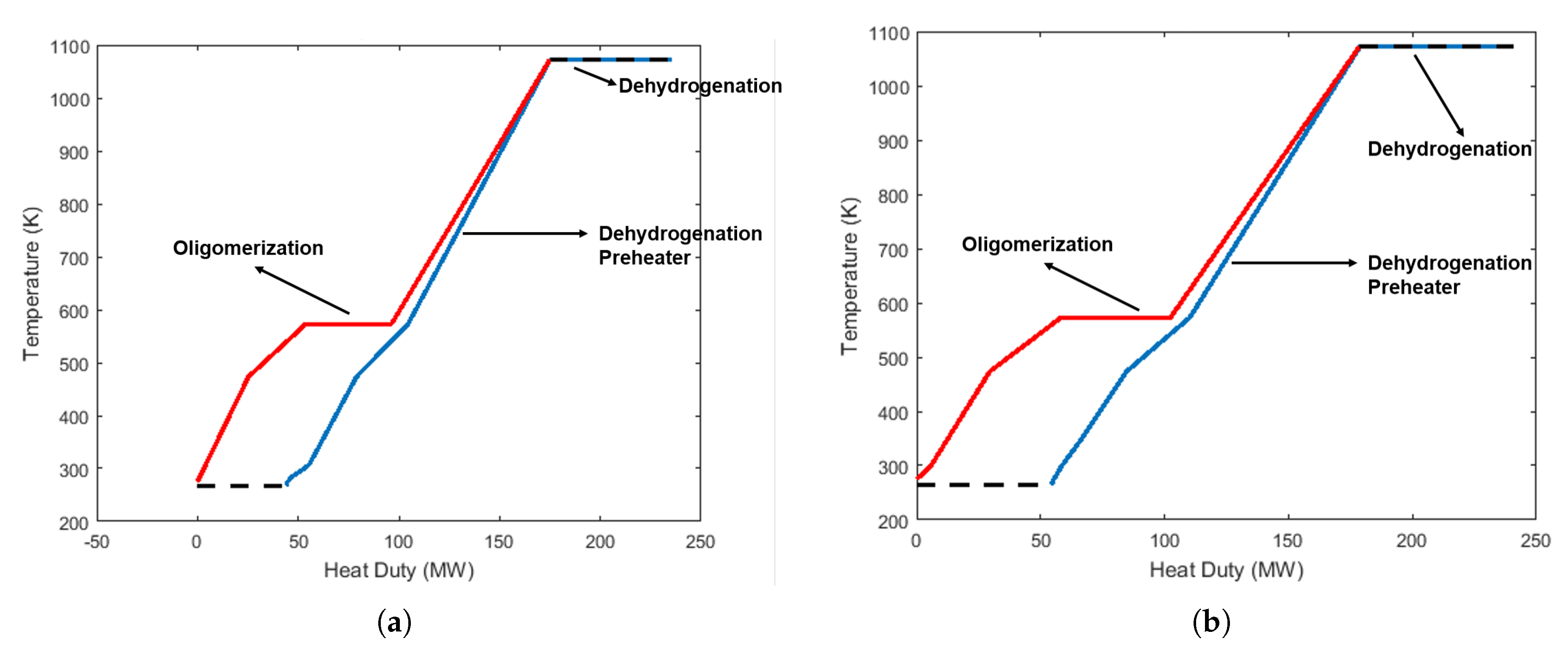
Each process design has several process cooling and heating duties. Within the recycle loop, the recycle stream is heated to 1073 K from ambient temperature (308 K) after being combined with the fresh feed stream. The final liquid hydrocarbon stream is brought back to ambient temperature and pressure. Additionally, the dehydrogenation and olefin coupling reactions are endothermic and exothermic, respectively. Operating costs include cooling and heating duties. Integrating these duties can reduce the overall operating cost, since identifying one heat integration results in two operating cost savings, heating and cooling duties. Thermal pinch analysis can be used to determine the best heat integration in a process. The Aspen Energy Analyzer was used to determine the minimum heating and cooling duties for the two process designs considered here.
As shown in
Figure 5a,b, the minimum heat duty is the horizontal gap between the cooling (blue line) and the heating curve (red line). For Process I, it was 64 MW, which is the heat of reaction for dehydrogenation. Thermal pinch results also indicated that the heat duty requirement could be reduced by 72%. For Process II, it was 65 MW, which is approximately the heat of reaction for dehydrogenation. Both minimum heat duties are equivalent to the heat of the reaction in dehydrogenation. Hence, the heat flows within the loops were being integrated except for the dehydrogenation, as it demands heat at 1073 K and no other unit operation generates heat at that temperature. The minimum cooling duty can further reduce the electricity consumption through the means of co-generation [
45,
46].
Using the heating and cooling utilities prior to heat integration, the process thermal efficiency was calculated and shown in
Table 4. For the efficiency calculation, the energy inputs were set on the basis of primary energy and the products were taken to be only liquid hydrocarbons. Hydrogen and pipeline quality gas were considered. The equation below describes this efficiency:
where
is the mass flow rate of stream
i,
is the lower heating value of stream
i,
is the total heat consumption from heat exchangers and reactors, and
is the total heat consumption for electricity. These efficiencies are higher compared to GTL-FT (Fischer–Tropsch) and GTL-MTG (methanol-to-gasoline) efficiencies of 56% and 41%, respectively. Of course, GTL-FT releases a large amount of heat from the Fischer–Tropsch reactor that could be used for co-generation to improve that process efficiency. The catalytic dehydrogenation of light alkanes followed by oligomerization has the potential to be more efficient than existing technologies.
6.2. Economics
In order to measure the economic performance of the processes proposed in this study, an economic analysis was performed to estimate the total capital investment (TCI) and return-on-investment (ROI). Standard procedures were used to assess those economic parameters [
45].
Table 5 summarizes the cost parameters that were assumed and the operating costs of both processes. Note that here we are only considering the NGL from shale gas and the resulting liquid hydrocarbon product. Hence, we are not considering the capital cost for methane gas treatment and revenue gained from methane. As shown in
Table 5, the main difference between the operating costs of Process I and Process II lies in the electricity consumption.
6.2.1. Total Capital Investment (TCI)
In order to estimate the total capital investment, two techniques were used together to estimate the capital cost of each unit operation. First, standard sizing algorithms and calculation in Aspen Economic Analyzer were used to estimate most of the unit operations. Second, a combination of cost charts, Lang’s method, and estimates from various pieces of literature were used to estimate the dehydrogenation reactor and other unit operations [
45,
47].
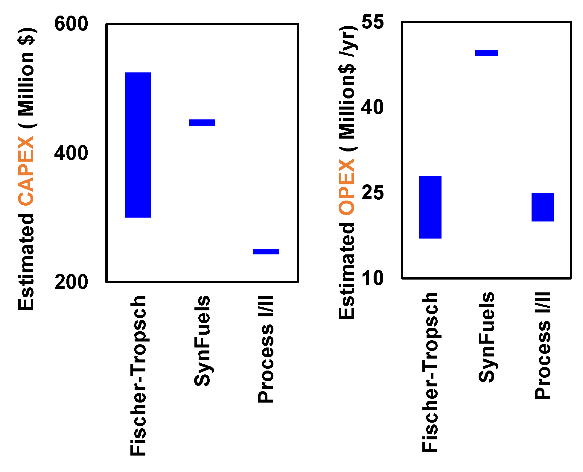
Table A1 and
Table A2 in the Supplementary Information summarize the TCI distribution for these processes and also the technique used for each unit operation. The estimated TCIs for Process I and Process II were
$251 million and
$243 million, respectively. For comparison with other existing processes (i.e., GTL-FT and GTL-MTG), to produce the same amount of liquid hydrocarbons, GTL–FT costs between 300 to 525 million USD [
17,
18] and GTL–MTG costs approximately 1.5 billion USD [
28,
48]. SynFuels International Inc.’s GTL process is estimated to have TCI of
$135 MMUSD for 20 MMSCFD. Using the sixth-tenth rule, the estimated capital cost for a 90 MMSCFD plant is
$332 MMUSD.
Figure 6 highlights the comparison of the processes in this work with other existing technologies. The TCI for the processes proposed here was at least 17% less than the alternate technologies.
6.2.2. ROI and Payback Period
Besides the TCI, ROI is generally used to determine the economic feasibility of a plant. In order to calculate these values, the following assumptions are made: (1) linear depreciation model of five year period with 10% salvage value at the end of the period; (2) tax rate is 30% and the discount rate is 10%. Further details on the ROI evaluation can be found in
Appendix B. The ROI is calculated to be 0.52 and 0.54 for Processes I and II, respectively. A process with an ROI of 0.15 or higher is considered to be lucrative. The slight difference in ROI of Processes I and II is due to the difference in the TCI of the two processes. Although Process II has a higher operating cost and a lower C2 and C3 recovery. The annual net income for this process is higher because of the lower depreciation. Therefore, this results a slightly higher ROI compared to Process I. Despite Process II having a slightly higher ROI, Process I involves a demethanizer with 95% methane recovery, which can be difficult to achieve using membrane separation technology. Note that a gas membrane system is generally deployed for gas plants of size less than 100 MMSCFD and the size of the plant considered here is 96 MMSCFD. Therefore, the ROI difference between these two processes may widen at smaller plant sizes.
The ROI values can be directly translated into payback period. The payback periods for Processes I and II are 1.9 years and 1.8 years, respectively. Considering the decline of well productivity, which can be up to 75% within three years, the payback periods of these processes are well within the lifetime of these wells [
49].
7. Potential of the Proposed Processes for Modularization
Considering the economic opportunity presented by either stranded shale gas or associated shale gas, the proposed process can be deployed at modular scales. In a modular plant, the process equipment and its supporting components are mounted within a structural metal framework and each module is a self-contained process [
50]. There are many factors that determine whether a process is amenable to modularization, and process complexity is one of the main factors. As stated previously, many of the existing technologies for thes conversion of natural gas liquid to liquid fuel have only been implemented at large scale. Steam cracking plants generally process up to 1500 MM lbs/year. The smallest proved GTL plant using Fischer–Tropsch process that has been proven is 14,700 bbl/day. These GTL processes mainly consist of syngas generation followed by Fischer–Tropsch or methanol synthesis with methanol-to-gasoline (MTG).
Each process described in this study is amenable to process modularization. However, the proposed process has been shown to be potentially more economically lucrative assuming high selectivity of catalytic dehydrogenation and considering the large boiling point difference between liquid hydrocarbons and light hydrocarbons. Steam cracking requires either downstream upgrading and/or separation in order to hydrogenate acetylene or remove methane. Fischer–Tropsch synthesis produces a liquid product that requires hydrogenation and hydrocracking. Therefore, the existing NTL processes clearly require more unit operations than the proposed NTL process. Although the economics of modular NTL proposed in this work have not been evaluated, this NTL process has the potential to be more economically modularized compared to other existing technologies.
8. Conclusions
Shale gas is projected to be one of the dominant forces in the future of the United States energy landscape. With a projected supply for more than one hundred years, fitting the shale gas into the United States energy landscape requires processes that can convert shale gas into different forms of energy. Shale gas utilization can vary widely from electricity production to chemical production. However, existing infrastructure and market saturation do not allow for some of its common utilizations, particularly as chemical feedstock for olefin plants. However, converting shale gas to liquid fuel can overcome limitations from existing infrastructure, as liquid fuel is transportable and easily marketed. Several large shale gas fields are located in historically non-gas-producing regions (e.g., Bakken and Niobrara basins), where infrastructure for gas distribution is limited or non-existent. Liquid hydrocarbons can be easily transported through different channels such as railways and trucks for further refining. In addition to this, the liquid fuel market is widely distributed with minimal time-variant demand. Herein, we proposed a process for the transformation of shale gas that converts the NGL in shale gas into liquids using a catalytic system that differs from the existing technologies.
There were two processes proposed in this study depending on the separation technology that is considered. Both processes entail dehydrogenation and oligomerization reactions. The main distinctions between the two processes are the separation technology used for the demethanizer and the recycle loop configurations. In terms of energy consumption, both processes have similar minimum heating and cooling duties and product yield. The main difference in energy consumption between these two processes is the electricity consumption. Based on the evaluated economic indicators, Process II is more economically attractive than Process I. In addition, it is not clear whether the demethanizer separation target in Process I can be achieved using membrane technology solely and whether Process I is amenable to modularization for wellhead applications.
Existing GTL-FT and GTL-MTG processes are estimated to be economically less attractive than the proposed processes. The total capital costs of Processes I and II are estimated to be at least 17% lower than that of the conventional GTL processes. The payback periods of Processes I and II are about two years. Clearly, the proposed processes are expected to be much more lucrative than existing technologies.
This study only considered regional or gathering scale facilities. Varying the scale of this proposed process can impact not only its economics, but also the economics and supply chain of NGL, liquid fuels, and other end-use products, especially when the entire chemical manufacturing industry is considered. It is worth assessing how this process fits into the current United States chemical manufacturing industry.
Author Contributions
Conceptualization, E.G., J.J.S., J.T.M., F.H.R. and R.A.; Formal Analysis, T.R., Y.L. and J.J.S.; Funding Acquisition, J.T.M, F.H.R., and R.A.; Investigation, T.R. and R.A.; Methodology, J.T.M, J.J.S, and R.A.; Project Administration, F.H.R. and R.A.; Writing—Original Draft, T.R.; Writing—Review & Editing, Y.L., E.G., J.J.S. and R.A.
Funding
This paper is based upon work funded in part by the National Science Foundation under Cooperative Agreement No. EEC-1647722. Any opinions, findings and conclusions or recommendations expressed in this material are those of the author(s) and do not necessarily reflect the views of the National Science Foundation.
Acknowledgments
We would like to acknowledge CISTAR (Center for Innovative and Strategic Transformation of Alkane Resources) for partial funding. In addition, we would like to acknowledge helpful and insightful discussion with David T. Allen from the McKetta Department of Chemical Engineering, University of Texas—Austin.
Conflicts of Interest
The authors declare no conflict of interest. The founding sponsors had no role in the design of the study; in the collection, analyses, or interpretation of data; in the writing of the manuscript, and in the decision to publish the results.
Abbreviations
The following abbreviations are used in this manuscript:
| NGL | Natural Gas Liquids |
| HGL | Hydrocarbon Gas Liquids |
| MMSCFD | Million Standard Cubic Feet Per Day |
| EIA | Energy Information Agency |
| GTL | Gas-to-Liquids |
| NTL | NGL-to-Liquids |
| FT | Fischer–Tropsch |
| MTG | Methanol-to-Gasoline |
| TCI | Total Capital Investment |
| ROI | Return on Investment |
Appendix A. Economic Analysis
In this work, an economic analysis was performed to evaluate the total capital investment, operating cost, return-on-investment, and break even price for crude oil. For the total capital cost investment, a combination of standard procedure from Aspen Economic Analyzer and estimates from literature along with Lang’s method was used to obtain the total capital cost for each unit operation.
Table A1 and
Table A2 summarize the capital or the installed cost for each unit operation and their methodology. The summation of all unit operation costs listed in the tables below alone does not give the total capital cost. The Aspen Plus Economic Analyzer only provides the installed cost for each unit operation, and the values obtained using Aspen Plus Economic Analyzer in the tables below are the installed costs.
Table A1.
Equipment cost for unit operations in Process I.
Table A1.
Equipment cost for unit operations in Process I.
| Unit Operation | MMUSD | Method |
|---|
| Demethanizer Distillation Column System | 1.9 | Aspen Economic Analyzer |
| Hydrogen Membrane | 1.8 | Well-mixed membrane system and $50/m2 |
| HEX-101 | 0.018 | Aspen Economic Analyzer |
| HEX-102 | 4.8 | Aspen Economic Analyzer |
| HEX-103 | 1.37 | Aspen Economic Analyzer |
| HEX-104 | 0.43 | Aspen Economic Analyzer |
| HEX-105 | 0.14 | Aspen Economic Analyzer |
| Dehydrogenation Reactor | 4.6 | Aspen Economic Analyzer |
| Oligomerization Reactor | 1.8 | Aspen Economic Analyzer |
| COMP-102 | 5.2 | Aspen Economic Analyzer |
| COMP-103 | 0.99 | Aspen Economic Analyzer |
| COMP-104 | 11.2 | Aspen Economic Analyzer |
| V-101 | 0.18 | Aspen Economic Analyzer |
| V-102 | 0.16 | Aspen Economic Analyzer |
| Refrigeration | 14 | Aspen Economic Analyzer |
Table A2.
Equipment cost for unit operations in Process II.
Table A2.
Equipment cost for unit operations in Process II.
| Unit Operation | MMUSD | Method |
|---|
| Demethanizer Membrane System | 7.3 | Well-mixed membrane system and $50/m2 |
| Hydrogen Membrane | 1.0 | Well-mixed membrane system and $50/m2 |
| HEX-102 | 4.6 | Aspen Economic Analyzer |
| HEX-103 | 1.3 | Aspen Economic Analyzer |
| HEX-104 | 0.42 | Aspen Economic Analyzer |
| HEX-105 | 0.11 | Aspen Economic Analyzer |
| HEX-106 | 0.03 | Aspen Economic Analyzer |
| HEX-107 | 0.02 | Aspen Economic Analyzer |
| HEX-108 | 0.05 | Aspen Economic Analyzer |
| HEX-109 | 0.02 | Aspen Economic Analyzer |
| Dehydrogenation Reactor | 4.7 | Six Tenth Rule |
| Oligomerization Reactor | 1.8 | Aspen Economic Analyzer |
| COMP-101 | 11.2 | Aspen Economic Analyzer |
| COMP-102 | 5.2 | Aspen Economic Analyzer |
| COMP-103 | 0.74 | Aspen Economic Analyzer |
| COMP-104 | 1.73 | Aspen Economic Analyzer |
| Refrigeration | 14 | Aspen Economic Analyzer |
| V-101 | 0.18 | Aspen Economic Analyzer |
| V-102 | 0.16 | Aspen Economic Analyzer |
| V-103 | 0.16 | Aspen Economic Analyzer |
For the standard procedure from the Aspen Economic Analyzer, details can be found in the manual. Several of the unit operations (e.g., the dehydrogenation reactor, oligomerization reactor, and membranes) were estimated using literature values along with Lang’s method.
Appendix B. Economic Parameters Calculation
Appendix B.1. Return-on-Investment
The equation for ROI is the following:
The total capital investment is the sum of all unit operations’ total capital costs. The total capital investment can be calculated by summing values in
Table A1 and
Table A2, respectively, and multiplying this sum by Lang’s factor. The second value needed to calculate the ROI is the annual net (after tax profit) cash flow. To calculate the annual net (after tax profit) cash flow, the following equation was used:
where
is the total annual revenue,
is the annual operating cost,
is the annual feedstock cost, and
is the depreciation. Note that the assumed selling prices for all outlet streams and feedstock costs for all raw materials are listed in
Table 5. A linear depreciation model with a recovery period of five years was used to calculate the depreciation, which is given by the following:
Here, the recovery period was assumed to be five years and the salvage value was 10% of the TCI. The payback period can be calculated by taking the inverse of the return on investment.
Appendix C. CH4-N2/C2+ Separation
Appendix C.1. Demethanizer
In this process configuration, a turboexpander and a Joule–Thompson valve are used to provide the refrigeration needed to liquefy the natural gas stream.
Figure A1 below describes the industry standard turboexpander process employed in Process I.
Figure A1.
Turboexpander demethanizer scheme.
Figure A1.
Turboexpander demethanizer scheme.
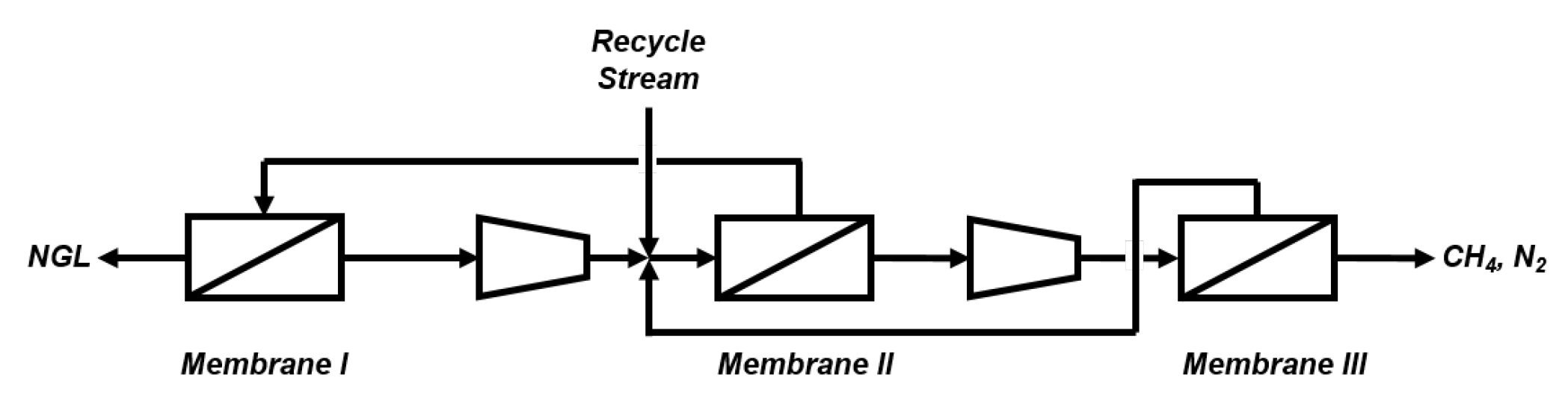
Appendix C.2. Cascade Gas Membrane Scheme
In this cascade gas membrane configuration, the pressure on the permeate side is atmospheric pressure and it is assumed that the pressure drop between the feed and retenate streams is negligible. The outlet pressure from every compressor is 10 bar. In order to achieve the desired 85% methane recovery, stage cuts for membranes I, II, and II were set as 1.3%, 53.4%, and 74.8%, respectively. In addition, the mole fractions of the most permeable component (in this case methane) in the retenate for membranes I, II, and III were 0.15, 0.15, and 0.39, respectively.
Figure A2 describes the cascade gas membrane configuration that is employed in Process II.
Figure A2.
Cascade gas membrane demethanizer scheme.
Figure A2.
Cascade gas membrane demethanizer scheme.
Appendix D. Shale Gas Composition
Table A3.
Composition of shale gas from the Bakken field in the United States [
2].
Table A3.
Composition of shale gas from the Bakken field in the United States [
2].
| Component | Mole Percentage-Bakken |
|---|
| CO2 | 0.57 |
| H2S | 0.29 |
| H2O | 0.15 |
| N2 | 5.20 |
| CH4 | 57.55 |
| C2H6 | 19.89 |
| C3H8 | 11.30 |
| n-C4H10 | 2.82 |
| i-C4H10 | 0.96 |
| n-C5H12 | 0.55 |
| i-C5H12 | 0.38 |
| C6H14 | 0.22 |
| C7H16 | 0.09 |
| C8H18 | 0.04 |
References
- Ehlinger, V.M.; Gabriel, K.J.; Noureldin, M.M.B.; El-Halwagi, M.M. Process Design and Integration of Shale Gas to Methanol. ACS Sustain. Chem. Eng. 2014, 2, 30–37. [Google Scholar] [CrossRef]
- He, C.; You, F. Shale Gas Processing Integrated with Ethylene Production: Novel Process Designs, Exergy Analysis, and Techno-Economic Analysis. Ind. Eng. Chem. Res. 2014, 53, 11442–11459. [Google Scholar] [CrossRef]
- Ka, B.; Pe, K. Compositional variety complicates processing plans for US shale gas. Oil Gas J. 2009, 107, 50–55. [Google Scholar]
- EIA. Natural Gas Pipeline Network—Transporting Natural Gas in the United States; EIA: Washington, DC, USA, 2008. [Google Scholar]
- DeRosa, S.E. Impact of Natural Gas and Natural Gas Liquids on Chemical Manufacturing in the United States. Ph.D. Thesis, University of Texas at Austin, Austin, TX, USA, 2016. [Google Scholar]
- Hydrocarbon Gas Liquids (HGL). Recent Market Trends and Issues; Technical Report; U.S. Energy Information Administration: Washington, DC, USA, 2014. [Google Scholar]
- Energy Information Administration. Short-Term Outlook for Hydrocarbon Gas Liquids; Technical Report; U.S. Energy Information Administration: Washington, DC, USA, 2016. [Google Scholar]
- He, C.; Pan, M.; Zhang, B.; Chen, Q.; You, F.; Ren, J. Monetizing shale gas to polymers under mixed uncertainty: Stochastic modeling and likelihood analysis. AIChE J. 2018, 64, 2017–2036. [Google Scholar] [CrossRef]
- Gong, J.; You, F. A new superstructure optimization paradigm for process synthesis with product distribution optimization: Application to an integrated shale gas processing and chemical manufacturing process. AIChE J. 2018, 64, 123–143. [Google Scholar] [CrossRef]
- Growing U.S. HGL Production Spurs Petrochemical Industry Investment—Today in Energy; U.S. Energy Information Administration (EIA): Washington, DC, USA, 2015.
- Goellner, J.F.; Hamilton, B.A. Expanding the Shale Gas Infrastructure. Chem. Eng. Progress 2012, 49–59. [Google Scholar]
- Mallapragada, D.S.; Duan, G.; Agrawal, R. From shale gas to renewable energy based transportation solutions. Energy Policy 2014, 67, 499–507. [Google Scholar] [CrossRef]
- Mallapragada, D.S.; AgrawAL, R. Role of Natural Gas in America’s Energy Future: Focus on Transportation; Purdue Policy Research Institute (PPRI): West Lafayette, IN, USA, 2013; p. 6. [Google Scholar]
- The Outlook for Energy: A View to 2040; Technical Report; ExxonMobil: Irving, TX, USA, 2016.
- Russell, T.H. Changes of Cryogenic, Amine Plant and Standard Plant Concept; Thomas Russell Co.: Tulsa, OK, USA, 2011; pp. 1–18. [Google Scholar]
- Cantrell, J.; Bullin, J.A.; McIntyre, G.; Butts, C.; Cheatham, B. Economic Alternative for Remote and Stranded Natural Gas and Ethane in the US; Bryan Research and Engineering, Inc.: Bryan, TX, USA, 2016. [Google Scholar]
- Lutz, B. New Age Gas-to-Liquid Processing. Hydrocarb. Eng. 2001, 6, 23–28. [Google Scholar]
- Senden, M.; McEwan, M. The Shell Middle Distillates Synthesis (SMDS) Experience. In Proceedings of the 16th World Petroleum Congress, Calgary, AB, USA, 11–15 June 2000. [Google Scholar]
- Wu, Z.; Wegener, E.C.; Tseng, H.T.; Gallagher, J.R.; Harris, J.W.; Diaz, R.E.; Ren, Y.; Ribeiro, F.H.; Miller, J.T. PdIn intermetallic alloy nanoparticles: Highly selective ethane dehydrogenation catalysts. Catal. Sci. Technol. 2016, 6, 6965–6976. [Google Scholar] [CrossRef]
- Cybulskis, V.J.; Bukowski, B.C.; Tseng, H.T.; Gallagher, J.R.; Wu, Z.; Wegener, E.; Kropf, A.J.; Ravel, B.; Ribeiro, F.H.; Greeley, J.; et al. Zinc Promotion of Platinum for Catalytic Light Alkane Dehydrogenation: Insights into Geometric and Electronic Effects. ACS Catal. 2017, 7, 4173–4181. [Google Scholar] [CrossRef]
- Sattler, J.J.H.B.; Ruiz-Martinez, J.; Santillan-Jimenez, E.; Weckhuysen, B.M. Catalytic Dehydrogenation of Light Alkanes on Metals and Metal Oxides. Chem. Rev. 2014, 114, 10613–10653. [Google Scholar] [CrossRef] [PubMed]
- Baroi, C.; Gaffney, A.M.; Fushimi, R. Process economics and safety considerations for the oxidative dehydrogenation of ethane using the M1 catalyst. Catal. Today 2017, 298, 138–144. [Google Scholar] [CrossRef]
- Chen, K.; Bell, A.T.; Iglesia, E. Kinetics and Mechanism of Oxidative Dehydrogenation of Propane on Vanadium, Molybdenum, and Tungsten Oxides. J. Phys. Chem. B 2000, 104, 1292–1299. [Google Scholar] [CrossRef] [Green Version]
- Wolf, D.; Dropka, N.; Smejkal, Q.; Buyevskaya, O. Oxidative dehydrogenation of propane for propylene production—Comparison of catalytic processes. Chem. Eng. Sci. 2001, 56, 713–719. [Google Scholar] [CrossRef]
- Ren, T.; Patel, M.; Blok, K. Olefins from conventional and heavy feedstocks: Energy use in steam cracking and alternative processes. Energy 2006, 31, 425–451. [Google Scholar] [CrossRef] [Green Version]
- Meyers, R.A. Handbook of Petroleum Refining Processes, 4th ed.; McGraw-Hill Education: New York, NY, USA, 2016. [Google Scholar]
- Chauvel, A.; Lefebvre, G. Petrochemical Processes: Technical and Economic Characteristics; Gulf Publishing Company: Houston, TX, USA, 1989. [Google Scholar]
- Noureldin, M.M.B.; El-Halwagi, M.M. Synthesis of C-H-O Symbiosis Networks. AIChE J. 2015, 61, 1242–1262. [Google Scholar] [CrossRef]
- Ford, M.; Davis, N. Nonmarketed Natural Gas in North Dakota Still Rising due to Higher Total Production—Today in Energy; U.S. Energy Information Administration (EIA): Washington, DC, USA, 2014. [Google Scholar]
- GPSA Engineering Data Book, 20th ed.; Gas Processors Suppliers Association: Tulsa, OK, USA, 2004.
- Bhan, A.; Hsu, S.; Blau, G.; Caruthers, J.; Venkatasubramanian, V.; Delgass, W. Microkinetic modeling of propane aromatization over HZSM-5. J. Catal. 2005, 235, 35–51. [Google Scholar] [CrossRef]
- Baker, R.; Hofmann, T.; Lokhandwala, K.A. Field Demonstration of a Membrane Process to Recover Heavy Hydrocarbons and to Remove Water from Natural Gas; Technical Report DE-FC26-99FT40723; National Energy Technology Laboratory (NETL): Pittsburgh, PA, USA, 2007. [Google Scholar]
- Baker, R.W. Future Directions of Membrane Gas Separation Technology. Ind. Eng. Chem. Res. 2002, 41, 1393–1411. [Google Scholar] [CrossRef]
- Getu, M.; Mahadzir, S.; Long, N.V.D.; Lee, M. Techno-economic analysis of potential natural gas liquid (NGL) recovery processes under variations of feed compositions. Chem. Eng. Res. Des. 2013, 91, 1272–1283. [Google Scholar] [CrossRef]
- Ilinitch, O.; Semin, G.; Chertova, M.; Zamaraev, K. Novel polymeric membranes for separation of hydrocarbons. J. Membr. Sci. 1992, 66, 1–8. [Google Scholar] [CrossRef]
- Zimmermann, H.; Walzl, R. Ullmann’s Encyclopedia of Industrial Chemistry; Wiley-VCH Verlag GmbH & Co. KGaA: Weinheim, Germany, 2009. [Google Scholar]
- Peters, M.S.; Timmerhaus, K.D.; West, R.E. Plant Design and Economics for Chemical Engineers, 5th ed.; McGraw-Hill: New York, NY, USA, 2011. [Google Scholar]
- Al-Rabiah, A.; Timmerhaus, K.; Noble, R. Membrane Technology for Hydrogen Separation in Ethylene Plants. In Proceedings of the 6th World Congress of Chemical Engineering, Melbourne, Australia, 23–27 September 2001. [Google Scholar]
- Wilshier, K.G.; Smart, P.; Western, R.; Mole, T.; Behrsing, T. Oligomerization of propene over H-ZSM-5 zeolite. Appl. Catal. 1987, 31, 339–359. [Google Scholar] [CrossRef]
- Fernandes, D.S.; Veloso, C.O.; Henriques, C.A. Modified HZSM-5 zeolites for the conversion of ethylene into propylene and aromatics. In Proceedings of the 8th International Symposium on Acid-Base Catalysis, Rio de Janeiro, Brazil, 7–10 May 2017. [Google Scholar]
- Toch, K.; Thybaut, J.; Marin, G. Ethene oligomerization on Ni-SiO2-Al2O3: Experimental investigation and Single-Event MicroKinetic modeling. App. Catal. A Gen. 2015, 489, 292–304. [Google Scholar] [CrossRef]
- Toch, K.; Thybaut, J.W.; Arribas, M.A.; Martínez, A.; Marin, G.B. Steering linear 1-alkene, propene or gasoline yields in ethene oligomerization via the interplay between nickel and acid sites. Chem. Eng. Sci. 2017, 173, 49–59. [Google Scholar] [CrossRef]
- Xu, J.; Agrawal, R. Membrane separation process analysis and design strategies based on thermodynamic efficiency of permeation. Chem. Eng. Sci. 1996, 51, 365–385. [Google Scholar] [CrossRef]
- Gas to Liquids (GTL); Society of Petroleum Engineers: Richardson, TX, USA, 2015.
- El-Halwagi, M.M. Sustainable Design through Process Integration: Fundamentals and Applications to Industrial Pollution Prevention, Resource Conservation, and Profitability Enhancement, 1st ed.; Butterworth-Heinemann: Amsterdam, The Netherlands; Boston, MA, USA, 2011. [Google Scholar]
- Al-musleh, E.I.; Mallapragada, D.S.; Agrawal, R. Continuous power supply from a baseload renewable power plant. Appl. Energy 2014, 122, 83–93. [Google Scholar] [CrossRef]
- Qassim, A.H.; Mathur, A.K. Optimized CAPEX and OPEX for Acid Gas Removal Units: Design AGR without Sulphur Recovery Processes; Society of Petroleum Engineers: Richardson, TX, USA, 2012. [Google Scholar] [CrossRef]
- Helton, T.; Hindman, M. Methanol to Gasoline: An Alternative for Liquid Fuel Production; ExxonMobil: Houston, TX, USA, 2014. [Google Scholar]
- Peters, E. Visualizing US Shale Oil Production. Available online: https://shaleprofile.com (accessed on 5 August 2018).
- Yang, M.; You, F. Modular methanol manufacturing from shale gas: Techno-economic and environmental analyses of conventional large-scale production versus small-scale distributed, modular processing. AIChE J. 2018, 64, 495–510. [Google Scholar] [CrossRef]
© 2018 by the authors. Licensee MDPI, Basel, Switzerland. This article is an open access article distributed under the terms and conditions of the Creative Commons Attribution (CC BY) license (http://creativecommons.org/licenses/by/4.0/).

 ,
, 


