Building Block-Based Synthesis and Intensification of Work-Heat Exchanger Networks (WHENS)


Artie McFerrin Department of Chemical Engineering, Texas A&M University, College Station, TX 77843-3122, USA
*
Author to whom correspondence should be addressed.
Processes 2019, 7(1), 23; https://doi.org/10.3390/pr7010023
Submission received: 16 November 2018
/
Revised: 30 December 2018
/
Accepted: 1 January 2019
/
Published: 7 January 2019
(This article belongs to the Special Issue Modeling and Simulation of Energy Systems)
Abstract
:We provide a new method to represent all potential flowsheet configurations for the superstructure-based simultaneous synthesis of work and heat exchanger networks (WHENS). The new representation is based on only two fundamental elements of abstract building blocks. The first design element is the block interior that is used to represent splitting, mixing, utility cooling, and utility heating of individual streams. The second design element is the shared boundaries between adjacent blocks that permit inter-stream heat and work transfer and integration. A semi-restricted boundary represents expansion/compression of streams connected to either common (integrated) or dedicated (utility) shafts. A completely restricted boundary with a temperature gradient across it represents inter-stream heat integration. The blocks interact with each other via mass and energy flows through the boundaries when assembled in a two-dimensional grid-like superstructure. Through observation and examples from literature, we illustrate that our building block-based WHENS superstructure contains numerous candidate flowsheet configurations for simultaneous heat and work integration. This approach does not require the specification of work and heat integration stages. Intensified designs, such as multi-stream heat exchangers with varying pressures, are also included. We formulate a mixed-integer non-linear (MINLP) optimization model for WHENS with minimum total annual cost and demonstrate the capability of the proposed synthesis approach through a case study on liquefied energy chain. The concept of building blocks is found to be general enough to be used in possible discovery of non-intuitive process flowsheets involving heat and work exchangers.

1. Introduction
Heat and work are used as the primary energy utilities in most chemical process plants. Both heat and work are interchangeable, and it is imperative that we consider them together when we perform energy integration. In this regard, the work and heat exchanger network synthesis (WHENS) is a class of design problems that aims to simultaneously optimize heat and work exchangers and their networks [1,2,3]. WHENS improves energy efficiency and brings economic benefits to energy systems [4]. Significant research has been done in the past in heat exchanger network synthesis (HENS) [5]. Work exchange network synthesis (WENS) [6,7,8,9,10,11] has also gained attention in recent years. However, WHENS problems are more challenging compared to individual HENS and work exchange network (WEN) problems [2]. Fu and Gundersen [12] defined a WHENS problem as follows: “Given a set of process streams with supply and target states (temperature and pressure), as well as utilities for power, heating and cooling; design a work and heat exchange network of heat transfer equipment such as heat exchangers, evaporators and condensers, as well as pressure-changing equipment such as compressors, expanders, pumps and valves, in such a way that the exergy consumption is minimized or the exergy production is maximized”. Apart from exergy, other objectives of WHENS may include cost minimization, utility reduction, and equipment reduction.
An indicative list of recent contributions in WHENS research is provided in Table 1. These contributions can be broadly classified into pinch technology-based graphical approaches and mathematical programming-based optimization approaches. Pinch analysis relies on fundamental thermodynamic insights and involves appropriate placement [13] and grand composite curves [14,15,16]. Though significant progress has been made in terms of theoretical development [17,18] and methodological advances [19,20], there are several limitations of pinch analysis. Firstly, this approach is time-consuming when applied to systems involving many process streams [2]. Secondly, the stream identity (hot/cold, high/low-pressure) and the starting and final states of each process stream must be specified a . Mathematical programming-based optimization approaches, e.g., refs. [3,21,22,23,24], overcome some of these limitations. However, they require a suitable representation of all candidate network configurations. This can be done by developing a superstructure, which is a giant flowsheet incorporating many alternative configurations [25,26,27]. To this end, a comprehensive but intelligent representation of the superstructure is critical to include as many network configurations and flowsheet candidates as possible, while keeping the corresponding mathematical program computationally tractable [28].
There exist several superstructure representations in the WHENS literature [23], e.g., state-space representation [29], multi-stage superstructure [3,24] and representation involving heuristics [30]. However, these superstructures suffer from several fundamental limitations. Firstly, one needs to pre-postulate all equipment configurations in the superstructure based on existing knowledge of unit operations, engineering experience and heuristics. If one excludes the best configuration as one of the alternatives in the superstructure, then it will be never discovered. Given the complexity, interchangeability and trade-offs between work and heat exchange networks, this inability to incorporate innovation could sometimes result in inferior solutions. With increasing competitions and awareness for energy sustainability, there is a need for incorporating novel and “out-of-the-box” solutions when solving a WHENS problem.
Secondly, pathways leading to novel intensified designs are neglected in classic superstructure representations. Process intensification refers to significant reduction of equipment sizes, waste generation, and increase of productivity [31]. New opportunities could arise in WHENS through incorporating process intensification principles. It can bring about new technologies which are smaller, cleaner, safer, and more energy-efficient [32,33,34]. To this end, the goal of WHENS and process intensification are often complementary to each other. For example, one could use a multi-stream heat exchanger (MHEX) instead of two-stream exchangers that would reduce the number of equipment and, at the same time, would improve the overall performance of a work-heat exchange network. Few works considered incorporating MHEXs in heat integration. Hasan et al. exploited a stagewise superstructure to find the optimal heat exchanger network (HEN) that best represents the operational of MHEXs using historical data [35]. Rao and Karimi addressed MHEXs based on a single-stage superstructure consisting of two-stream exchangers [36].
To summarize, a key challenge in WHENS is to systematically discover and screen both existing and novel, classic and intensified alternative configurations. Superstructure provides an excellent means to automatically generate many network configurations, but the traditional superstructures could still miss innovative solutions due to a lack of representation. To this end, Hasan and co-workers have recently put forward a novel superstructure representation using abstract building blocks for systematic process synthesis and intensification [37,38,39,40]. With a generic block representation, there is no need to pre-specify the stream and equipment identities and flowsheet configurations. Streams can intermittently change their identities as needed. Classical and intensified equipment are configured automatically. Furthermore, there is no need to specify any work and heat integration stages. Therefore, the block representation could potentially avoid the above limitations when applied to WHENS.
In this work, we formalize and employ the concept of abstract building blocks to represent all alternative configurations within a superstructure for synthesis problems involving simultaneous work and heat integration (WHENS). The remaining of the article is structured as follows. First, we elaborate the representation of work and heat exchange networks using building blocks in Section 2. Next, we present a mixed-integer nonlinear formulation (MINLP) for WHENS in Section 3. We demonstrate the applicability of our approach with a case study on WHENS in Section 4. Finally, we present some concluding remarks.
2. A Building Block Representation of WHENS
WHENS is more complex than HENS and WENS. HENS involves several specified hot and cold streams with initial and final temperatures. A hot stream undergoes successive cooling either using a cold utility (e.g., cooling water or a refrigerant) in coolers or through exchanging heat with one or more cold streams using heat exchangers. Similarly, a cold stream undergoes successive heating either through using a hot utility (e.g., steam) or through directly integrating heat with one or more hot streams. Heat can be also recovered from hot streams using a working fluid which then transfers that heat to cold streams. Similar to HENS, WENS involves high-pressure and low-pressure streams with specified flow rates and initial and final pressure ratings. A high-pressure stream undergoes successive release in pressure through valves or expanders. A low-pressure stream undergoes successive compression using movers such as pumps and compressors. If the movers are dedicated to individual streams and use single shafts, then they need utility (e.g., electricity, steam turbine). However, if an expander and a compressor share a common shaft, then the shaft work generated by the expander is integrated with the compressor. Thus, an integration of work is achieved. Unlike HENS and WENS, WHENS involves process streams that might undergo both temperature and pressure changes (sometimes in multiple stages) to achieve the target temperature and pressure ratings. Therefore, WHENS involves more than two types of streams, which can be initially (i) hot and high-pressure; (ii) hot and low-pressure; (iii) cold and high-pressure; (iv) cold and low-pressure; and (v) neutral (e.g., a refrigerant circulating through multiple equipment in a refrigeration cycle). Furthermore, the interchangeability of work and heat is often reflected in an intermittent change of stream identities. For example, an initially hot and high-pressure stream may become a cold and low-pressure stream after excessive expansion. Similarly, an initially cold stream can later become a hot stream through compression.
The goal in WHENS is to identify the optimal unit operations and equipment sizing involving mixing, splitting, cooling, heating, pressurizing, and depressurizing (note that inter-stream mixing is not allowed). In this section, we first describe how we can create representations for different types of unit operations in WHENS by using only two fundamental design elements of abstract building blocks, namely a block interior and a block boundary. We then discuss the details of building blocks and the construction of a block-based WHENS superstructure.
2.1. Elements of Building Block Representation
The new representation is based on the concept of “abstract building blocks” originally proposed by Hasan and co-workers for general process design, integration and intensification [37,38,39]. Each building block has two fundamental design elements. The first design element is the block interior that is used to represent splitting, mixing, utility cooling and utility heating of individual streams (Figure 1a). Each block interior is assigned with a temperature, a pressure, a composition, and a phase. The second design element is the shared boundaries between two adjacent blocks that permit inter-stream heat and work transfer and integration. Specifically, each block has four boundaries (left, right, top and bottom). Each of these boundaries can be one of the three types: unrestricted, semi-restricted, and completely restricted (Figure 1b). An unrestricted boundary is assigned when the two blocks sharing this boundary have the same pressure and composition (temperatures and phases can be different). A semi-restricted boundary represents expansion/compression of a stream while leaving a block to another with a different pressure. The pressurizing/depressurizing is done through either common (integrated) or dedicated (utility) shafts. (Please note that, in the original representation of Demirel et al. [37], a semi-restricted boundary assumes a more general task as an interface for mass/heat/energy transfer. In WHENS, we need it only to represent work transfer, which simplifies the model). A completely restricted boundary between two blocks with a temperature gradient represents inter-stream heat integration using a common heat exchanger (e.g., shell and tube exchanger with the cold fluid in the shell-side and the hot fluid in the tube-side).
2.2. Equipment Representation
Using the basic concepts of a building block as described above, we can represent more intricate and complex processes. To do this, we need to orient multiple blocks in a two-dimensional grid-like structure. These blocks will interact with each other via mass and energy flows through various boundaries, and automatically generate many alternative equipment and flowsheet configurations.
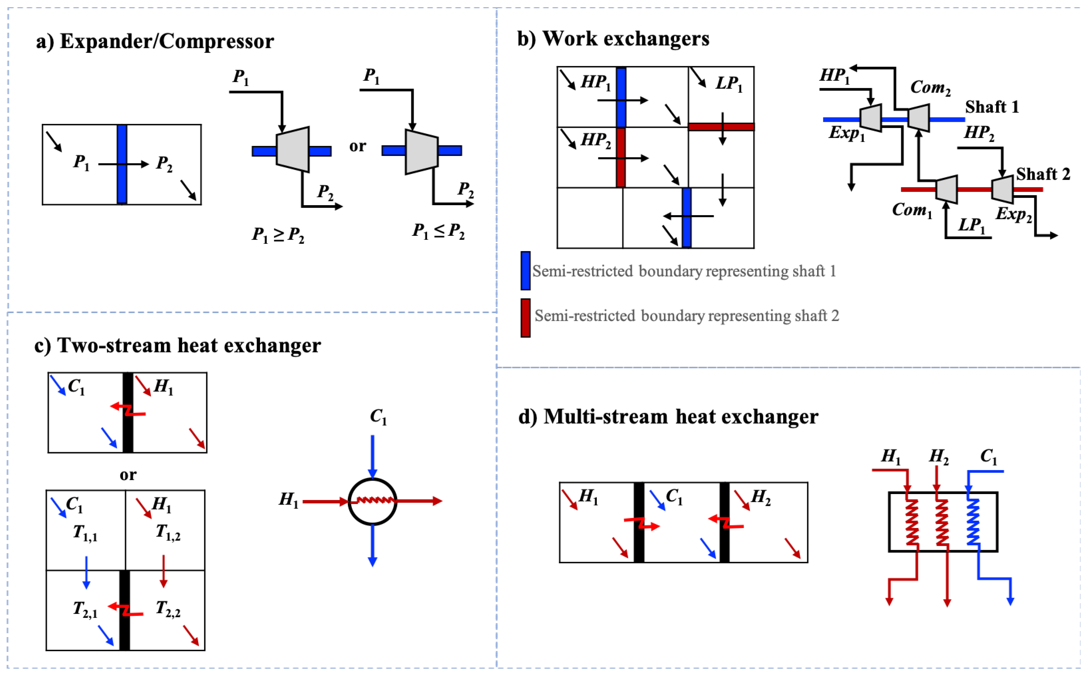
For example, Figure 2a shows a block representation and its corresponding flowsheet configuration of an operation involving a single stream undergoing a pressure change. The block representation is given by two blocks and , separated by a semi-restricted (blue) boundary. (From now on, will represent a block placed in row i and column j). The stream with pressure is fed into block and goes through the boundary to achieve the target pressure . Depending on the inlet and outlet pressures, this boundary is assigned with an expander/valve (when ≥ ) or a compressor (when ≤ ). In Figure 2b, two high-pressure streams, (HP and HP) are integrated with a low-pressure stream (LP). These two high-pressure streams pass through two expanders and respectively to achieve the desired pressure. The pressure of stream LP is increased to the target pressure after two compressors ( and ). The corresponding block representation involves building blocks. Feed HP is supplied into block and withdrawn as product in block while feed HP is supplied into block and withdrawn as product in block . The low-pressure stream LP is fed into block and withdrawn from block . Please note that there are four semi-restricted boundaries in this block representation, which include the right boundaries of block , and and the bottom boundary of block . Specifically, the right boundaries of block and block are assigned with expanders. The bottom boundary of block and the right boundary of are assigned with compressors. The expander at right boundary of block and the compressor at the right boundary of block are sharing shaft 1 (both are marked as blue). The expander at right boundary of block and the compressor at bottom boundary of block are sharing shaft 2 (both are marked as red). For illustration purpose, the boundary between block and block is specified as unrestricted boundary, where the pressure and are the same.
In the case of heat exchange (Figure 2c), a cold stream is integrated with a hot stream through a heat exchanger. Two equivalent block representations are presented. On involves a representation with two blocks. The left block allows the entering of cold stream and produces the product stream with the desired temperature. Hot stream enters the right block and is withdrawn from the same block. This heat exchanger is represented through a completely restricted boundary between block and . The energy flow is transferred from block to block . Another representation involves more blocks but better captures the relation of temperature change. Cold stream enters block with inlet temperature as and flows into block with target temperature as . Hot stream enters block with inlet temperature as and is withdrawn from block with temperature as . The right boundary of block is a completely restricted boundary. As shown in Figure 2d, a block with multiple completely restricted boundary can represent an MHEX. The cold stream enters block and takes heat from hot stream in block and from hot stream in block .
2.3. Flowsheet Representation
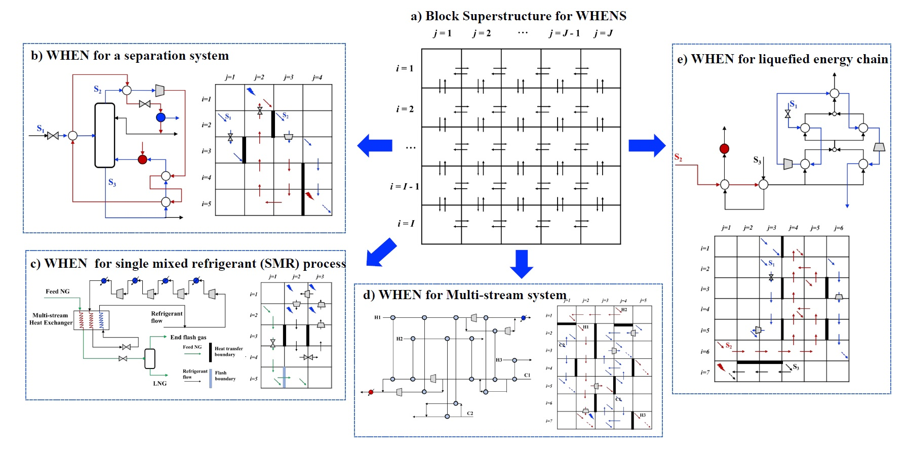
As we add more blocks in the 2-D grid assembly, we enlarge the space for representing more and more equipment and flowsheet alternatives in a single structure. The versatility of the block representation can be seen in Figure 3, where blocks are used to represent WHENS superstructures taken from a range of literature problems such as separation system for propane and propylene [24], liquefied energy chain [24,29], general work and heat integration process [13], and single mixed refrigerant (SMR) process [45]. For instance, the separation system involving three process streams , and is represented by a block representation with and to involve all connectivities for work and heat integration. enters block and flows through a valve before entering block . with varying identity is supplied into block and is compressed at the bottom boundary of block . The heat transfer happens at right boundary of block between stream and stream , right boundary of between cold side of and hot side of , right boundary of between stream and and right boundary of between stream and stream .
A process with multi-stream heat exchanger is shown in Figure 3d. The natural gas (NG) feed enters block and flows into the block with its right boundary as completely restricted boundary. The NG stream goes through a valve assigned on the bottom boundary of block before entering block with a flash boundary. The details of these separation boundaries can be found in Li et al. [38] Refrigerant flow enters block and undergoes sequential compression and cooling in block , , and . The outlet stream from block serves as a hot stream, supplying heat to the same stream after valve operation at the right boundary of block . The MHEX is represented by a block, i.e., with two completely restricted boundary. Based on the representation approach, we develop the corresponding MINLP model for WHENS, which is discussed in the next section.
2.4. Block Superstructure for WHENS
As shown in Figure 2 and Figure 3, the block representation indicates towards a unified approach for WHENS while accounting for the interplay of pressure and temperature. As we infer more, a generalized two-dimensional grid-like orientation of building blocks can be used to contain numerous flowsheet configurations for simultaneous heat and work integration. To this end, our block-based WHENS superstructure is shown in Figure 4. This representation consists of building blocks arranged in a grid with I number of rows and J number of columns. Feed f with component flowrate as and product streams p with component flowrate as are potentially supplied into or withdrawn from block . Each block has temperature and pressure attributes as and . These blocks are connected to each other through adjacent connecting streams and jump connecting streams (see black arrows and gray arrows in Figure 4a respectively).
Each adjacent connecting stream has both positive and negative components as and to allow more network alternatives. designates the flow from block to block in horizontal direction ( ) or the flow from block to block in vertical direction (). designates the flow from block to block in horizontal direction ( ) or the flow from block to block in vertical direction (). Besides, jump flow from block to block with component flowrate as is introduced to avoid unnecessary intermediate blocks for transferring material and energy flow, where and designate the row and column position of a different block in the block superstructure.
Adjacent blocks are separated via unrestricted, semi-restricted or completely restricted boundary. Both unrestricted and semi-restricted boundaries allow mass and energy flow. The thermodynamic driving force at these boundaries enables the changes of temperature and pressure. Unrestricted boundary allows mass and energy flow while ensuring the inlet pressure equal to outlet pressure, i.e., the block pressure in adjacent blocks separated by unrestricted boundary are the same. Semi-restricted boundary allows pressure change between adjacent blocks and hence indicates the existence of a pressure exchanger, i.e., compressors, expanders, or valves (shown in Figure 4b gray box). Completely restricted boundary prohibits mass flow while allowing energy flow (shown in Figure 4b black box). The existence of completely restricted boundary indicates a heat exchanger between two streams in the adjacent blocks. When a block includes more than one completely restricted boundaries, this block can be regarded as an MHEX. The inlet pressure for pressure exchangers are when the adjacent connecting streams across the semi-restricted boundary are outlet flow from block . The outlet pressure for these pressure exchangers are in horizontal direction and in vertical direction when is coming out from block . The block temperature is the temperature of outlet streams from block . With the block temperature and pressure , the unit enthalpy in block for component k can be determined. In addition to the heat transfer happening at completely restricted boundary, each block also allows external utility stream to supply extra heat duty or cold duty .
3. MINLP Model for WHENS
We now present an MINLP model for WHENS using building block-based superstructure. The overall problem is described as follows. When given a set of inlet process streams with temperature and pressure specifications as and , and a set of outlet process streams with target temperature and pressure ranges as [, ] and [, ], respectively, synthesize the optimal work and heat exchanger network that minimizes the total annual cost. The MINLP model will involve block material and energy balances, flow directions, work calculations, phase relations, boundary and task assignments, and logic constraints. The known flowrates of inlet process streams is designated as . The objective is to synthesize a work and heat exchanger network that captures the interplay of pressure and temperature to minimize the total annual cost. The set designates the flow alignment. The flow alignment when the stream is flowing in the horizontal direction, i.e., from block to ; when the stream is flowing in the vertical direction, i.e., from block to . The temperature range and flowrate range for all connecting flows including direct connecting flow and jump connecting flow is set as [, ] and [, ] respectively. The assumptions for this work are continuous steady-state operation, adiabatic expansion/compression, and linear relation of stream enthalpy with pressure and temperature. With these, we now describe the MINLP model for WHENS based on block superstructure.
3.1. Block Material Balance
The generic material balance is imposed on each individual block. The inlet flow for component k at block includes horizontal inlet flow , vertical inlet flow , external feed stream , and inlet stream via jump flow . The outlet flow for component k at block includes the horizontal outlet flow , vertical outlet flow , external product stream and outlet stream via jump flow .
We set to avoid other interactions between the superstructure and the environment except those through external feeds and products. External feed stream of component k, , collect the component flowrate, , from all available feed f. External product stream is the summation of component flowrate, , from all possible product stream p in block . Similarly, and are determined from the jump connecting flow . These are achieved through the following constraints.
Here the set collects all jump connectivities from block to block .
We define a feed fraction variable for feed stream f in block . Therefore, the component flowrate through feed f into block , can be determined as follows:
where is the maximum available amount of feed stream f. is composition of component k in feed f. Summation of these feed fraction variables will be less than 1 if the overall feed amount is less than .
The flowrate range for product stream p is restricted from minimum product flowrate to maximum product flowrate .
In general, the flowrate range for product stream p is equal to inlet flowrate, indicating .
3.2. Flow Directions
We consider the connecting stream between adjacent blocks as a bidirectional flow. Its positive and negative components are and respectively. The selection of flow direction is achieved through the following binary variable:
The following constraints ensure that only one component of this connecting stream is activated:
Besides, with these stream components, the overall inlet flow is the summation of all incoming streams into block :
3.3. Block Energy Balance
The block energy balance includes stream enthalpy, feed enthalpy, product enthalpy, external heating/cooling, work energy associated with expansion/compression and contacting energy flow across the block boundary. Then the steady-state energy balance for block is formulated as follows:
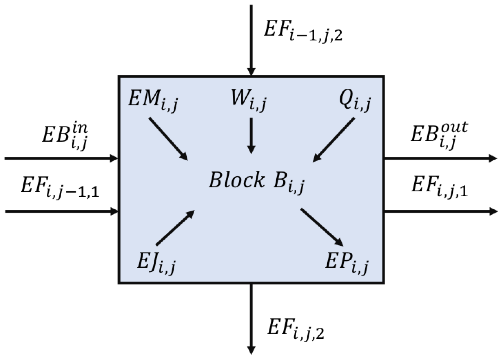
where , and are inlet enthalpy and outlet enthalpy streams to block respectively. is the overall stream enthalpy carried by feed streams. is the overall product enthalpy carried by product streams. is the enthalpy supplied by utility streams into block . is the work energy supplied through compression operation or expansion operation for block respectively. Besides, is the stream enthalpy carried along with the jump connecting streams. represents the energy flow going through the completely restricted boundary and indicates the amount of heat transfer between adjacent streams. These energy flow variables are shown in Figure 5.
The inlet stream enthalpy to block consists of inlet stream enthalpy from adjacent blocks in horizontal directions, i.e., and , stream enthalpy from adjacent blocks in vertical directions, i.e., and , and stream enthalpy through inlet jump connecting streams, i.e., . Hence, is determined as follows:
Similarly, the outlet stream enthalpy to block , is determined as follows:
These stream enthalpies are determined based on the flowrate and the unit enthalpy. For outlet streams from block in flow alignment d, the initial unit enthalpy for these streams are the block enthalpy . For the inlet stream to block in horizontal direction with flow alignment , the initial unit enthalpy is the unit enthalpy in block . For the inlet stream to block in vertical direction with flow alignment , the initial unit enthalpy is the enthalpy in block .
The feed stream enthalpy in block is based on the flowrate of feed streams and stream enthalpy of feed streams .
is a parameter determined by the feed temperature and pressure.
The product stream enthalpy from block is based on the flowrate of product streams and stream enthalpy in this block.
The utility enthalpy term consists of hot utility, and cold utility , which are supplied into block .
To obtain the fixed cost of heaters and coolers, we define the following two binary variables:
It is straightforward to relate heat duty of heaters and coolers with these two binary variables:
Here is the upper bound of stream enthalpy.
The work energy is determined by the amount of work added into or taken out of block , which are denoted as for compression and for expansion, respectively. The calculation of and is explained later in this Section 3.8.
The stream enthalpy across the completely restricted boundary is either in the positive direction () or in the negative direction ().
3.4. Product Stream Assignments and Logical Constraints
We define binary variables for each product stream p at block to determine whether they are active in or not:
The identification of block as product block is achieved through the following logical relation, which involves product binary variable.
For each block, there are at most one type of product stream present in block . The logic proposition is illustrated as follows:
At least one stream for product p appears in the block superstructure.
The temperature range for block with product stream p is , .
Likewise, the pressure range for product block is , as follows.
We impose the following constraint to tighten the bounds of block pressure for blocks not involving product streams. This constraint states that if the block includes component k, then the block pressure is larger than the minimum product pressure .
Here, the set specifies the type of component k in product p.
Similarly, if the block includes component k, then the block temperature is correspondingly bounded above the minimum product temperature .
In WHENS problem, we assume mixing of different streams. Hence, we define the following binary variable to decide which component is allowed to exist in block .
The following constraints ensure that at most one component is allowed in block and all other inlet component streams are prohibited from entering this block.
If the block supplies product stream p, the required component k should exists in this block. Similarly, if the block takes feed stream f, the feed components k are inside the same block.
Here the set specifies all components k in feed f.
The existence of component k in block facilitate the tightening the bounds of block temperature .
Here and are maximum and minimum temperature in the system with and
3.5. Boundary Assignment
The block boundaries are assigned as either unrestricted, semi-restricted or completely restricted boundary. If there is no pressure change across adjacent blocks through their connecting streams, then the inter-block boundary is unrestricted. If there is pressure change across a boundary, then the boundary is semi-restricted. If there is no mass allowed to flow between adjacent blocks, then the inter-block boundary is identified as completely restricted boundary.
Only one type of the boundaries is activated between two adjacent blocks.
Mass flow is prohibited while energy flow is allowed across a completely restricted boundary between adjacent blocks.
3.6. Phase Relation and Stream Enthalpies
Each block has phase assignment according to the components existing in it, temperature, and pressure condition. We define binary variables for liquid phase and gas phase in block . This phase relations are adapted from the work of Nair et al. [24].
Besides the following 0–1 continuous variable is defined for the two-phase zone in block .
The enthalpy expression for liquid phase and gas phase is linearly dependent on the block temperature and block pressure .
Here , , , , and are parameters used for determining the enthalpy of liquid and gas phase.
The enthalpy expression for two-phase region is approximated as the linear segment between enthalpy at bubble point and that at dew point .
The bubble point and dew point for component k in block are linearly dependent on the block pressure .
Here , , , and are parameters for determining bubble point and dew point.
The general bubble point and dew point temperatures are then assigned to block bubble temperature and block dew temperature , if component k exists in block .
The definition of is achieved through the following constraint.
When and , the above constraint is reduced to .
Block temperature is related with and respectively through the following two constraints.
Similarly, the obtained enthalpy expressions , , and map to the block enthalpy via , , and through the following big-M constraints.
Here , , , and are appropriate big-M values.
3.7. Heat Transfer Boundary Modeling
Instead of following the conventional heat integration [46], we propose a heat transfer boundary model. The representation for model describes the heat transfer across a wall (completely restricted boundary). The block that supplies the energy flow is the heat source, while the block that takes the energy flow is the heat sink. Hence, there is no need to assign binary variable for determining the identity of process streams in each block since they are automatically determined by the heat transfer direction. Besides, no stage number for heat integration need to be specified in advance.
The total amount of heat duty exchanged at boundary between block and in horizontal direction (or between block and in vertical direction) is determined as follows:
The inlet temperature to block is designated . The bound of can be tightened to be if component k exists in block . This is achieved through the following constraint:
The inlet temperature to block , , is equal to the temperature of overall inlet streams after mixing effect. The is obtained through the following energy balance at the inlet port of the block . Since compression or expansion operation also contribute to the temperature change at the inlet part of each block, and are included into the energy balance at the inlet port.
The inlet stream enthalpy terms on the right-hand side of the above equation is determined based on the inlet temperature of the destinate block , the pressure of the destinate block (since and already contributes to the pressure change).
The phase of the above streams, , , , , and , are the same as the phase of block where these streams originate from. Parameter describes the phase of feed streams, which is equal to one if feed enters the system as gas and equal to zero if the feed enters the system as liquid.
When the energy flow direction in horizontal direction is from block to block (), the inlet and outlet approach temperatures for process streams in adjacent blocks separated by completely restricted boundary are determined as follows:
Here when energy flow direction is in positive direction and . The inlet approach temperature and outlet approach temperature are and .
Similarly, the approach temperatures for process streams exchanging heat in vertical direction () are determined as follows:
When the energy flow direction in horizontal direction is from block to block , the inlet and outlet approach temperatures are obtained with the following two relations:
Similarly, in vertical direction () with energy flow direction from block to block , the inlet and outlet approach temperatures are obtained with the following two relations:
Similarly, approach temperatures for blocks with hot utility and cold utility are given by:
Parameters and are outlet and inlet temperature of cold utility while and are outlet and inlet temperature of hot utility.
Only one heat duty at heat transfer boundary and one approach temperature variable are required for determining the heat exchanger area. These are ensured through the following inequalities:
With the approach temperature and heat duty of heat exchangers, we determine the heat exchange areas as follows:
Here, , and represent heat exchange area between process streams, between process stream in block and hot utility, between process stream in block and cold utility respectively. We use Chen’s approximation to calculate the logarithmic mean temperature difference in area calculations. , , are overall heat transfer coefficient at heat exchangers, heaters, and coolers.
3.8. Work Calculation
A semi-restricted boundary can be assigned with either an expander, a compressor, or a valve. These assignments are indicated through the following binary variables:
Only one of these pieces of pressure-changing equipment is allowed on semi-restricted boundary.
For the right or bottom boundary of block ( or ), there can be a situation that while the flow associated with the boundary . This does not indicate an existence of valve operation at the boundary but suggests that the temperature and pressure relation at the boundary is relaxed. This avoids the happening of infeasibility. Since is also not related with the cost function, its value has no influence on the objective value.
The existence of shaft m is indicated through the following binary variable:
If an SSTC exists, there is at least one compressor or turbine. To avoid symmetric solution, we prefer shaft with lower index.
On each shaft, there exists a motor or a generator. These are represented with binary variables:
If a shaft does not exist, then the motor and generator on this shaft also do not exist. If a generator or a motor exists on a shaft, then there is at least one semi-restricted boundary assigned with turbines or compressors on this shaft.
We define the positive variable to designate the pressure ratio between the block and for flow alignment or between the block and for flow alignment . The calculation of is activated when the boundary of block is semi-restricted or unrestricted at the corresponding flow alignment d ( = 1 or = 1). The pressure ratio is taken as 1 to avoid the calculation of the pressure ratio if this boundary is not semi-restricted. In horizontal direction, the pressure ratio is determined as follows:
Here, is taken as the maximum pressure ratio, which is determined as . Similarly, in vertical direction, the pressure ratio is determined as follows:
For feed stream f, the pressure ratio is taken as the ratio between block pressure and parameter for feed pressure .
The work term consists of compression work term and expansion work term . Both and consist of work components for direct connecting streams ( for positive component, for negative component), feed streams(), and jump connecting streams (). Accordingly,
From these pressure ratio definitions, we calculate the isentropic work on direct connecting streams, feed streams and jump connecting streams. In the horizontal direction, the inlet isentropic work is determined as follows:
Here is the gas constant and is the adiabatic compression coefficient. is the adiabatic compression efficiency. Similarly, the isentropic work for a vertical entering stream is calculated as follows:
The work terms related to feed streams and jump connecting streams are calculated in a similar way:
Here is the adiabatic compression coefficient.
These work components for direct connecting streams are related with the boundary type and the type of pressure exchangers assigned on semi-restricted boundary.
The compression work energy and expansion energy are determined as follows:
The following shaft balance distributes the energy generated by turbines to compressors on the same shaft. Additional energy is transferred to motors to generate electricity. If the energy supply is not enough, electricity is consumed to activate motors.
and designate the maximum capacity of motors and generators, respectively. Please note that valves do not contribute to work energy. Hence, whenever the semi-restricted boundary is assigned with a valve, then that work energy term is ignored.
Additional constraints ensure that the block assigned with turbines or compressors should involve with gas phase.
3.9. Objective Function
We consider an economic objective similar to Nair et al. [24] as follows:
Here is the annualized factor. This objective function aims at minimizing total annual cost (). This mainly involves capital costs including those of generator, motor, compressor, expander, and heat exchangers, as well as operating cost including costs of running motors, utility consumption. Besides, the electricity generated by generators bring revenue. The parameter is the fixed cost for different equipment. is the appropriate cost coefficient for associated equipment. is the unit cost for utilities. is the price of electricity while parameter is the cost factor.
4. WHENS Case Study on Liquefied Natural Gas (LNG)-Based Cryogenic Energy Chain
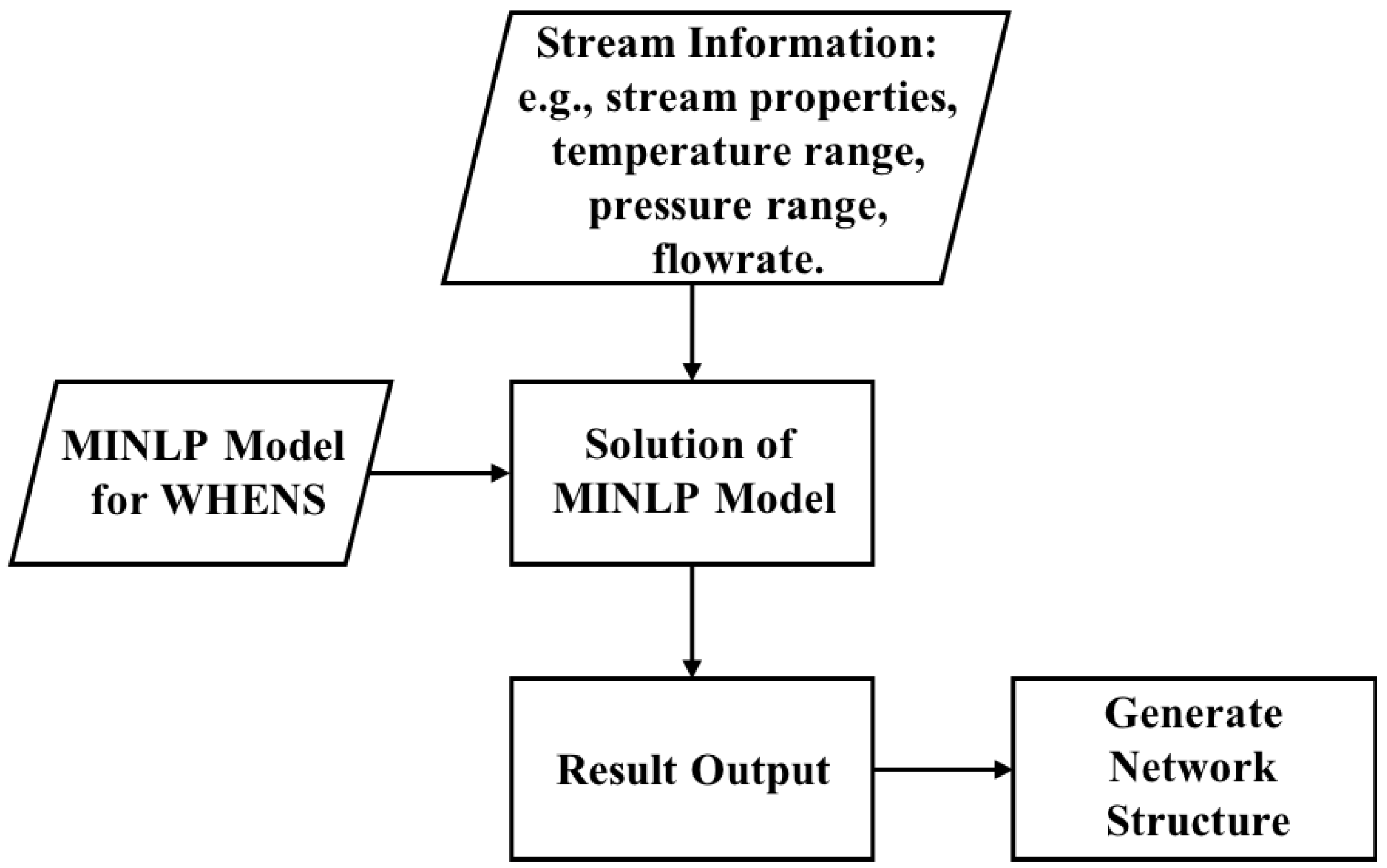
The above MINLP model is applied to a WHENS problem related to a liquefied energy chain reported by Nair et al. [24]. Liquefaction is an energy-intensive process that converts natural gas (NG) into liquid form for economic and safe transportation [47,48,49]. The overall procedure for solving the case study is illustrated in Figure 6.
The stream information such as stream properties, temperature range, pressure range, and flowrate is directed to the block-based MINLP model for WHENS problem. This MINLP is solved using commercial solvers and results in block configurations. The block configurations are then converted to classic work and heat exchange networks. The procedure for this conversion can be found in Demirel et al. [37] and Li et al. [38] There are four process streams, including liquid inert nitrogen (), liquefied natural gas or LNG (), liquid carbon dioxide (), and the propane pre-cooled mixed refrigerant (C3MR) () and one external stream as hot utility (HU). Among these process streams, part of also serves as cold utility stream (CU). The information is provided in Table 2.
Stream property information is provided in Table 3 and include bubble point, dew point, enthalpy calculation for streams in liquid and gas phases. Since we assume these variables are linearly dependent on both system temperature and pressure, the following linear coefficients are sufficient to capture the thermodynamic relations. The unit for bubble point and dew point are K while the units for liquid enthalpy and gas enthalpy are kJ/kg.
The equipment considered are compressors, expanders, motors, generators, and heat exchangers. The cost coefficients for them are reported in the Table 4. Please note that the additional amount of energy brought by generator can be converted into electricity, contributing to the revenue gaining.
We select a block superstructure. To facilitate the solution, we reduce the number of binary variables by prohibiting the use of valves. The heat transfer boundaries are only allowed in the horizontal direction. To reduce the number of non-linear terms, we fix all jump connecting streams to be zero. This restricts the number of process alternatives but helps to demonstrate the capability of the proposed approach. This case study is solved using solver ANTIGONE 24.4.3 developed by Misener et al. [50] in GAMS 24.4 (2015 version and developed by GAMS Development Corporation in Fairfax, VA, USA) on a Dell OptiPlex 9020 computer (Intel 8 Core i7-4770 CPU 3.4 GHz, 15.5 GB memory) running Springdale Linux. We consider two different cases of this case study to show the capability of the proposed approach. Case 1 involves liquefaction of NG using available process streams. Case 2 achieves the liquefaction of NG using C3MR.
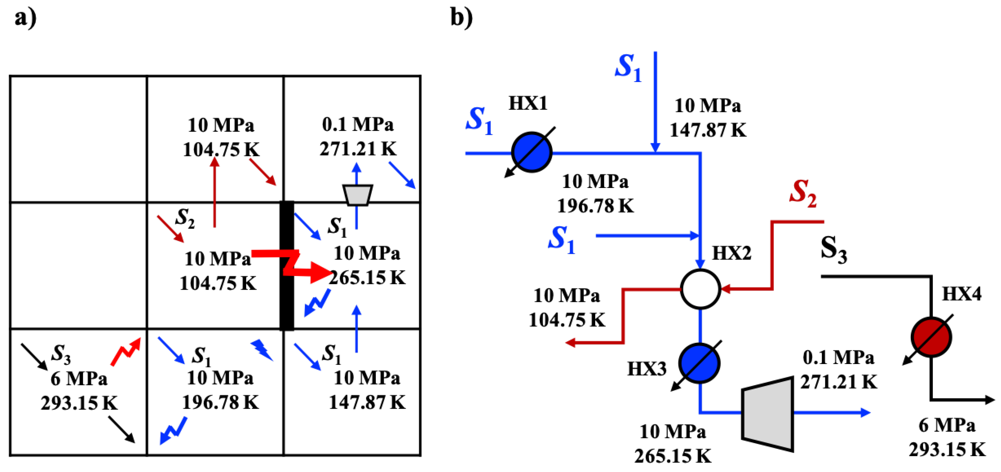
Solver SCIP (representing Solving Constraint Integer Programs) [51] is used for initializing the proposed model. This model is solved within 2 h with optimal total annual cost as 0.696 MM$/year with total capital cost of 0.225 MM$/year and operating cost of 0.471 MM$/year. The block configuration and the equivalent process flowsheet are shown in Figure 7. Stream flows into block and is cooled using the HU. Stream is distributed in block , block and block with feed fractions of 0.34, 0.18, and 0.32, respectively. A CU is supplied into block to partially cool down the stream . The vertical outlet flow of block is integrated with stream , where serves as the hot stream and in block serves as the cold stream. Please note that the identity of these two streams were not postulated in advance. This was identified by the heat transfer direction reported in the solution. For instance, the energy flow at the right boundary of block is from block to block . Hence, the stream in block is a hot stream while the stream in block is a cold stream. The additional amount of heat transferred from block is compensated by a CU in block . After heat integration, stream is withdrawn in block and stream is withdrawn in block after the expansion at the bottom boundary of block . The relevant block temperature and block pressure can be found in Figure 7a.
The corresponding process flowsheet is shown in Figure 7b. Streams and are integrated through heat exchanger HX2 with heat duty of 862.61 KW. Stream is not involved in either heat integration or work integration. A heater with heat duty as 410.74 KW helps stream to achieve the design target. The heat duty of coolers on stream are 10.42 KW, 381.36 KW for cooler HX1 and HX3, respectively. Through this case study on liquefied energy chain, we show that the proposed approach could enable both heat and work integration opportunities. These integration alternatives reduced the energy consumption and total annual cost, resulting in significant energy intensification within the network structure. The identity of process streams was determined simultaneously together with network generation. Besides, compared with classic superstructure representation approach, no information on work and heat exchange stage number was required.
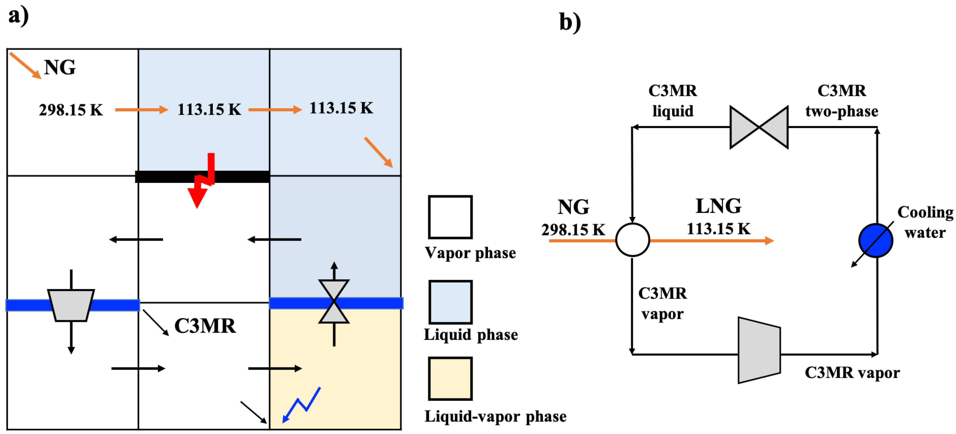
Next, we consider a conceptual design problem where the goal is to obtain a liquefaction process for a NG stream from an initial gaseous condition of 1 atm and 298.15 K to a final condition of saturated LNG at 1 atm (which corresponds to a final temperature below 113.15 K). Interestingly, this process synthesis problem can be formulated as a WHENS problem, where we have two process streams, namely the NG (hot stream) and C3MR. The refrigerant can be considered as a neutral stream or a circulating working fluid with the same initial and final conditions. Any feasible process configuration for this design problem would involve heat exchangers, and the temperatures indicate that cryogenic cooling is necessary. However, consider that cooling water at the ambient temperature is the only CU that is available for the process. To this end, work exchangers (compressors and expanders) would be required. The refrigerant would undergo a cycle involving multiple alternating heat and work exchangers to first achieve a cryogenic temperature through expansion at which heat can be gained from the NG stream, and then achieve a high temperature through compression at which heat can be released to the cooling water. This is what happens in a typical refrigeration cycle.
While such an answer is well-known for this problem, this is to illustrate the possibility of discovering non-intuitive process flowsheets involving heat and work exchangers using the building block approach. Consider a naive designer who does not have any prior knowledge of how a refrigeration cycle works, or how a stream should be liquefied at cryogenic conditions when cooling utilities are only available at the ambient condition. The designer can still obtain the same solution, as it is already embedded in the general block-based WHENS superstructure (see Figure 8).
The NG stream enters the process as a gaseous stream in block and finally exits as a saturated liquid from block . Before exiting, NG exchanges heat with the refrigerant C3MR through the bottom boundary of block . C3MR cycles through the blocks placed in rows 2 and 3. Starting from block , the refrigerant C3MR enters as a vapor stream and is cooled into a two-phase mixture in a utility cooler using cooling water as the CU. The outlet stream from block is expanded which results in a liquid C3MR with a reduced temperature when entering the block through a valve placed at the top semi-restricted boundary of block . The horizontal outlet stream of block is vaporized using the heat released by NG through the completely restricted boundary between the blocks and . The C3MR vapor after the heat exchanger is compressed across a semi-restricted boundary assigned on the bottom of block before it is finally withdrawn in block . The seamless entrance and exit of C3MR within the same block suggests the existence of a cycle. The corresponding process flowsheet is shown in Figure 8b.
5. Conclusions
We presented a method to automatically generate numerous alternative configurations for the synthesis of integrated work and heat exchange networks using building blocks. The block representation is abstract, and it requires a transformation to obtain classic unit operations and flowsheet configurations. However, it is also analogous in a sense that the transformations from blocks-to-flowsheets and from flowsheets-to-blocks are systematic. The benefits of block-based representation over a unit operations-based representation is that the former uses only two fundamental design elements, namely the block interior and the block boundary. Alternative arrangement of flows to block interior and assignment of work/heat transfer phenomena to block boundaries give rise to alternative networks for systematic WHENS. The heat and work transfer models are general such that they do not depend on the postulation of stream identities. Besides, there is no need to specify any stagewise integration. With this representation approach, we formulated an MINLP model for WHENS. Using a case study, we demonstrated the capability of the block-based approach for WHENS. We also considered the possibility of discovering non-intuitive process flowsheets involving heat and work exchangers. Specifically, the case of NG liquefaction indicated that a designer could generate the design of a refrigeration cycle using the building block approach, even when designers have no prior knowledge of how a refrigeration cycle works, or how a stream should be liquefied at cryogenic conditions when cooling utilities are only available at ambient conditions. This provides hints towards the potential of our approach for the discovery of novel processes through process synthesis. However, further research is needed to extend the simultaneous process synthesis along with work and heat integration to more complex scenarios.
Author Contributions
J.L., S.E.D., and M.M.F.H. conceived the ideas, models and prepared the manuscript.
Funding
The authors gratefully acknowledge financial support from the U.S. National Science Foundation (NSF CBET-1606027) and the DOE/RAPID NNMI Institute.
Conflicts of Interest
The authors declare no conflict of interest.
References
- Yu, H.; Fu, C.; Vikse, M.; Gundersen, T. Work and heat integration—A new field in process synthesis and PSE. AIChE J. 2018. [Google Scholar] [CrossRef]
- Fu, C.; Vikse, M.; Gundersen, T. Work and heat integration: An emerging research area. Energy 2018, 158, 796–806. [Google Scholar] [CrossRef]
- Huang, K.; Karimi, I. Work-heat exchanger network synthesis (WHENS). Energy 2016, 113, 1006–1017. [Google Scholar] [CrossRef]
- Subramanian, A.; Gundersen, T.; Adams, T.A., II. Modeling and simulation of energy systems: A Review. Processes 2018, 6, 238. [Google Scholar] [CrossRef]
- Furman, K.C.; Sahinidis, N.V. A critical review and annotated bibliography for heat exchanger network synthesis in the 20th century. Ind. Eng. Chem. Res. 2002, 41, 2335–2370. [Google Scholar] [CrossRef]
- Huang, Y.; Fan, L. Analysis of a work exchanger network. Ind. Eng. Chem. Res. 1996, 35, 3528–3538. [Google Scholar] [CrossRef]
- Razib, M.; Hasan, M.M.F.; Karimi, I.A. Preliminary synthesis of work exchange networks. Comput. Chem. Eng. 2012, 37, 262–277. [Google Scholar] [CrossRef]
- Liu, G.; Zhou, H.; Shen, R.; Feng, X. A graphical method for integrating work exchange network. Appl. Energy 2014, 114, 588–599. [Google Scholar] [CrossRef]
- Zhuang, Y.; Liu, L.; Zhang, L.; Du, J. Upgraded graphical method for the synthesis of direct work exchanger networks. Ind. Eng. Chem. Res. 2017, 56, 14304–14315. [Google Scholar] [CrossRef]
- Zhuang, Y.; Liu, L.; Du, J. Direct Work Exchange Networks Synthesis of Isothermal Process Based on Superstructure Method. Chem. Eng. Trans. 2017, 61, 133–138. [Google Scholar]
- Amini-Rankouhi, A.; Huang, Y. Prediction of maximum recoverable mechanical energy via work integration: A thermodynamic modeling and analysis approach. AIChE J. 2017, 63, 4814–4826. [Google Scholar] [CrossRef]
- Fu, C.; Gundersen, T. Heat and work integration: Fundamental insights and applications to carbon dioxide capture processes. Energy Convers. Manag. 2016, 121, 36–48. [Google Scholar] [CrossRef]
- Fu, C.; Gundersen, T. Correct integration of compressors and expanders in above ambient heat exchanger networks. Energy 2016, 116, 1282–1293. [Google Scholar] [CrossRef]
- Fu, C.; Gundersen, T. Integrating compressors into heat exchanger networks above ambient temperature. AIChE J. 2015, 61, 3770–3785. [Google Scholar] [CrossRef]
- Fu, C.; Gundersen, T. Integrating expanders into heat exchanger networks above ambient temperature. AIChE J. 2015, 61, 3404–3422. [Google Scholar] [CrossRef]
- Fu, C.; Gundersen, T. Sub-ambient heat exchanger network design including compressors. Chem. Eng. Sci. 2015, 137, 631–645. [Google Scholar] [CrossRef]
- Aspelund, A.; Berstad, D.O.; Gundersen, T. An extended pinch analysis and design procedure utilizing pressure based exergy for subambient cooling. Appl. Therm. Eng. 2007, 27, 2633–2649. [Google Scholar] [CrossRef]
- Gundersen, T.; Berstad, D.O.; Aspelund, A. Extending pinch analysis and process integration into pressure and fluid phase considerations. Chem. Eng. Trans. 2009, 18, 33–38. [Google Scholar]
- Kansha, Y.; Tsuru, N.; Sato, K.; Fushimi, C.; Tsutsumi, A. Self-heat recuperation technology for energy saving in chemical processes. Ind. Eng. Chem. Res. 2009, 48, 7682–7686. [Google Scholar] [CrossRef]
- Tsutsumi, A.; Kansha, Y. Thermodynamic mechanism of self-heat recuperative and self-heat recovery heat circulation system for a continuous heating and cooling gas cycle process. Chem. Eng. Trans. 2017, 61, 1759–1764. [Google Scholar]
- Dong, R.; Yu, Y.; Zhang, Z. Simultaneous optimization of integrated heat, mass and pressure exchange network using exergoeconomic method. Appl. Energy 2014, 136, 1098–1109. [Google Scholar] [CrossRef]
- Onishi, V.C.; Ravagnani, M.A.; Caballero, J.A. Simultaneous synthesis of work exchange networks with heat integration. Chem. Eng. Sci. 2014, 112, 87–107. [Google Scholar] [CrossRef] [Green Version]
- Vikse, M.; Fu, C.; Barton, P.I.; Gundersen, T. Towards the use of mathematical optimization for work and heat exchange networks. Chem. Eng. Trans. 2017, 61, 1351–1356. [Google Scholar]
- Nair, S.K.; Nagesh Rao, H.; Karimi, I.A. Framework for work-heat exchange network synthesis (WHENS). AIChE J. 2018, 61, 871–876. [Google Scholar] [CrossRef]
- Floudas, C.A.; Ciric, A.R.; Grossmann, I.E. Automatic synthesis of optimum heat exchanger network configurations. AIChE J. 1986, 32, 276–290. [Google Scholar] [CrossRef]
- Yeomans, H.; Grossmann, I.E. A systematic modeling framework of superstructure optimization in process synthesis. Comput. Chem. Eng. 1999, 23, 709–731. [Google Scholar] [CrossRef]
- Chen, Q.; Grossmann, I. Recent developments and challenges in optimization-based process synthesis. Annu. Rev. Chem. Biomol. Eng. 2017, 8, 249–283. [Google Scholar] [CrossRef] [PubMed]
- Demirel, S.E.; Li, J.; Hasan, M.M.F. Systematic process intensification. Curr. Opin. Chem. Eng. 2019, in press. [Google Scholar]
- Wechsung, A.; Aspelund, A.; Gundersen, T.; Barton, P.I. Synthesis of heat exchanger networks at subambient conditions with compression and expansion of process streams. AIChE J. 2011, 57, 2090–2108. [Google Scholar] [CrossRef]
- Uv, P.M. Optimal Design of Heat Exchanger Networks with Pressure Changes. Master’s Thesis, NTNU, Trondheim, Norway, 2016. [Google Scholar]
- Stankiewicz, A.I.; Moulijn, J.A. Process intensification: Transforming chemical engineering. Chem. Eng. Prog. 2000, 96, 22–34. [Google Scholar]
- Reay, D.; Ramshaw, C.; Harvey, A. Process Intensification: Engineering for Efficiency, Sustainability and Flexibility; Butterworth-Heinemann: Oxford, UK, 2013. [Google Scholar]
- Tian, Y.; Demirel, S.E.; Hasan, M.M.F.; Pistikopoulos, E.N. An Overview of Process Systems Engineering Approaches for Process Intensification: State of the Art. Chem. Eng. Process.-Process Intensif. 2018, 133, 160–210. [Google Scholar] [CrossRef]
- Demirel, S.E.; Li, J.; Hasan, M.M.F. A General Framework for Process Synthesis, Integration and Intensification. Comput. Aided Chem. Eng. 2018, 44, 445–450. [Google Scholar]
- Hasan, M.M.F.; Karimi, I.A.; Alfadala, H.E.; Grootjans, H. Operational modeling of multistream heat exchangers with phase changes. AIChE J. 2009, 55, 150–171. [Google Scholar] [CrossRef]
- Nagesh Rao, H.; Karimi, I.A. A superstructure-based model for multistream heat exchanger design within flow sheet optimization. AIChE J. 2017, 63, 3764–3777. [Google Scholar] [CrossRef]
- Demirel, S.E.; Li, J.; Hasan, M.M.F. Systematic process intensification using building blocks. Comput. Chem. Eng. 2017, 105, 2–38. [Google Scholar] [CrossRef]
- Li, J.; Demirel, S.E.; Hasan, M.M.F. Process synthesis using block superstructure with automated flowsheet generation and optimization. AIChE J. 2018, 64, 3082–3100. [Google Scholar] [CrossRef]
- Li, J.; Demirel, S.E.; Hasan, M.M.F. Process Integration Using Block Superstructure. Ind. Eng. Chem. Res. 2018, 57, 4377–4398. [Google Scholar] [CrossRef]
- Li, J.; Demirel, S.E.; Hasan, M.M.F. Fuel Gas Network Synthesis Using Block Superstructure. Processes 2018, 6, 23. [Google Scholar] [CrossRef]
- Onishi, V.C.; Ravagnani, M.A.; Caballero, J.A. Simultaneous synthesis of heat exchanger networks with pressure recovery: optimal integration between heat and work. AIChE J. 2014, 60, 893–908. [Google Scholar] [CrossRef]
- Fu, C.; Gundersen, T. Sub-ambient heat exchanger network design including expanders. Chem. Eng. Sci. 2015, 138, 712–729. [Google Scholar] [CrossRef]
- Onishi, V.C.; Ravagnani, M.A.; Jiménez, L.; Caballero, J.A. Multi-objective synthesis of work and heat exchange networks: Optimal balance between economic and environmental performance. Energy Convers. Manag. 2017, 140, 192–202. [Google Scholar] [CrossRef]
- Zhuang, Y.; Liu, L.; Liu, Q.; Du, J. Step-wise synthesis of work exchange networks involving heat integration based on the transshipment model. Chin. J. Chem. Eng. 2017, 25, 1052–1060. [Google Scholar] [CrossRef]
- Qadeer, K.; Qyyum, M.A.; Lee, M. Krill-herd-based investigation for energy saving opportunities in offshore LNG processes. Ind. Eng. Chem. Res. 2018, 57, 14162–14172. [Google Scholar] [CrossRef]
- Yee, T.F.; Grossmann, I.E. Simultaneous optimization models for heat integration—II. Heat exchanger network synthesis. Comput. Chem. Eng. 1990, 14, 1165–1184. [Google Scholar] [CrossRef]
- Lim, W.; Choi, K.; Moon, I. Current status and perspectives of liquefied natural gas (LNG) plant design. Ind. Eng. Chem. Res. 2013, 52, 3065–3088. [Google Scholar] [CrossRef]
- Vikse, M.; Watson, H.; Gundersen, T.; Barton, P. Simulation of Dual Mixed Refrigerant Natural Gas Liquefaction Processes Using a Nonsmooth Framework. Processes 2018, 6, 193. [Google Scholar] [CrossRef]
- Kazda, K.; Li, X. Approximating nonlinear relationships for optimal operation of natural gas transport networks. Processes 2018, 6, 198. [Google Scholar] [CrossRef]
- Misener, R.; Floudas, C.A. ANTIGONE: Algorithms for continuous/integer global optimization of nonlinear equations. J. Glob. Optim. 2014, 59, 503–526. [Google Scholar] [CrossRef]
- Achterberg, T. SCIP: Solving constraint integer programs. Math. Program, Comput, 2009, 1, 1–41. [Google Scholar] [CrossRef]
Figure 1.
Elements of abstract building blocks: (a) block interior (b) block boundary.

Figure 2.
Equipment representations using building blocks for work and heat exchanger network: (a) Expander/compressor; (b) Work-exchanger shafts for work integration; (c) Two-stream exchanger for heat integration; (d) Multi-stream heat exchanger (MHEX).
Figure 2.
Equipment representations using building blocks for work and heat exchanger network: (a) Expander/compressor; (b) Work-exchanger shafts for work integration; (c) Two-stream exchanger for heat integration; (d) Multi-stream heat exchanger (MHEX).

Figure 3.
Various flowsheets and networks representations for work and heat integration in WHENS: (a) Work and heat exchange network for a separation system. (b) Work and heat exchange network for liquefied energy chain. (c) Work and heat exchange network with three hot streams and two cold streams. (d) Work and heat exchange network for single mixed refrigerant (SMR) process.

Figure 4.
A general superstructure representation using building blocks for work and heat integration in WHENS: (a) General block representation; (b) Interaction of blocks through boundaries and connecting flows.
Figure 4.
A general superstructure representation using building blocks for work and heat integration in WHENS: (a) General block representation; (b) Interaction of blocks through boundaries and connecting flows.

Figure 5.
Illustration of energy balance on block .

Figure 6.
Procedure for block-based WHENS.

Figure 7.
Resultant integrated work and heat exchanger network for the liquefied energy chain (case 1): (a) Bock representation; (b) Equivalent WHEN structure.
Figure 7.
Resultant integrated work and heat exchanger network for the liquefied energy chain (case 1): (a) Bock representation; (b) Equivalent WHEN structure.

Figure 8.
Manifestation of a refrigeration cycle using building blocks for cryogenic liquefaction process: (a) block representation, and (b) equivalent WHEN structure.
Figure 8.
Manifestation of a refrigeration cycle using building blocks for cryogenic liquefaction process: (a) block representation, and (b) equivalent WHEN structure.


Table 1.
An indicative list of recent contributions in WHENS literature.
| Reference | Approach | Application/Case Studies |
|---|---|---|
| Wechsung, Aspelund, Gundersen, Barton (2011) [29] | Combination of pinch analysis, exergy analysis, and optimization to find heat exchanger network (HEN) with minimal irreversibility by varying pressure levels of process streams | An offshore natural gas liquefaction process |
| Razib, Hasan, Karimi (2012) [7] | First formalization of an optimization-based systematic work exchange network (WEN) synthesis problem | Integration among high-pressure and low-pressure streams |
| Dong, Yu, Zhang (2014) [21] | Superstructure optimization for heat, mass and pressure exchange networks with exergoeconomic analysis | Wastewater distribution network in a petroleum refining process |
| Onishi, Ravagnani, Caballero (2014a) [41] | Superstructure optimization for HEN design with pressure recovery | Cryogenic process design |
| Onishi, Ravagnani, Caballero (2014b) [22] | MINLP-based WHENS using a multi-stage superstructure for optimal pressure recovery of process gaseous streams | Integration among high-pressure and low-pressure streams |
| Fu and Gundersen (2015a,b,c,d) [14,15,16,42] | Graphical methodology for HEN design including compressors or expanders to minimize exergy consumption above or below ambient temperature | Integration of process streams with supply and target states |
| Huang and Karimi (2016) [3] | MINLP-based approach to synthesize WHENS for optimized selection of end-heaters and end-coolers to meet the desired temperature targets | Integration among high-pressure and low-pressure streams and a transport chain for stranded natural gas |
| Fu, Gundersen (2016) [13] | Correct integration of both compressors and expanders in HEN to minimize exergy consumption | Integration of process streams with the same supply and target temperatures |
| Fu, Gundersen (2016c) [12] | Graphical methodology using thermodynamic insights for WHENS | CO capture processes |
| Onishi, Ravagnani, Caballero (2017) [43] | Multi-objective optimization of WHENS using a multi-stage superstructure | Integration among process streams based on economic and environmental criteria |
| Zhuang, Liu, Liu, Du (2017) [44] | Synthesis of direct work exchange network (WEN) in adiabatic process involving heat integration based on transshipment model | Integration of high-pressure and low-pressure streams in a chemical plant |
| Nair, Rao, Karimi (2018) [24] | MINLP-based general WHENS framework considering stream temperature, pressure and/or phase changes without a classification of stream identity | C3 splitting and offshore liquefied natural gas (LNG) processes |
Table 2.
Specification for process streams and utility streams (HU: hot utility; CU: cold utility).
| Specification/Parameter | HU | CU | ||||
|---|---|---|---|---|---|---|
| Feed pressure, (MPa) | 10 | 10 | 6 | - | - | - |
| Feed temperature, (K) | 103.45 | 319.80 (298.15) | 221.12 | - | 383.15 | 93.15 |
| Target pressure, (MPa) | 0.1 | 10 | 6 | - | - | - |
| Target pressure range, (K) | - | 104.75 (113.15) | 293.15 | - | 383.15 | 93.15 |
| Flowrate, (kg/s) | 1.2 | 1 | 2.46 | - | - | - |
| Molecular weight, (kg/kmol) | 28 | 19 | 44 | 23.82 | 28 | 18 |
Table 3.
Specification for stream properties.
| Stream | ||||||||||
|---|---|---|---|---|---|---|---|---|---|---|
| Nitrogen | 10.284 | 93.947 | 10.284 | 93.948 | 2.495 | −0.57 | −625.05 | 1.15 | −2.38 | −342.2 |
| Natural gas | 0 | 197.35 | 0 | 265.15 | 3.51 | 0 | 0 | 3.46 | 0 | 123.77 |
| Carbon dioxide | - | - | - | - | 2.318 | 0 | 0 | - | - | - |
Table 4.
Cost coefficients for equipment and utilities (: fixed cost for different equipment; : appropriate cost coefficient for associated equipment; : unit cost for utilities).
Table 4.
Cost coefficients for equipment and utilities (: fixed cost for different equipment; : appropriate cost coefficient for associated equipment; : unit cost for utilities).
| Capital Cost (K $) | Operating Cost | ||||
|---|---|---|---|---|---|
| Compressor | 184.12 | 2.4 | 2.988 | 2.5 | - |
| Expander | 29.20 | 0.4872 | 1 | 2.5 | - |
| Motor | −1.1 | 2.1 | 0.6 | 4 | 455.04 ($/(KW·a)) |
| Generator | −1.1 | 2.1 | 0.6 | 4 | 455.04 ($/(KW·a)) |
| Heat exchanger | 27.05 | 0.5027 | 0.8003 | 3.5 | 337 ($/(KW·a)) |
| HU | - | - | - | - | 337 ($/(KW·a)) |
| CU | - | - | - | - | 1000 ($/(KW·a)) |
| , , K, mK/KW, mK/KW | |||||
© 2019 by the authors. Licensee MDPI, Basel, Switzerland. This article is an open access article distributed under the terms and conditions of the Creative Commons Attribution (CC BY) license (http://creativecommons.org/licenses/by/4.0/).
Share and Cite
MDPI and ACS Style
Li, J.; Demirel, S.E.; Hasan, M.M.F. Building Block-Based Synthesis and Intensification of Work-Heat Exchanger Networks (WHENS). Processes 2019, 7, 23. https://doi.org/10.3390/pr7010023
AMA Style
Li J, Demirel SE, Hasan MMF. Building Block-Based Synthesis and Intensification of Work-Heat Exchanger Networks (WHENS). Processes. 2019; 7(1):23. https://doi.org/10.3390/pr7010023
Chicago/Turabian StyleLi, Jianping, Salih Emre Demirel, and M. M. Faruque Hasan. 2019. "Building Block-Based Synthesis and Intensification of Work-Heat Exchanger Networks (WHENS)" Processes 7, no. 1: 23. https://doi.org/10.3390/pr7010023
Note that from the first issue of 2016, this journal uses article numbers instead of page numbers. See further details here.