On the Boundary Conditions in a Non-Linear Dissipative Observer for Tubular Reactors

Abstract

The modal injection mechanism ensures the exponential convergence of an observer in a continuous tubular reactor in dependence with the system parameters, the sensor location, and the observer gains. In this paper, it is shown that by simple considerations in the boundary conditions, the observer convergence is improved regardless of the presence of perturbations, the sensor locations acquire a meaningful physical meaning, and by simple numerical manipulations, the perturbations in the inflow can be numerically estimated.

1. Introduction

Tubular reactors are of great importance in chemical and biochemical processes, specially those with non-monotonic kinetics [1], e.g., catalytic reactors with Langmuir–Hinshelwood kinetics [2,3] or bioreactors with Haldane kinetics [4]. The tubular reactors are continuous systems where the mass concentration in some inner point depends on the spatial and temporal coordinates (see Figure 1).

In this kind of reactors, it is almost impossible to measure the concentration along the reactor; it is usually found that only a finite set of points can be measured, and the system states must be reconstructed from this information. The necessity to measure or estimate the system states has motivated the design of observers for this distributed parameter system, including absolute stability results [5], adaptive switching observers [6], Lyapunov-based approaches [7], backstepping designs [8], sliding modes observers [9], kalman schemes [10,11], interval observers [12], and finally (the main interest of this work) dissipative approaches [13].

Dissipative observers deal with a Luenberger-type observer; this is, the observer may be understood as a copy of the original system, plus correction terms to adjust the system response. The observer dynamic in the infinite–dimensional space is studied using the Garlekin’s method, where the orthonormal basis is defined by the eigenfunctions, which in turn may be divided into slow eigenfunctions and fast eigenfunctions that describe, correspondingly, the slow and fast dynamics of the system [14,15,16].

The main idea of the dissipative observers is, through a modal injection mechanism, to move the slow eigenfunctions sufficiently far into the left-half complex plane to ensure that the potentially destabilising effects of the non-linear reaction terms are compensated [13,16]. The effect of the fast eigenfunctions, corresponding to fast dynamics, is assumed stable and disappears rapidly.

In the non-linear dissipative observer [17], three measurements of the concentration are made in the reactor: In some inner point and in both boundaries. The observer behaviour depends on the position of the inner measurement point but not explicitly on the boundary measurements [18]; thus, the boundary measurements can be used for other purposes rather than stability—for example, to provide further information for the sensor allocation or improve the observer performance in the presence of inflow uncertainties.

In this paper, we propose a simple but meaningful way to select the boundary gains in order to improve the observer convergence, provide a physical meaning for the sensor position, and allow the estimation of the input uncertainties in the inflow. The results are shown in a numerical example.

This paper is organised as follows: In Section 2, the previous results and inconvenience of neglecting the effects of the boundary gains are described; in Section 3, the advantages of a correct selection of the boundary gains are proposed; in Section 4, the numerical results are shown; and in Section 5, the conclusions are presented.

2. Problem Formulation

Consider the tubular reactor depicted in Figure 1, where $c\left(x,t\right)$ is the mass concentration at the spatial coordinate $x\in \left[0,1\right]$ at time t. For this tubular reactor, the dynamical equations are given as:

$$\begin{array}{ccc}\frac{\partial c\left(x,t\right)}{\partial t}& =& \frac{1}{P_{ec}}\frac{{\partial }^{2}c\left(x,t\right)}{\partial x^2}-\frac{\partial c\left(x,t\right)}{\partial x}-D_{a}r\left(c\left(x,t\right)\right),\hfill \\ \frac{1}{P_{ec}}{\left.\frac{\partial c\left(x,t\right)}{\partial x}\right|}_{x=0}& =& c\left(0,t\right)-c_{in}\left(t\right),\hfill \\ \frac{1}{P_{ec}}{\left.\frac{\partial c\left(x,t\right)}{\partial x}\right|}_{x=1}& =& 0,\hfill \end{array}$$

(1)

where $P_{ec}$ is the system Peclet number, $r\left(x,t\right)$ is the non-linear reaction rate, $D_a$ is a constant reaction rate, and $c_{in}\left(t\right)$ is the inflow mass concentration.

The mass concentration $c\left(x,t\right)$ can be measured by sensors located at the positions $x=\left\{0,\xi ,1\right\}$, for some $\xi \in \left(0,1\right)$; this is, the mass concentration is measured in the inflow, some inner point of the reactor and outflow. To estimate the complete mass concentration in the distributed system, the Luenberger-type observer may be used [13]:

$$\begin{array}{ccc}\hfill \frac{\partial \widehat{c}\left(x,t\right)}{\partial t}& =& \frac{1}{P_{ec}}\frac{{\partial }^2\widehat{c}\left(x,t\right)}{\partial x^2}-\frac{\partial \widehat{c}\left(x,t\right)}{\partial x}-D_{a}r\left(\widehat{c}\left(x,t\right)\right)\hfill \\ & & \cdots -l_{\xi }\left(x\right)\left(\widehat{c}\left(\xi ,t\right)-c\left(\xi ,t\right)\right),\hfill \\ \hfill \frac{1}{P_{ec}}{\left.\frac{\partial \widehat{c}\left(x,t\right)}{\partial x}\right|}_{x=0}& =& \widehat{c}\left(0,t\right)-c_{in}\left(t\right)-l_0\left(\widehat{c}\left(0,t\right)-c\left(0,t\right)\right),\hfill \\ \hfill \frac{1}{P_{ec}}{\left.\frac{\partial \widehat{c}\left(x,t\right)}{\partial x}\right|}_{x=1}& =& -l_1\left(\widehat{c}\left(1,t\right)-c\left(1,t\right)\right).\hfill \end{array}$$

(2)

Note that the observer is a copy of the original system (Equation (1)), plus the distributed correction term $l_{\xi }\left(x\right)$ and the boundary correction terms $\left\{l_0,l_1\right\}$. The observation error

$$e\left(x,t\right):=\widehat{c}\left(x,t\right)-c\left(x,t\right),$$

(3)

is the difference between the real and the estimated mass concentration, with a dynamical evolution given as:

$$\begin{array}{ccc}\hfill \frac{\partial e\left(x,t\right)}{\partial t}& =& \frac{1}{P_{ec}}\frac{{\partial }^{2}e\left(x,t\right)}{\partial x^2}-\frac{\partial e\left(x,t\right)}{\partial x}-D_a\rho \left(x,t\right)-l_{\xi }\left(x\right)e\left(\xi ,t\right)\hfill \\ \hfill \frac{1}{P_{ec}}{\left.\frac{\partial e\left(x,t\right)}{\partial x}\right|}_{x=0}& =& \left(1-l_0\right)e\left(0,t\right),\hfill \\ \hfill \frac{1}{P_{ec}}{\left.\frac{\partial e\left(x,t\right)}{\partial x}\right|}_{x=1}& =& -l_{1}e\left(1,t\right),\hfill \end{array}$$

(4)

where the non-linear term $\rho \left(x,t\right)=r\left(\widehat{c}\left(x,t\right)\right)-r\left(c\left(x,t\right)\right)$ is the difference between the reaction rate in the system and the observer. In Reference [18], the following theorem is described.

Theorem 1.

If in the observer (Equation (2)), the boundary correction terms are set to zero, and using the correction term:

$$l_{\xi }\left(x\right)=\sum _{k=1}^N{l}_{\xi ,k}{\mathsf{\Phi }}_k\left(x\right),$$

(5)

where ${\varphi }_k\left(x\right)$ are the solutions of the Sturm–Liouville problem:

$$\left(\frac{1}{P_{ec}}\frac{{\partial }^2}{\partial x^2}-\frac{\partial }{\partial x}\right){\mathsf{\Phi }}_k\left(x\right)={\lambda }_k{\mathsf{\Phi }}_k\left(x\right),$$

(6)

then the weighted error norm:

$${∥e\left(x,t\right)∥}_{{\mathcal{L}}_2^{\omega }}={\int }_0^1{exp}^{-P_{ec}x}{e}^2\left(x,t\right)dx=:E\left(t\right),$$

(7)

converges exponentially to zero; this is:

$$E\left(t\right)\le E\left(0\right){exp}^{-\tilde{\mathsf{\Lambda }}t},$$

(8)

for some positive constant $\tilde{\mathsf{\Lambda }}$, if the following conditions are met:

(i) 

The non-linear term $\rho \left(x,t\right)$ satisfies the sector condition:

$$S_h:={\int }_0^1\omega \left(x\right){\left[\begin{array}{c}e\left(x,t\right)\\ \rho \left(x,t\right)\end{array}\right]}^T\left[\begin{array}{cc}-s_u{s}_l& \frac{1}{2}\left(s_u+s_l\right)\\ \frac{1}{2}\left(s_u+s_l\right)& -1\end{array}\right]\left[\begin{array}{c}e\left(x,t\right)\\ \rho \left(x,t\right)\end{array}\right]dx\ge 0,$$

(9)

where $s_l=min\frac{\partial r}{\partial c}$, and $s_u=max\frac{\partial r}{\partial c}$ are, respectively, the minimal and maximal slope of the reaction rate with respect to the concentration;

(ii) 

the sensor location $x=\xi$ does not correspond to any root of the first N eigenfunctions ${\mathsf{\Phi }}_k\left(x\right)$, this is, ${\mathsf{\Phi }}_k\left(\xi \right)\ne 0$;

(iii) 

noticing that the eigenvalues ${\lambda }_k$, given as:

$${\lambda }_k=\frac{P_{ec}^2+4{\omega }_k^2}{4P_{ec}},$$

(10)

are real, negative, and form a discrete monotonically decreasing series [19], ${\lambda }_1>{\lambda }_2>\dots >{\lambda }_N>{\lambda }_{N+1}>\dots$, for some $\left(k-1\right)\pi \le {\omega }_k\le \pi$, see Equation (20). Then, the modal correction dimension N is chosen such that:

$$-2{\lambda }_{N+1}>\frac{{\left(2D_a-\left[s_u+s_l\right]\right)}^2}{4}-s_u{s}_l+2\mathsf{\Lambda },$$

(11)

and finally;

(iv) 

the maximal eigenvalue of the matrix $\left(A_N-L{C}^s\right)$, where:

$$\begin{array}{ccccc}{A}_N=\left[\begin{array}{cccc}{\lambda }_1& 0& \cdots & 0\\ 0& {\lambda }_2& & 0\\ ⋮& & \ddots & ⋮\\ 0& 0& \cdots & {\lambda }_N\end{array}\right],& & L=\left[\begin{array}{c}{l}_{\xi ,1}\\ l_{\xi ,2}\\ ⋮\\ l_{\xi ,N}\end{array}\right],& & C^s=\left[\begin{array}{c}{\varphi }_1\left(\xi \right)\\ {\varphi }_2\left(\xi \right)\\ \cdots \\ {\varphi }_N\left(\xi \right)\end{array}\right],\end{array}$$

(12)

is smaller than ${\lambda }_{N+1}$.

Remark 1.

The eigenvalues ${\lambda }_k$ are functions of the Peclet number $P_{ec}$, determining the convergence rate of the weighted error norm (Equation (7)), and the dimension N of the modal correction mechanism (Equation (11)). A small Peclet number produces a high diffusion term, whereas a big Peclet number produces a small diffusion term.

The basic idea of the observer is to accelerate the convergence rate of the slowest $N-$ eigenfunctions. Noticing that the observer stability proof does not depend on the boundary conditions (see Appendix A), the pair $\left\{l_0,l_1\right\}$ is selected to improve the observer performance, without seemingly any restriction on the pair $\left\{l_0,l_1\right\}$. In similar works [16], solely the boundary conditions in the observer convergence are studied, leading to restrictive conditions.

In this work, as an extension of the previous theorem, we show that the gains $\left\{l_0,l_1\right\}$ can be selected to:

(a)

Improve the observer convergence;

(b)

provide more information about the sensor position;

(c)

facilitate tuning the observer parameters;

(d)

and allow the estimation of the inflow perturbation.

3. Main Results

The gains $\left\{l_0,l_1\right\}$ are not required directly in the proof of Theorem 1, but they certainly modify the eigenvalues ${\mathsf{\Phi }}_k\left(x\right)$ used to design the correction term (Equation (5)) and play an important role in the observation error (see Equations (3) and (16)). In the following corollary, we show how the correct gains $\left\{l_0,l_1\right\}$ simplify the observer design and constrain the error behaviour in a suitable way.

Corollary 1.

Assume conditions of Theorem 1 are fulfilled, but consider the boundary conditions:

$$\begin{array}{ccc}\left|l_0\right|\gg 1& \mathrm{and}& l_1=l_0-2,\end{array}$$

(13)

then:

(i) 

The correction term $l_{\xi }\left(x\right)$ in Equation (5) simplifies to:

$$l_{\xi }\left(x\right)=\sqrt{2}{exp}^{P_{ec}x/2}\sum _{k=1}^N{l}_{\xi ,k}sin\left(k\pi x\right),$$

(14)

(ii) 

the feasible sensor positions are given by all points in the set:

$$\xi =\left\{y\in \left(0,1\right):y\ne \frac{n}{k}\mathrm{for}k=1,\cdots ,N\mathrm{and}n\in \mathbb{N}\right\},$$

(15)

(iii) 

and the observation error in the boundaries is close to zero or converges rapidly to zero.

The proof of this corollary is given along this section. First recall that the solution for the error Equation (4) may be decomposed as:

$$e\left(x,t\right)=\sum _{k=1}^{\infty }{e}_k\left(t\right){\mathsf{\Phi }}_k\left(x\right),$$

(16)

where the set ${\left.\left\{{\varphi }_k\left(x\right)\right\}\right|}_{k\in \mathbb{N}}$ defines a basis for the spatial distribution and ${\left.\left\{e_k\left(t\right)\right\}\right|}_{k\in \mathbb{N}}$ defines the time evolution of the system. From Equation (6), it follows that the eigenfunctions ${\left.\left\{{\varphi }_k\left(x\right)\right\}\right|}_{k\in \mathbb{N}}$ are of the form:

$${\mathsf{\Phi }}_k\left(x\right)={exp}^{P_{ec}x/2}\left(A_{k}sin\left({\omega }_{k}x\right)+B_{k}cos\left({\omega }_{k}x\right)\right).$$

(17)

The eigenfrequencies ${\left.\left\{{\omega }_k\right\}\right|}_{k\in \mathbb{N}}$ and the amplitudes ${\left.\left\{A_k,B_k\right\}\right|}_{k\in \mathbb{N}}$ are obtained, substituting the eigenfunctions from Equation (17) in the Sturm–Liouville boundary conditions:

$$\begin{array}{ccc}\hfill \frac{1}{P_{ec}}{\left.\frac{\partial {\varphi }_k\left(x\right)}{\partial x}\right|}_{x=0}& =& \left(1-l_0\right){\varphi }_k\left(0\right),\hfill \\ \hfill \frac{1}{P_{ec}}{\left.\frac{\partial {\varphi }_k\left(x\right)}{\partial x}\right|}_{x=1}& =& -l_1{\varphi }_k\left(1\right),\hfill \end{array}$$

(18)

as:

$$\left(1-2l_0\right)P_{ec}{B}_k-2{\omega }_k{A}_k=0,$$

(19)

and:

$${\left(tan\left({\omega }_k\right)\right)}^{-1}=\frac{1}{\left(l_1-l_0+1\right)}\left(\frac{1}{P_{ec}}{\omega }_k+\frac{\left(1+2l_1\right)\left(2l_0-1\right)}{4}\frac{P_{ec}}{{\omega }_k}\right).$$

(20)

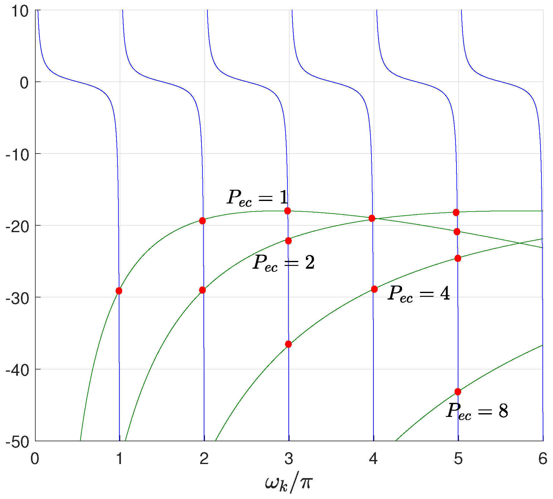
From Equations (19) and (20), it follows that numerical approximations are required to build the inyection term (Equation (5)). From Equation (13), for example, $l_1-l_0+1=-1$ and $\left|l_0\right|\gg 1$, Equation (20) becomes:

$${\left(tan\left({\omega }_k\right)\right)}^{-1}\approx -\left(\frac{1}{P_{ec}}{\omega }_k+{\left|l_0\right|}^2\frac{P_{ec}}{{\omega }_k}\right).$$

(21)

The right-hand side is a concave function with upper bound:

$$-\left(\frac{1}{P_{ec}}{\omega }_k+{\left|l_0\right|}^2\frac{P_{ec}}{{\omega }_k}\right)\le -2\left|l_0\right|,$$

(22)

and Equation (20) simply becomes:

$${\left(tan\left({\omega }_k\right)\right)}^{-1}\le -2\left|l_0\right|,$$

(23)

and using $\left|l_0\right|\gg 1$, we find:

$${\omega }_k\approx k\pi \mathrm{for}\mathrm{all}k\in \mathbb{N}.$$

(24)

In Figure 2, the left and right-hand sides of Equation (20) are plotted for $l_0=12$ and $l_1=10$, where the intersection points are the solutions of the equation, which verifies Equation (24).

Once the eigenfrequencies ${\omega }_k$ are fixed, Equation (19) becomes:

$$B_k=\frac{2k\pi A_k}{\left(1-2l_0\right)P_{ec}},$$

(25)

and for $\left|l_0\right|$ large enough, the first N terms may be neglected, this is:

$${\left.\left\{B_k\right\}\right|}_{k=1,\cdots ,N}\approx 0.$$

(26)

Therefore, the first N eigenfunctions are:

$${\varphi }_k\left(x\right)\approx A_k{exp}^{P_{ec}x/2}sin\left(k\pi x\right)k=\left\{1,\cdots ,N\right\}.$$

(27)

To satisfy the orthogonal condition depicted in the Appendix A (see Equation (A3)), $A_k=\sqrt{2}$ is selected for $k=\left\{1,\cdots ,N\right\}$, and the first N eigenfunctions become:

$${\varphi }_k\left(x\right)\approx \sqrt{2}{exp}^{P_{ec}x/2}sin\left(k\pi x\right)\mathrm{for}k=\left\{1,\cdots ,N\right\},$$

(28)

From where Equation (14) follows. In Figure 3, the first four eigenvalues for $l_0=12$ and $l_1=10$ are shown. Increasing $\left|l_0\right|$ will make Equation (28) a better approximation to the real eigenvalues.

From Equation (28), it is immediately obvious that the sensor should avoid any position $\xi \in \left(0,1\right)$ such that:

$$sin\left(\xi \pi x\right)=0\mathrm{for}k=\left\{1,\cdots ,N\right\},$$

(29)

and Equation (15) follows.

Now, noticing that the slowest N eigenfunctions are approximated by sine functions, the error decomposition $e\left(x,t\right)={\sum }_{k=1}^{\infty }{e}_k\left(t\right){\varphi }_k\left(x\right)$ may be written as:

$$e\left(x,t\right)=\sum _{k=1}^N{e}_k\left(t\right)A_{k}sin\left(k\pi x\right)+\sum _{k=N+1}^{\infty }{e}_k\left(t\right){\varphi }_k\left(x\right).$$

(30)

Therefore, at the boundaries:

$${\left.e\left(x,t\right)\right|}_{x=\left\{0,1\right\}}=\sum _{k=N+1}^{\infty }{e}_k\left(t\right){\varphi }_k\left(x\right),$$

(31)

the error depends only of fastest modes ${\left.\left\{{\varphi }_k\left(x\right)\right\}\right|}_{k=\left\{N+1,\cdots \right\}}$ that converges rapidly to zero.

Remark 2.

If the values of $B_k$ for $k=\left\{1,2,...,N\right\}$ are not negligible, this may occur for small Peclet numbers or $l_0$ close to $\frac{1}{2}$ (see Equation (19)); then, a peaking phenomenon may arise. This is exemplified in the numerical simulation section.

Remark 3.

Equation (13), say $l_1=l_0-2$ is an algebraic condition, not the only one, proposed to preserve the right-hand side of Equation (20) as a concave function, keeping valid the approximation ${\omega }_k\approx k\pi$.

The precise sensor position is something that should be discussed more carefully; however, noticing that the sensor position $\xi$ should be selected to increase the effect of the correction mechanism, given by the product $l_{\xi }\left(x\right)e\left(\xi ,t\right)$ in Equation (4), the sensor position can be proposed to satisfy the relation:

$$\xi =\left\{y:\sum _{j=1}^N\left|{\varphi }_j\left(y\right)\right|=\underset{x\in \left(0,1\right)}{max}\sum _{j=1}^N\left|{\varphi }_j\left(x\right)\right|\right\}.$$

(32)

4. Numerical Simulation

In this section, a tubular reactor with a non-monotonic Langmuir–Hinshelwood type kinematics is considered [2,3], where the reaction rate is given by:

$$r\left(c\left(x,t\right)\right)=\frac{c\left(x,t\right)}{{\left(1+\sigma c\left(x,t\right)\right)}^2},$$

(33)

where the constant coefficient $\sigma$ denotes some inhibition parameter. Simulation studies were carried out, considering a diffusion dominated behaviour corresponding to $\left(P_{ec},\sigma ,D_a\right)=\left(6,3,4\right)$, and an inflow as the sum of a nominal and a perturbation term:

$$c_{in}\left(t\right)=\underset{\mathrm{nominal}}{\underbrace{0.3}}+\underset{\mathrm{perturbation}}{\underbrace{0.1\left(\sum _{m=0}^{5}cos\left(6m\pi t\right)\right)}}.$$

(34)

Figure 4 shows the error surface when no correction mechanism is applied, this is, $l_0=l_1=l_{\xi }=0$. The behaviour at $x=0$ is due to the inflow perturbations.

By setting $\left\{l_0,l_1\right\}=\left\{102,100\right\}$, the error in the boundaries can be brought to values close to zero rapidly (see Figure 5); even the effect of the inflow perturbations is reduced. Note that without the modal injection mechanism $l_{\xi }\left(x\right)$, at $t=0.6$ (s), the spatial behaviour of the error resembles the behaviour of the first and slowest eigenfunction ${\varphi }_1\left(x\right)=\sqrt{2}{exp}^{P_{ec}x/2}sin\left(\pi x\right)$.

Now, it is straightforward to verify condition (iii) of Theorem 1; this is, the eigenvalues form the decreasing series:

$$\begin{array}{cccc}{\lambda }_1=-3.15,& {\lambda }_2=-8.08,& {\lambda }_3=-16.30,& \cdots \end{array}$$

(35)

and Equation (11) is fulfilled for $N=1$:

$$-2{\lambda }_{N+1}>\frac{{\left(2D_a-\left[s_u+s_l\right]\right)}^2}{4}-s_u{s}_l+2\mathsf{\Lambda }=12.41+2\mathsf{\Lambda },$$

(36)

and any $\mathsf{\Lambda }\in \left(0,1.87\right)$. It is proposed the modal correction mechanism:

$$l_{\xi }\left(x\right)=l_{\xi ,1}{\varphi }_1\left(x\right)=l_{\xi ,1}\sqrt{2}{exp}^{P_{ec}x/2}sin\left(\pi x\right),$$

(37)

that will affect the slowest eigenfunction, allowing a better convergence of the error surface to zero. Using Equation (32) to fix the sensor position to $\xi =0.74$, and by setting $l_{\xi ,1}=2.87$, condition (iv) of the Theorem 1 is fulfilled:

$${\lambda }_1-l_{\xi ,1}\varphi \left(\xi \right)=-30<{\lambda }_2.$$

(38)

In Figure 6, the error surface with the the boundary feedback and the correction mechanism is shown. The effect of the modal injection mechanism is immediate.

Figure 7 shows the error norm $E\left(t\right)$ for all different feedback conditions:

(a)

No feedback;

(b)

only boundary feedback;

(c)

only modal correction mechanism;

(d)

both boundary and modal correction mechanism.

The combination of a modal injection mechanism with boundary feedback increases the convergence rate without compromising stability. To improve the observer convergence, more modes can be added to the modal correction mechanism; for example, consider the modal correction mechanism:

$$l_{\xi }\left(x\right)=\sum _{k=1}^3{l_{\xi }}_{,k}{\mathsf{\Phi }}_k\left(x\right)=\sqrt{2}{exp}^{P_{ec}x/2}\sum _{k=1}^3{l_{\xi }}_{,k}sin\left(k\pi x\right).$$

(39)

It is immediate to verify that setting:

$$\begin{array}{ccccc}{l}_{\xi ,1}=12.6,& & l_{\xi ,2}=6.2,& & l_{\xi ,3}=0.3,\end{array}$$

(40)

then:

$$max\left\{\mathrm{eig}\left(\left[\begin{array}{ccc}-3.15& 0& 0\\ 0& -8.08& 0\\ 0& 0& -16.30\end{array}\right]-\left[\begin{array}{c}{l}_{\xi ,1}\\ l_{\xi ,2}\\ l_{\xi ,3}\end{array}\right]\left[\begin{array}{ccc}{\varphi }_1\left(\xi \right)& {\varphi }_2\left(\xi \right)& {\varphi }_3\left(\xi \right)\end{array}\right]\right)\right\}=-20<{\lambda }_3,$$

(41)

and the convergence rate of the three slowest modes is increased. In Figure 8, the corresponding error surface is shown. Comparing Figure 6 and Figure 8, the effect of adding more modes in the modal correction mechanism is immediate.

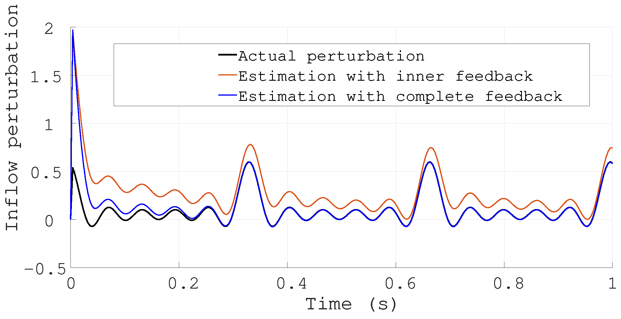
Now, using the fact that the error in the boundaries is close to zero, this is:

$$\begin{array}{ccc}{\left.e\left(x,t\right)\right|}_{x=0}\approx 0& \Rightarrow & \widehat{c}\left(0,t\right)\approx c\left(0,t\right)\end{array},$$

(42)

simple numeric manipulations will allow the estimation of the inflow perturbation. From the boundary conditions:

$$\frac{1}{P_{ec}}\frac{\partial c\left(0,t\right)}{\partial x}=c\left(0,t\right)-\left\{c_{\mathrm{in}}\left(t\right)+{\theta }_{\mathrm{per}}\left(t\right)\right\},$$

(43)

and the corresponding discrete approximation:

$$\frac{1}{P_{ec}\Delta x}\left(c\left(\Delta x,t\right)-c\left(0,t\right)\right)=c\left(0,t\right)-\left\{c_{\mathrm{in}}\left(t\right)+{\theta }_{\mathrm{per}}\left(t\right)\right\},$$

(44)

a non-rigorous estimation of the perturbation is obtained by replacing the actual concentration with the estimated concentration, this is, $c\left(\Delta x,t\right)\to \widehat{c}\left(\Delta x,t\right)$, and solving for ${\theta }_{\mathrm{per}}$ as:

$${\theta }_{\mathrm{per}}\left(t\right)\approx \frac{1}{P_{ec}\Delta x}\left(\left(1+P_{ec}\Delta x\right)c\left(0,t\right)-\widehat{c}\left(\Delta x,t\right)\right)-c_{\mathrm{in}}\left(t\right).$$

(45)

The estimation of the inflow perturbation is shown in Figure 9.

Finally, and for completeness, an example is presented of the peaking phenomenon that commonly occurs when high gains are implemented.

Peaking Phenomenon

Consider a tubular reactor with a small Peclet number, for example, $\left(P_{ec},\sigma ,D_a\right)=\left(2,3,4\right)$, and the boundary gains $\left(l_0,l_1\right)=\left(12,10\right)$. The corresponding error surface is depicted in Figure 10, where a peak in the spatial boundary appears. Contrary to what is thought, this peak is reduced when the boundary gains are increased, making this peaking phenomenon something that should be more carefully analysed, especially when the observer data will be used for feedback control [20].

5. Conclusions

In this work, we extend some results of the non-linear dissipative observer to show that correctly chosen boundary gains allow a simple tuning of the observer and its parameters, improving the observer convergence, and allowing the estimation of the inflow perturbations. Numerical validation of the presented algorithm shows the validity of the proposed approach.

References

- Lapidus, L.; Amundson, N. Chemical Reactor Theory; Printice-Hall: Upper Saddle River, NJ, USA, 1977. [Google Scholar]
- Carberry, J.J. Chemical and Catalytic Reaction Engineering; Courier Corporation: Chelmsford, MA, USA, 2001. [Google Scholar]
- Elnashaie, S.S.; Abashar, M.E. The implication of non-monotonic kinetics on the design of catalytic reactors. Chem. Eng. Sci. 1990, 45, 2964–2967. [Google Scholar] [CrossRef]
- Bailey, J.E.; Ollis, D.F. Biochemical engineering fundamentals. Chem. Eng. Educ. 1976, 10, 162–165. [Google Scholar]
- Curtain, R.F.; Demetriou, M.A.; Ito, K. Adaptive compensators for perturbed positive real infinite- dimensional systems. Int. J. Appl. Math. Comput. Sci. 2003, 13, 441–452. [Google Scholar]
- Mercorelli, P. An adaptive and optimized switching observer for sensorless control of an electromagnetic valve actuator in camless internal combustion engines. Asian J. Control 2014, 16, 959–973. [Google Scholar] [CrossRef]
- Mercorelli, P. A motion-sensorless control for intake valves in combustion engines. IEEE Trans. Ind. Electron. 2017, 64, 3402–3412. [Google Scholar] [CrossRef]
- Krstic, M.; Smyshlyaev, A. Boundary Control of PDEs: A Course on Backstepping Designs; Siam: Philadelphia, PA, USA, 2008; Volume 16. [Google Scholar]
- Orlov, Y.V. Discontinuous Systems: Lyapunov Analysis and Robust Synthesis under Uncertainty Conditions; Springer Science & Business Media: Berlin, Germany, 2008. [Google Scholar]
- Schaum, A.; Alvarez, J.; Meurer, T.; Moreno, J. State-estimation for a class of tubular reactors using a pointwise innovation scheme. J. Process Control 2017, 60, 104–114. [Google Scholar] [CrossRef]
- Chen, L.; Mercorelli, P.; Liu, S. A Kalman estimator for detecting repetitive disturbances. In Proceedings of the 2005 IEEE American Control Conference, Portland, OR, USA, 8–10 June 2005; pp. 1631–1636. [Google Scholar]
- Kharkovskaia, T.; Efimov, D.; Fridman, E.; Polyakov, A.; Richard, J.P. On design of interval observers for parabolic PDEs. IFAC-PapersOnLine 2017, 50, 4045–4050. [Google Scholar] [CrossRef]
- Schaum, A.; Moreno, J.A.; Alvarez, J. Spectral dissipativity observer for a class of tubular reactors. In Proceedings of the 47th IEEE Conference on Decision and Control, CDC 2008, Cancun, Mexico, 9–11 December 2008; pp. 5656–5661. [Google Scholar]
- Pourkargar, D.B.; Armaou, A. Design of APOD-based switching dynamic observers and output feedback control for a class of nonlinear distributed parameter systems. Chem. Eng. Sci. 2015, 136, 62–75. [Google Scholar] [CrossRef] [Green Version]
- Pourkargar, D.B.; Armaou, A. Dynamic shaping of transport–reaction processes with a combined sliding mode controller and Luenberger-type dynamic observer design. Chem. Eng. Sci. 2015, 138, 673–684. [Google Scholar] [CrossRef] [Green Version]
- Schaum, A.; Moreno, J.; Meurer, T. Dissipativity-based observer design for a class of coupled 1-D semi-linear parabolic PDE systems. IFAC-PapersOnLine 2016, 49, 98–103. [Google Scholar] [CrossRef]
- Schaum, A.; Moreno, J.A.; Díaz-Salgado, J.; Alvarez, J. Dissipativity-based observer and feedback control design for a class of chemical reactors. J. Process Control 2008, 18, 896–905. [Google Scholar] [CrossRef]
- Schaum, A. On the Design of Nonlinear Dissipative Observers for Agitated and Tubular Reactors. Ph.D. Thesis, Instituto de Ingeniería, Universidad Nacional Autónoma de México, Mexico City, Mexico, 2009. [Google Scholar]
- Delattre, C.; Dochain, D.; Winkin, J. Sturm-Liouville systems are Riesz-spectral systems. Int. J. Appl. Math. Comput. Sci. 2003, 13, 481–484. [Google Scholar]
- Sussmann, H.; Kokotovic, P. The peaking phenomenon and the global stabilization of nonlinear systems. IEEE Trans. Autom. Control 1991, 36, 424–440. [Google Scholar] [CrossRef]
- Dettman, J.W. Mathematical Methods in Physics and Engineering; Courier Corporation: Chelmsford, MA, USA, 2013. [Google Scholar]
- Jeffreys, H.; Jeffreys, B. Methods of Mathematical Physics; Cambridge University Press: Cambridge, UK, 1999. [Google Scholar]
Figure 1.
Simplified model of a tubular reactor.
Figure 2.
Numerical approximation for Equation(20).
Figure 3.
First four eigenvalues .
Figure 4.
Error surface without boundary feedback.
Figure 5.
Error surface with only boundary feedback.
Figure 6.
Error surface with boundary and the first mode feedback.
Figure 7.
Error comparison.
Figure 8.
Error surface with boundary and three modal correction mechanism.
Figure 9.
Perturbation estimation in the concentration input.
Figure 10.
Peaking phenomena is the error surface.
© 2018 by the authors. Licensee MDPI, Basel, Switzerland. This article is an open access article distributed under the terms and conditions of the Creative Commons Attribution (CC BY) license (http://creativecommons.org/licenses/by/4.0/).
Share and Cite
MDPI and ACS Style
Gutierrez-Carmona, I.; Moreno, J.A.; Abundis-Fong, H.F. On the Boundary Conditions in a Non-Linear Dissipative Observer for Tubular Reactors. Processes 2019, 7, 8. https://doi.org/10.3390/pr7010008
AMA Style
Gutierrez-Carmona I, Moreno JA, Abundis-Fong HF. On the Boundary Conditions in a Non-Linear Dissipative Observer for Tubular Reactors. Processes. 2019; 7(1):8. https://doi.org/10.3390/pr7010008
Chicago/Turabian StyleGutierrez-Carmona, Irandi, Jaime A. Moreno, and H.F. Abundis-Fong. 2019. "On the Boundary Conditions in a Non-Linear Dissipative Observer for Tubular Reactors" Processes 7, no. 1: 8. https://doi.org/10.3390/pr7010008
Note that from the first issue of 2016, this journal uses article numbers instead of page numbers. See further details here.