Layout Optimization Process to Minimize the Cost of Energy of an Offshore Floating Hybrid Wind–Wave Farm

Abstract

Offshore floating hybrid wind and wave energy is a young technology yet to be scaled up. A way to reduce the total costs of the energy production process in order to ensure competitiveness in the sustainable energy market is to maximize the farm’s efficiency. To do so, an energy generation and costs calculation model was developed with the objective of minimizing the technology’s Levelized Cost of Energy (LCOE) of the P80 hybrid wind-wave concept, designed by the company Floating Power Plant A/S. A Particle Swarm Optimization (PSO) algorithm was then implemented on top of other technical and decision-making processes, taking as decision variables the layout, the offshore substation position, and the export cable choice. The process was applied off the west coast of Ireland in a site of interest for the company, and after a quantitative and qualitative optimization process, a minimized LCOE was obtained. It was then found that lower costs of ~73% can be reached in the short-term, and the room for improvement in the structure’s design and materials was highlighted, with an LCOE reduction potential of up to 32%. The model serves usefully as a preliminary analysis. However, the uncertainty estimate of 11% indicates that further site-specific studies and measurements are essential.

1. Introduction

One of the main conditioning issues of the planet’s climate since the industrial revolution is global warming, a consequence of greenhouse gases in the atmosphere. More than 97% of the scientific community agree on the fact that human emissions are the main reason of this phenomenon [1]. Consequently, since the late 1990s, several efforts have been launched at the international level. Among other targets, middle-term national green new deals point at a transition to a full sustainable energy generation system as it is one of the main sources of these greenhouse gas emissions, representing around 25% of them according to the Intergovernmental Panel on Climate Change (IPCC) [2].

Wind energy plays a crucial role in this transition, as it currently supplies 14% of Europe’s and 6% of the world’s total electricity demand [3] with a total installed capacity of 597 GW by the end of 2018 [4], of which 23 GW corresponds to offshore farms worldwide [5]. This newly exploitable offshore resource presents significant advantages with respect to that available onshore as it is both more constant and powerful: two very valuable characteristics for the energy market. These features combined with the lower spatial constraints in the sea have allowed the manufacturers to develop bigger turbines that currently reach capacities of up to 12 MW [6].

State-of-the-art floating concepts allow the access to an even more ideal wind resource in areas where the installation of bottom-fixed turbines is unfeasible today. An additional step in the latest floating technologies are the hybrid concepts that combine different sources of energy, thus allowing the efficient exploitation of more than one energy source. One of the most developed concepts is the hybrid wind and wave technology, combining Wind Turbine Generators (WTG) and Wave Energy Converters (WEC), and leading to an increase of the energy yield, a smoother and more reliable output power, and the opening of the Operation and Maintenance (O&M) window thanks to the waves shadow effect, thus reducing the project’s costs [7,8]. This leads to the device object of this study: the P80, a semi-submersible hybrid wind and wave concept designed by Floating Power Plant A/S (FPP) in Denmark [9].

One of the ways to ensure the competitiveness of state-of-the-art technologies is maximizing the usage efficiency of the existing designs, which is the target of this study. A P80 farm layout optimization model integrated by technical, mathematical, and decision processes was developed with the objective of minimizing the total lifetime energy generation costs of a project with the P80. Given the nature of this type of optimization problem, which presents spatial constraints, discrete values, and convexity, the optimization needs to be carried out through meta-heuristic algorithms [10], extensively used in the wind energy field [11,12,13,14]. The optimization process is then carried out by means of a Particle Swarm Optimization (PSO) algorithm, based in bird flocking, fish schooling, and swarming theory [15]. The objective function subject to be minimized in the model is the Levelized Cost of Energy (LCOE), as it represents the average generation cost of a unit of energy throughout the lifetime of a project, thus being a powerful indicator that allows investors to compare the variation of costs with time, among different arrangements and technologies [16].

Once developed, the tool was applied to optimize a potential project in a specific area of interest off the west coast of the Republic of Ireland, together with analyses of other qualitative particularities of the region. An optimal minimization of the LCOE was reached where significant costs reductions were found. To maintain the company’s confidentiality, the LCOE figures obtained are expressed as indexed values throughout the report.

The work detailed in this paper is the result of a combination of engineering processes in terms of wind and waves energy exploitation, a cost modeling process with the subsequent analysis of the project’s energy yield and business case drivers, the optimization process of the farm layout (among other parameters), and a decision-making process with regard to the development of a farm project, based on engineering and project management foundations.

This paper is structured as follows. In Section 2, the relevant details regarding the model’s construction are explained. After a qualitative study, the application of the model in a geographical area of relevance for FPP located off the west coast of the Republic of Ireland is presented: different sites within the area are considered and an ideal final site and layout are chosen after a description of the optimization process that was followed; this constitutes Section 3. Finally, a discussion about the results is performed in Section 4.

2. Materials and Methods

In this section, an overview of the model used in the optimization process is first presented to put the optimization process in context. After introducing the model components, the most relevant equations involved in the optimization process, focus of this study, and the constraints associated to it are presented. Last, the used optimization algorithm is concisely explained.

As shown in Figure 1, the tool is composed of four main modules: the wind and waves power generation models, the costs calculation model and finally, the overall optimization algorithm that modifies the decision variables, thus improving the output of the model in an iterative way. The waves and wind power production modules aim at simulating the physical and technical phenomena that result in a certain Annual Energy Production (AEP), including the interaction between platforms (wind wakes and waves shadows). This is the source of most of the nonlinearities of the model. Their detailed description can be found in [17] together with an outline of FPP’s P80 technology.

The tool presented in the diagram of Figure 1 consists of a lifetime energy generation and costs calculation of an offshore hybrid farm project. The farm is composed of several P80 platforms that are connected to an offshore floating electrical substation through inter-array cables; from the offshore substation, an export cable transmits the electricity produced in the farm to an inland electrical substation which is connected to the grid; furthermore, a harbor is used to carry out the marine operations in the farm.

2.1. The Costs Model

The costs model is a series of economical calculations, mostly linear, that use these AEP results as inputs to find the costs of the project in relation to the energy production by means of the LCOE indicator. The costs model includes the costs due to the capital expenses (CAPEX); the costs derived from the operational expenditures (OPEX); and those associated to the energy losses due to the generators’ downtime periods and transmission of the electricity. The inputs to the costs model are the gross AEP from the wind and the waves after the wakes and shadow losses, the values related to the site characterization (bathymetry and coordinates, and the inland substation, harbor, and shore positions), and more than 140 costs related figures. The output is the $LCOE$, introduced below.

2.1.1. Levelized Cost of Energy (LCOE)

The $LCOE$, expressed in $€/MWh$, indicates the average cost of the energy produced throughout the lifetime of a project, and therefore the minimum average price at which the energy must be sold to make the project feasible [16]. Unlike other simpler indicators, the $LCOE$ takes into account the time value of money, as it weights the annual expenses $T{C}_t$ in each year t by means of a discount rate r, which is determined by the investors according to the inflation and the estimated risk of the project. It is arguably the most useful indicator for seeking financing as it is ideal to compare the costs of different technologies [18]. The $LCOE$ is calculated in the model as follows,

$$LCOE=\frac{{\sum }_{t=0}^{LT}\frac{T{C}_t}{{(1+r)}^t}}{{\sum }_{i=0}^{LT}\frac{q_t}{{(1+r)}^t}}$$

(1)

where $q_t$ represents the yearly energy production in period t (obtained in the wind and waves models), and $LT$ the lifetime of the project. The annual expenses included in $T{C}_t$ are presented below. As stated above, in this paper the LCOE values are expressed as dimensionless indexed numbers where the relative change is well represented.

2.1.2. Capital Expenditures (CAPEX)

The capital expenditures of a project involve all the investment, administrative, acquisition and installation related costs before and along its lifetime. They are calculated as follows,

$$CAPE{X}_i=C_{PM,i}+C_{WTG,i}+C_{P80,i}+C_{Moor,i}+C_{EI,i}+C_{Inst,i}+C_{Decom,i}$$

(2)

The categories considered in the model are design and project management expenses ($C_{PM}$), wind turbine acquisition cost ($C_{WTG}$), P80 costs ($C_{P80}$), mooring costs ($C_{Moor}$), costs associated to the electrical infrastructure ($C_{EI}$), installation costs ($C_{Inst}$), and decommissioning costs ($C_{Decom}$); all of them expressed in €.

• The “design and project management” costs are applied in year zero and they are divided into concession ($C{}_{concession}$) and design ($C{}_{design}$) costs:

$$C_{PM}=C_{concession}+C_{design}$$

(3)

$$C_{concession}=C_{con.,cap}·Ca{p}_{Tot}$$

(4)

$$C_{design}=Margin·\left(C_{P80}+C_{transp}+C_{ass}\right)$$

(5)

being

$C_{con.,cap}[€/MW]$	estimation of concession costs per capacity unit.
$Ca{p}_{Tot}\left[MW\right]$	total capacity of the farm.
$Margin[\%]$	FPP’s margin as a percentage of investment costs.
$C_{P80}[€]$	acquisition cost of the P80.
$C_{transp}[€]$	cost of components’ transportation to assembly site.
$C_{ass}[€]$	P80 assembly costs.

• The acquisition cost of the wind turbines, one of the main cost components of a wind farm project, is calculated as a linear function of the wind turbine capacity:

$$C_{WTG}=C_{WTcap.}·Ca{p}_{WT}$$

(6)

where

$Ca{p}_{WT}\left[MW\right]$	is the total capacity of the farm.
$C_{WTcap.}[€/MW]$	is the considered cost per capacity.

• The acquisition costs of the P80 platform include the costs associated to the platform’s structure and the waves energy converter (absorbers and power take-off system). They are calculated as follows,

$$C_{P80}=C_{plat}·n_{plat}+C_{site}$$

(7)

where

$C_{plat}[€/P80]$	is the cost of a P80 platform.
$n_{plat}$	is the number of platforms.
$C_{site}[€]$	are costs associated to condition monitoring and the SCADA systems.

• The mooring costs ($C_{Moor}$, in €) are divided into the anchor acquisition costs, which include the six anchor kits needed in each P80 unit, and the mooring line costs, which are considered to increase linearly with depth:

$$C_{Moor}={\displaystyle \sum _{i=1}^{n_{plat}}}{C}_{anch.}+C_{lines}·\frac{l}{d}·d_i$$

(8)

being

$C_{anch.}[€/P80]$	fixed cost of a platform’s mooring system (anchors, buoyancy elements, etc.).
$C_{lines}[€/m]$	length dependent cost of the mooring lines.
$l/d$	linear rate of mooring lines length per seafloor depth.
$d_i\left[m\right]$	depth under platform i.

• The investment costs associated to the electrical infrastructure are composed of those associated to the inter-array cables ($C_{MV}$), the export high voltage cable ($C_{HV}$), the offshore substation ($C_{sub.}$), and some additional costs associated to other devices ($C_{el.other}$):

$$C_{EI}=C_{MV}+C_{HV}+C_{sub.}+C_{el.other}$$

(9)

The cables costs are modeled as a linear function of their length, the additional costs depend on the number of platforms, and the substation’s costs are calculated as follows [19]:

$$C_{sub.}=\mathrm{539,000}·Ca{p}_{Tot}^{0.687}$$

(10)

• The installation costs are those expenses associated to both the human workforce and the technology used in the transportation, assembly, connection, and testing of all the infrastructure involved in the construction of the farm up to its commissioning:

$$C_{Inst.}=C_{transp.}+C_{ass.}+C_{inst.moor.}+C_{inst.elec.}+C_{inst.P80}+C_{connec.}$$

(11)

where the presented elements describe the various installation processes involved at the beginning of the project. They correspond to the following.

$C_{transp.}[€]$	is the cost of transportation of the components to the assembly site.
$C_{ass.}[€]$	assembly costs.
$C_{inst.moor.}[€]$	mooring installation costs.
$C_{inst.elec.}[€]$	costs of installation of the electrical infrastructure.
$C_{inst.P80}[€]$	costs of on-site platforms installation.
$C_{connec.}[€]$	commissioning or connection costs.

Most of these costs, not detailed here for the sake of brevity, but specified in [17], are fixed or of linear nature depending on variables such as the number of elements (e.g., platforms), length of cable used, cable laying speed, cruise speed of cable lying, and so on, multiplied by the unitary cost of those items.

• Finally, the decommissioning costs are calculated. They are applied in the last year of the project’s lifetime. The costs due to the removal of all the installed elements may be expressed as

$$C_{Decom}=C_{d.grid}+C_{d.P80}+C_{d.moor.}+C_{d.other}$$

(12)

representing the various decommissioning categories, namely, costs related to

$C_{d.grid}[€]$	the electrical infrastructure.
$C_{d.P80}[€]$	the platforms.
$C_{d.moor.}[€]$	the mooring system.
$C_{d.other}[€]$	the paperwork involved in the process.

Once again, most of these costs are of linear nature.

2.1.3. Operational Expenditures (OPEX)

The Operational Expenditures include the costs associated to all types of maintenance and any other operation along the lifetime of a project (e.g.,: inspections, checks, testing, cleaning, painting, replacement of components, etc.), being often divided into planned and unplanned or unscheduled O&M [20]. These maintenance operations have an associated energy generation downtime, as they often involve a failure or require shutting down the generators. The generation downtime is thus modeled together with the O&M costs as part of the OPEX.

As done when modeling the CAPEX, and more relevantly in this case, due to its distribution along the years, the annual costs associated to the OPEX are calculated individually every year, so they can be discounted in the LCOE calculation as explained above. Thus, for each year, i, in the project’s lifetime, the maintenance operations ($O\&M_i$, in €) and their associated downtime ($D{T}_i$, in hours) are calculated as follows.

$$O\&M_i=O\&M_{planned,i}+O\&M_{unplanned,i}$$

(13)

$$D{T}_i=D{T}_{planned,i}+D{T}_{unplanned,i}$$

(14)

• Planned O&M and Downtime: there are different types of planned O&M operations: yearly, intermediate, and major operations; each of which has an associated frequency, cost and downtime period. Depending on the planned operations in each year i, the associated costs and downtime periods are expressed as follows,

$$O\&M_{planned,i}=C_{O\&Msite}+n_{plat}·C_{O\&MP80,i}$$

(15)

$$D{T}_{planned,i}=t_{O\&M,i}$$

(16)

where,

$C_{O\&Msite}[€/year]$	the fixed yearly O&M cost: port charges, fixed costs of vessels, etc.
$C_{O\&MP80,i}[€/P80/year]$	the O&M cost per platform in year i.
$t_{O\&M,i}[h/year]$	hours of planned downtime in year i.

• Unplanned O&M and Downtime. In the case of the operations due to unexpected or sudden breakdowns, the costs and their associated downtimes are implemented by sorting the failures into five different severity levels: remote reset, minor fault/ inspection, medium fault (module replacement), large fault (offshore repair), and major fault (harbor repair). Each one of these categories presents a certain occurrence probability that is translated in the model as a number of incidents per year. The yearly unplanned O&M costs and downtime are thus implemented in the model as shown below,

$$O\&M_{unplanned}={\displaystyle \sum _{i=1}^5}\left\{n_{plat}·f_{fail,i}·\left[C_{fixed,i}+C_{h,i}·\left(t_{rep,i}+\frac{d_{harb}}{s_{go,i}}+\frac{d_{harb}}{s_{ret.,i}}\right)\right]\right\}$$

(17)

$$D{T}_{unplanned}={\displaystyle \sum _{i=1}^5}\left[f_{fail,i}·\left(t_{rep,i}+\frac{d_{harb}}{s_{go,i}}\right)\right]$$

(18)

where

$f_{fail,i}$	estimated number of failures per year for failure type i.
$C_{fixed,i}[€/P80]$	fixed repair cost per failure for failure type i (mobilization costs, etc.).
$C_{h,i}[€/h/P80]$	time dependent cost for failure type i (it includes personnel, vessel costs, etc.).
$t_{rep,i}\left[h\right]$	repair time for failure type i.
$d_{harb}\left[km\right]$	average distance to harbor.
$s_{go,i}[km/h]$	going speed of the vessel used in failure type i.
$s_{ret.,i}[km/h]$	return speed of the vessel used in failure type i.

2.2. Optimization

Given the wide range of variables involved in the model, the nature of many of the parameters (some of which are discrete and cannot be easily described by explicit functions and/or involve specific processes for their calculation), the spatial constraints, and the lack of convexity (the presence of several minima), it is not feasible to carry out a classical analytical or gradient-based optimization [11,12]. For this reason, it is necessary to use meta-heuristic methods instead, for example evolutionary algorithms. They are calculation methods that take metaphorical inspiration on certain processes that occur in nature [10]. They work by improving the obtained results in an iterative way, modifying the decision variables in each iteration according to the algorithm’s working principle or logic.

The Genetic Algorithm (GA) and the Particle Swarm Optimization (PSO) are among the most used methods. The former, extensively used in the wind energy field [11,13,14], emulates the principles of evolution theory by combining and mutating offspring solutions that give birth to new ones. With regard to the PSO, it is based on bird flocking, fish schooling, or swarming theory, also having strong ties with the GA [15]. Additionally, in the optimization field, and taking into consideration the description of the problem, both single and multi-objective algorithms may be used. As an example of a multi-objective algorithm, the Agent Swarm Optimization (ASO), originated in the water supply field, shall be mentioned. ASO integrates behaviors of the two described algorithms, among others, preventing it from terminating in local minima, thus increasing the efficiency and, as a result, the total time devoted to solve the problem [21,22].

In this work, as a first approximation, it was used the classical PSO in a single objective optimization setting. The algorithm was set up to obtain the minimum LCOE in any site with its specific inputs. The coding was carried out in MATLAB with inputs provided by Excel data sheets following three objectives: first, minimizing as much as possible the many uncertainties involved in this complex calculation, naturally still assuming some limitations; second, reducing its running time, especially for the sake of the optimization process; and, third, developing it in a user-friendly manner.

2.2.1. Particle Swarm Optimization

The PSO is primarily based on the movement of the different individuals (in this case known as particles, each of which represents a set of decision variables) with respect to the rest of the members (population) of the swarm [15]. The new variables used in each iteration shift from their predecessors according to three different components [23]: the current (time k) position of a particle i, namely, $x_i\left(k\right)$; the best position ever achieved by the particle, $x_i^{pbest}$; and the global best position, $x^{nbest}$, achieved by any of the particles in the swarm (or neighborhood). The current position of the particle is updated through addition of its velocity, calculated as

$$v_i(k+1)=\omega ·v_i\left(k\right)+c_1·r_1·\left(x_i^{pbest}\left(k\right)-x_i\left(k\right)\right)+c_2·r_2·\left(x_i^{nbest}\left(k\right)-x_i\left(k\right)\right)$$

(19)

In this expression, $\omega$ is the inertia parameter, $c_1$ the cognitive/own-best position/self-adjustment weight, and $c_2$ the neighborhood/social/group adjustment weight, the factors that influence the particle’s motion; $r_1$ and $r_2$ are random numbers within $[0,1]$ to represent nature’s inexact condition.

Four main parties are involved in the way the optimization process is built: the objective function (minimization of the LCOE, already described in Section 2.1.1), the decision variables (subject of change to improve the result), the decision variables’ associated constraints, and the penalties (increase of the objective value due to the infringement of the constraints).

2.2.2. Decision Variables

Among the wide range of parameters that could be subject of change to minimize the LCOE, in the last version of the optimization algorithm eight parameters, divided in three groups, were chosen as decision variables, as described below.

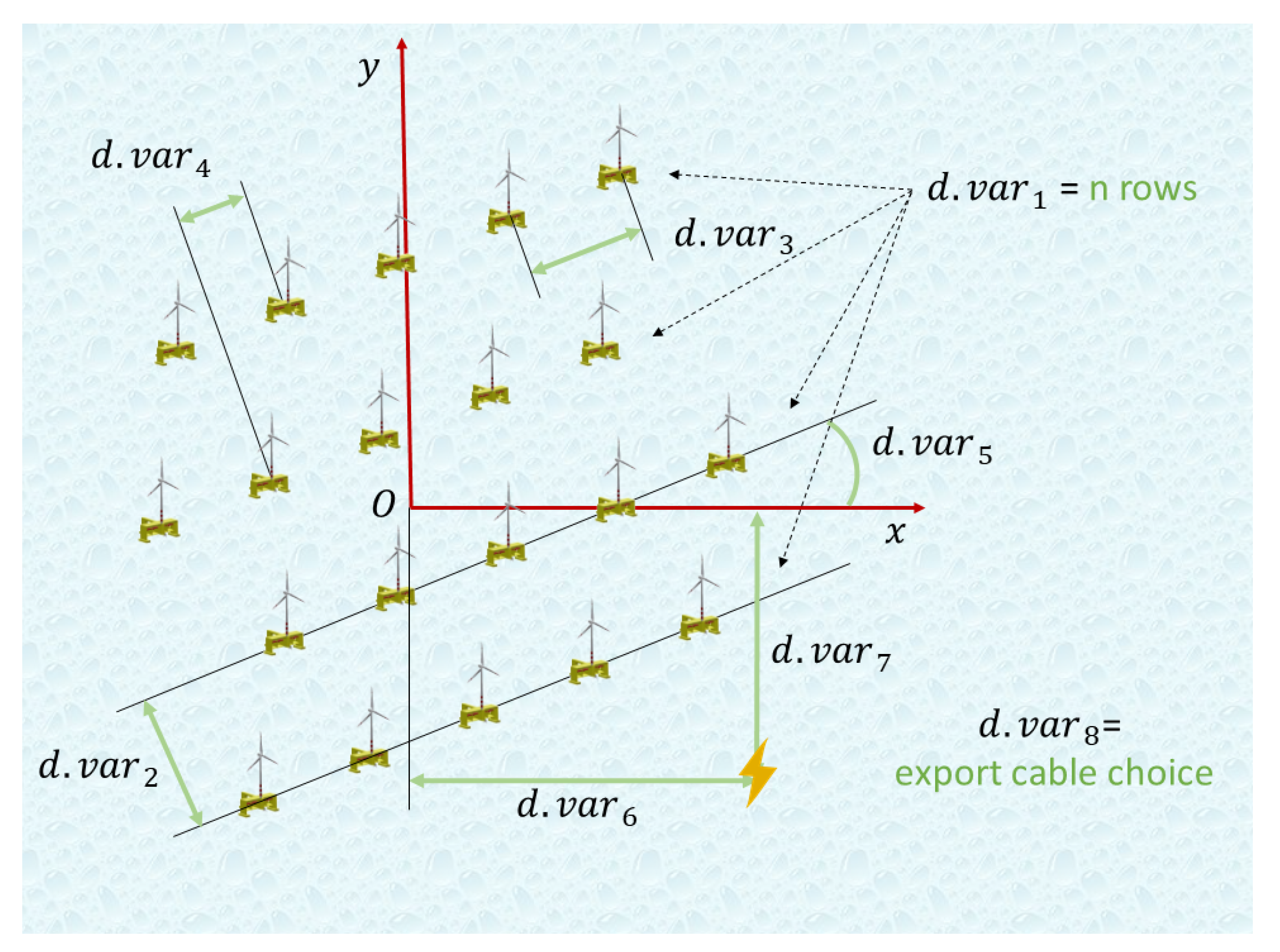
• First, the decision variables associated to the positions of the platforms: arguably, the most relevant decision variables of the model. With a set number of platforms in the farm, different ways of arranging the turbines were considered. At first, the platforms were allowed to be located independently within the limited site’s area. However, rather messy and unorganized arrangements were obtained, and this option was soon discarded due to consequent negative visual impact and the operational difficulties that this may involve (e.g., definition of boat routes and safe access areas). Moreover, this arrangement method involved having 2 decision variables per platform (x and y coordinates), which increased the computational time and decreased the efficiency of the algorithm significantly. To solve these issues, the platforms were finally arranged in rows and it was resolved that a total of five decision variables were necessary to define completely the positions of all the platforms: these are the number of rows ($d.va{r}_1$); the separation between rows ($d.va{r}_2$); the separation between platforms in each row ($d.va{r}_3$); the row offset ($d.va{r}_4$), i.e., the relative positional shift along the rows’ direction of consecutive rows; and the orientation angle of the rows ($d.va{r}_5$). As it can be seen in Figure 2, the platforms are located around the site’s center coordinates, so the rows are distributed equally to each side. These input parameters or decision variables are then converted into the platforms coordinates inside the function: first, the number of platforms and rows is read, and therefore the rows are created with their specified spacing ($d.va{r}_2$ and $d.va{r}_3$); then, the uneven extra platforms are successively added from the last row towards the first one; finally, the orientation angle is applied by multiplying each platform’s coordinates by a a two-dimensional rotation matrix ($R_{\theta }$).
• The second group of decision variables ($d.va{r}_6$ and $d.va{r}_7$) are the coordinates of the offshore substation, specified as x and y distances with respect to the center of the site O.
• Finally, the last decision variable ($d.va{r}_8$) is the farm’s export cable choice among the available ones, which has an impact in the costs and transmission losses as the chosen cable has its own specifications.

A number of other parameters that a priori seemed subject of becoming decision variables were eventually disregarded as such due to various reasons. These parameters are the following.

• Harbor and inland substation choice among the available ones in the area: even though the LCOE output is definitely influenced by this decision, there are many external factors that condition it as this choice highly depends on the state legislation and planning; it also depends on particular characteristics of both the harbour and substation: their size, availability, grid strength, and so on. Therefore, it would be unrealistic to model these factors so it was considered that it should be the user who makes this decision, after a site-specific study.
• The number of platforms: similarly, this factor depends mainly on the region and country where the farm would be installed. Factors like the strength of the grid or the need of power in the surrounding area will determine the total capacity of the farm, and thus it is something that must be chosen manually after studying these particularities.
• WTG size: One of the initial decision variables considered. However, as the P80 is currently designed to host a 8 MW WTG, it was finally decided to develop the model with it. Another type of WTG would imply different input costs, a different hub height and therefore different wind speed inputs, and probably also a different scale of the platforms and WECs.
• Lifetime: This parameter depends entirely on the design of the structures involved in the project, not on the project planning itself. As the P80 design is given for granted in the model with its consequent costs and characteristics, optimizing the lifetime is out of the scope of the model. In fact, the model would tend to increase the lifetime indefinitely in order to share the unrealistically constant investment costs with a higher amount of energy production along the years, thus reducing the LCOE as the lifetime increases. It was also considered to model an aging rate, but this was regarded as being too uncertain due to the lack of information about the real aging behavior of the P80.

2.2.3. Constraints and Penalties

All the decision variables have constraints that are directly or indirectly associated to them due to the fact that they often cannot adopt any size, depending on their nature; even third party variables, which depend on the values of these decision variables, may also have their own constraints. Below, the constraints involved in the model are listed:

• Minimum separation between platforms: they cannot be placed closer than a certain distance (because of the turbulence at the wake of the turbines, the mooring lines length, etc.).
• Site delimitation: the available space cannot be infinite as the model considers a single wind and waves climate for the whole site. The site area is defined with a radius of 10 km around the center coordinates.
  These two first constraints affect directly the coordinates of the platforms, and indirectly the decision variables that determine their arrangement ($d.va{r}_1$ to $d.va{r}_5$).
• Depth range: which is determined by the depth boundaries of the mooring system (from 40 to 200 m, for the case study presented later). The depth range may result in restricted areas where the seafloor is either too shallow or too deep.
• Minimum separation between platforms and substation: similarly to the first constraint, due to security and operational reasons.
• Rated power of the export cable: so the algorithm chooses an export cable that can bear the farm’s maximum output power.

On top of these constraints, the eight decision variables specified have associated boundary parameters that define the maximum and minimum values they can adopt. Technically, this would not be necessary as long as the constraints are fulfilled. However, setting these values is convenient so as to minimize the computing time (e.g., setting the orientation angle from $-{180}^{\circ }$ to +180°), so that the optimizer does not try values out of this range.

As the PSO is a single-objective algorithm, all the presented constraints have associated penalty values that prevent the algorithm from choosing a non-feasible result as an optimal solution. These penalties are modeled as a function of the degree of unfulfillment of the constraint, i.e., the further the variable is from the constraint threshold, the higher the objective function (the LCOE) will become, thus the algorithm will be encouraged to progress towards feasible solutions.

2.2.4. Performance Improvement

Several parameters can be modified in order to optimize the performance of the algorithm. This performance is basically determined by two aspects: the computing speed of the algorithm (how long it takes to find an optimized minimum), and the ability to avoid the choice of a local minimum as the final solution. It has been tried to deal with these issues as explained below:

Once the algorithm has found what looks like the surrounding area of a minimum, it often starts to modify the values of the particles (decision variables) in a very small scale. Technically, this still improves the output result, but it actually does so slowly and irrelevantly, as the small changes may improve the output value in very small values. Apart from not really making a difference and preventing the algorithm from finishing the optimization quickly, the resolution of the results at that stage is too precise given the model’s uncertainties and error tolerance. To prevent this from happening several actions were tried:

First, all the decision variables (not only the integers) were rounded to a certain decimal base that was regarded as a reasonable resolution according to its nature. For example, the orientation angles were rounded to integers, having a change resolution of 1°, or the separation between platforms were rounded to the nearest hundred meters. However, it was found that this solution resulted in a termination of the optimization too prematurely, as the algorithm would often see no change in the objective function when modifying the values of the inputs, sometimes preventing it from finding and jumping to a new better local minimum.

Second, the rounding was also applied to the LCOE output value, which was found to provide better results. This solution satisfactorily stops the algorithm from trying to find irrelevant better solutions for too long, however still with a risk of ending the optimization too soon in a non-global minimum. Something similar is achieved when modifying the option TolFun of the algorithm, which determines the tolerance in the change of the objective function for the algorithm to consider it as an improvement.

The third modification that can be made is adjusting the values of the previously described inertia weight (InertiaRange option in MATLAB), which can also be dynamic (i.e., it can change along the optimization loops), the self-adjustment weight (SelfAdjustmentWeight), and the social adjustment weight (SocialAdjustmentWeight). Optimum values for them and for the amount of particles in each iteration (SwarmSize) were found in literature [24] given the number of input variables, although this also very much depends on the structure of the function being optimized. Three sets of optimum parameters are given as in

Table 1. Optimum PSO parameters [24].

Problem Dimensions	Fitness Evaluations	PSO Parameters
		SwarmSize	$\mathit{\omega }$	${\mathit{c}}_{\mathbf{1}}$	${\mathit{c}}_{\mathbf{2}}$
10	2000	63	0.6571	1.6319	0.6239
		204	$-0.2134$	$-0.3344$	2.3259
	20,000	53	$-0.3488$	$-0.2746$	4.8976

.

Being the problem dimensions of 10, the case found in literature closest to the eight decision variables of this optimization case. After implanting these changes, an improvement was observed in the results but with an increase in the optimization time, as presented in Section 3.2.2.

The last modification made to improve the performance of the algorithm was running successive optimizations, defining each time the optimum result found in the previous optimization process as one of the initial particles/decision variables ($InitialSwarmMatrix$) of the next loop. A slight improvement in the final value was found as a result. However, again the risk of limiting the search area of the algorithm to a local minimum exists. The methodology followed to mitigate this type of error is detailed in the next section.

3. Case Study and Results

The model was applied to minimize the LCOE of a farm in Sligo bay, at the northwest of the Republic of Ireland (Figure 3), an area that presents appropriate conditions for the P80 concept. Below, the application is introduced and subsequently the details regarding the optimization process carried out are presented.

3.1. General Description

The Republic of Ireland is one of the countries in Europe with the highest share of wind power production, entailing a 29% of the country’s electricity demand by 2018. Furthermore, the State plans to increase the share of renewable generation from 30% to 70% by adding 12 GW of clean energy capacity by 2030, 3.5 GW of which are reserved for offshore sources [25,26]. In this sense, the new Renewable Electricity Support Scheme (RESS) includes Floating Feed-in Premiums, a relevant feature for the P80 [27]. Focusing in the Sligo area, even though it is not one of the regions with the highest electricity demand in the country, the phasing out process of nonrenewable energy generation, the ongoing North-West project (that is supposed to strengthen the grid in the area [28]), and the mentioned optimal wind and waves conditions, make the bay an appropriate area for a P80 farm.

The region presents a number of substations that may serve as a connection of the farm to the electrical grid. Most of them have a rated voltage of 110 kV, except for the 220 kV substation placed in Srananagh, 10 km away from Sligo town. This was the substation chosen for the project as it allows the connection of a big generation as the one modeled in this work. The area also presents two harbors, from which the Sligo harbor was chosen due to its bigger size that makes it more suitable for the installation, O&M, and decommissioning. Regarding the environmental impact, the only protected areas in the bay are the estuaries of the rivers; as for the issues involving the main stakeholders in the area, neither big cities nor major shipping routes can be found, so the visual and operational impacts of the farm are minor issues in this case.

After analyzing the area’s grid strength using information from the substation’s characteristics, an optimum farm size of 25 platforms was found [17]. A total of 16 possible sites, separated from each other by an average distance of 20 km, was considered throughout the bay, as it can be assumed that the climate is constant in each one of these sites. Six of them (1, 2, 3, 14, 15, and 16) were discarded prior to the optimization process due to factors like the depth constraints, and the proximity to shore (see Figure 4).

In terms of the energy yield calculation, the $8MW$ wind turbine developed in EU FP7’s project, LEANWIND [29], with a 110 m hub height, was chosen. Accordingly, the wind data at the given height was obtained from the database of the Global Wind Atlas 3.0 [30], and that of the waves was obtained from the Danish Hydraulics Institute (DHI) [31]. Non-surprisingly, southwestern wind and waves resources were found to prevail, presenting an increase in energetic resource with distance to shore, as a trade-off with the expected growth of both the capital and operational expenses. Therefore, the LCOE minimization problem first requires the selection of a site for the farm, and then an optimization of the layout (arrangement of the platforms).

3.2. Processes Involved in the Optimization Model

In this section, the values chosen for the problem’s variables are justified. Afterwards, the steps used along the optimization process are presented.

3.2.1. Definition of Constraints and Parameters

• Two main factors influence the minimum separation between the platforms: the turbulence at the wake of the wind turbines with the subsequent undesired loads in the neighboring turbines, and the horizontal length of the mooring lines which, given their dynamic nature, cannot intersect each other. Taking into account these considerations, the constraint is modeled as follows.

  $$se{p}_{plat}=max\left\{5·dia{m}_{WTG},2·80\%·\frac{1000}{100}·depth\right\}$$

  (20)
• It was decided to use a minimum separation between the platforms and the offshore substation of 1000 m. Given that the mooring system of the substation is considered to be much more simple and static than that of the P80s, this separation is more than enough. Furthermore, it is assumed that no further interaction between substation and generators exists in terms of wind blocking and waves shadow.
• Sixteen types of HV export cables were modeled in this case analysis, each of them with a nominal current ($I_r$), section ($Sec$), nominal voltage ($V_r$), rated power ($S_r$), and metric cost. All these cables are subject to be chosen as long as they fulfill the maximum power output constraint. The optimizer thus intends to find a balance between the total cost and transmission losses.
• The site delimitation was set to a circular area with a radius of 10 km around the site’s center coordinates, due to the fact that the wind and waves resources cannot be considered constant at higher distances. Furthermore, more extensive areas are not necessary for big farms like this one.
• Finally, the discount rate value that has been considered according to the type of technology and which has been used throughout the optimization process in this case analysis, is that of 9% [33], although this is one of the parameters with the highest level of uncertainty.

3.2.2. Optimization Process Methodology

The optimization process to choose the best site and determine the optimized layout was carried out in three consecutive steps, presented with detail below.

• Step 1: finding the best sites

The first part of the process had the goal of discarding the least feasible sites considered up to this point. The model was run for every site with the same identical decision variables and layout (shown in Figure 5), composed of 25 platforms. This way, the long optimization process could be avoided in many of these sites.

The site’s mean depth and the $AE{P}_{wind}$, $AE{P}_{waves}$, and $LCOE$ values obtained in the different sites are shown in

Table 2. Results of Step 1 (in green, the best sites; in red, the discarded sites).

	$\mathit{LCOE}$ (–)	Mean Depth (m)	${\mathit{AEP}}_{\mathit{wi}}$ (GWh)	${\mathit{AEP}}_{\mathit{wa}}$ (GWh)
Site 4	104	97	1045.65	156.06
Site 5	109.2	97	1042.64	171.79
Site 6	114.2	120	1046.66	179.13
Site 7	102.2	83	1034.70	146.79
Site 8	105.8	95	1036.96	163.40
Site 9	109.4	98	1038.64	171.13
Site 10	113.7	119	1044.93	177.91
Site 11	105.6	76	1032.88	152.41
Site 12	109.7	98	1036.38	165.73
Site 13	113.8	109	1038.71	174.05

. The LCOE values are presented as dimensionless numbers relative to the most optimal result obtained throughout the optimization process, which was given a reference value of 100. As it can be deducted from the results, Sites 4, 7, 8, and 11 (in green) were found to provide the best figures due to a better balance between the energy production and the costs associated to the distance from shore. It is easy to realize that these four sites are the ones placed closer to shore as the operational, installation, and electric costs are lower, and in these sites, the seafloor is more shallow (although this last factor does not have such a big impact in the $LCOE$).

On the other hand, even though both the wind and waves energy production in the rest of the sites is generally higher (with the exception of Site 4), this fact is not enough to balance their longer distance to shore, which increases their costs significantly. This is specially observed in the sites marked in red (Site 6, 10, and 13), the ones placed the furthest from shore. Given the significant difference in the $LCOE$ value, only the sites displayed in green in Table 2 were chosen for the second step of the process.

As discussed more in depth further in the paper, a conclusion that may be extracted from these preliminary results is that in this area the climate’s power growth with distance is not steep enough for the technology’s costs increase. Also, note the big difference obtained between the wind and waves energy generation. In every site, the latter only represents 10–15% of that of the wind.

• Step 2: optimization and choice of the best site

The second step of the process consisted in carrying out the first optimization in the selected best sites. From the results obtained in the previous step, it seems like Site 7 is the optimum as its $LCOE$ value is approximately 2 points lower than that of the second best site (Site 4). However, given that the energy production of this second one is higher (better wind resource), the optimization of the layout could have a more relevant effect in the minimization of its $LCOE$.

A new site dismissal was made. Given the nature of the model, which takes into account the linear distances (between site, harbor, onshore substation and shore connection point), a modification should be made in Site 11. As it is located behind a cape, the length of the export cable and the distances of the O&M and installation operations are actually higher than the ones considered in the first approach as their path would need to stretch around the prominent land. These factors, together with the fact that its $LCOE$ is one of the highest in the selected group (and it cannot be minimized too much since the site’s wind and waves power is not the best), were considered enough to also discard Site 11 for this step.

After a few prior optimization attempts, it was noticed that the integer decision variables of the optimization problem presented some issues, as the algorithm would get trapped in a localized minimum. Two integer decision variables are part of the optimization: the number of rows and the choice of the HV export cable. Regarding the latter, after running the model several times, it was observed that given the orders of magnitude of the distances to shore and the power generation, one of the cables was providing the best results in every case: the 220 kV, 800 mm², and 775 A cable. Therefore, this decision variable was eliminated and this specific cable was set as a fixed parameter in every case.

As for the number of rows, the solution was not so simple. Five different optimizations for each number of rows were carried out in one of the three sites: Site 4. This way, similarly as it was done when discarding sites in Step 1, the best numbers of rows were found and the optimization process with other less optimal numbers of rows in the rest of the sites was avoided. An example of these types of successive optimizations can be seen in Figure 6, where the graph on the left depicts the improvement in the LCOE in each optimization process until it stabilizes, and the graph on the right shows the layout that provides the newest value of LCOE.

Therefore, given the consistent and better results obtained in Site 4 for the numbers of rows equal to 5, 6, 7, and 8 (although this last option provided quite unorganized layouts), the same simulations were then run for the rest of the sites. The average results of the five optimizations made in each case are shown in

Table 3. Average indexed values of $LCOE$ obtained in each case.

N. Rows	2	3	4	5	6	7	8	Avg.
Site 4	102.32	102.13	102.15	101.81	101.91	101.85	101.93	102.02
Site 7	-	-	-	100.34	100.43	100.39	100.45	100.41
Site 8	-	-	-	103.68	103.79	103.73	103.81	103.76

:

Clearly, it is Site number 7 the one that presents the best results with 5 and 7 rows. In all the cases, this first optimization process reduced the LCOE by about 2 points from the values obtained in the previous step. As can be deducted from the table, even though the energy resource is better in Site 4, the optimization of the layout did not mean a significant improvement in the LCOE value with respect to the other two sites, and Site 7 still resulted to be the one with the lowest energy cost. Once the best site has been chosen, the final layout is obtained in the last step.

• Step 3: final optimization

In the last step of the process, the optimizations for Site 7 in the cases of 5 and 7 rows were carried out. In each case, this was done in two ways to make sure that all the results span was covered. Each one of these types of optimization was run 10 times.

In the first type of optimization, the default PSO parameters of inertia, self, and social adjustment weights were used (dynamic $\omega =0.1-1.1$, $c_1=1.49$ and $c_2=1.49$). Furthermore, the five results obtained in the previous step were given to the algorithm as an initial solution (InitialSwarmMatrix). This could have two effects: either it makes the optimization start from a good solution (if it is considered to be close to the global optimal), and therefore it allows it to further improve it, or it prevents the algorithm from finding other existent minimums that may be better.

Due to this second possibility, an alternative way to carry out the optimization was attempted: one of the optimal sets of PSO parameters proposed in literature (shown in Table 1) were used instead: $S=63$, $\omega =0.6571$, $c_1=1.6319$ and $c_2=0.6239$. In this case, no initial sets of decision variables were given to the algorithm, leaving this option to be randomly decided by the PSO as it has been done in Step 2.

After a long process that involved running the optimization ten times for each one of the four cases (each optimization taking an average of 30 to 60 min in the case of the ones with the default variables and an hour to an hour and a half for those using the recommended parameters), the five best values obtained in each case are the following.

It is quite clear how the optimizations run with the default parameters that make use of the initial swarm from Step 2 provided results that slightly improved those from the previous step. However, when they are compared to the optimizations that make use of the recommended parameters, it is evident how the former are stuck in a localized minimum that may be improved.

3.3. Results

In the view of the results obtained and presented in the previous section, several final layouts were considered candidates to be chosen as the most convenient. Even though reducing the value of the $LCOE$ of the project is the ultimate goal, other considerations were also taken into account.

Among the layouts that provide the best $LCOE$ output, two clear groups of very similar arrangements were found. Within each of these two groups, the different solutions differ in small variations in the orientation angle or separation between platforms which result in the very small difference of $LCOE$ observed in

Table 4. Five best results of indexed LCOE for each optimization type in Step 3.

N. of Rows	Paramenters	1st	2nd	3rd	4th	5th
5	Default	100.12	100.13	100.13	100.13	100.13
	Recommended	100	100.03	100.13	100.15	100.16
7	Default	100.21	100.23	100.23	100.24	100.24
	Recommended	99.93	99.93	99.94	99.97	100.12

. These two main groups of arrangements are depicted in Figure 7 and Figure 8.

After considering the pros and cons of both layouts, it was decided that it is the arrangement depicted in Figure 7, with five rows, the one that would be more convenient in a real case. On the one hand, the small difference of $LCOE$ between both cases (0.07 points) is, most likely, below the error threshold of the model, and therefore it is not regarded as a determining factor. On the other hand, it was considered that the second arrangement is quite unorganized, and therefore more messy for the visual impact. It also makes it more difficult to establish routes for vessels operating in the farm.

The input variables of the selected layout are shown in

Table 5. Decision variables of the chosen layout.

Separation between rows	2187.12 m
Separations between platforms in a rows	2535.44 m
Row offset	3798.86 m
Angle of orientation	−24.99°
x-coordinate of the substation	2364.55 m
y-coordinate of the substation	−1649.08 m

.

In a first intuitive outlook of the the optimized input variables, it is easy to notice that these are quite logical. First of all, for every layout solution, the position of the offshore substation is always located in the fourth quadrant of the site (at the southeast), as it is oriented towards the direction where the inland substation is located, minimizing the export cable length and cost, as seen in Figure 9. The distance from the farm to the onshore substation (~80 km) and the harbor (in the order of 60 km) can be observed, being that to the closest land ~15 km. Again, note that the land closest to the farm is quite uninhabited, only finding very small villages in the surroundings, like Glencolmcille, with only a few hundreds of inhabitants.

A more close-up look to the site, depicted in Figure 10, reveals more information about the farm. Given the influence of the inter-array cables cost, the offshore substation is quite centered in the site, as the algorithm finds a balance between the costs and transmission losses of these two types of cables (the influence of the different depths in the mooring cost should not be forgotten either, although its cost contribution is quite low). Second, and with a higher influence in the $LCOE$ output, it makes sense that the orientation of the rows and the position of the WTGs tend to minimize the wind wakes when the main directions of the wind are taken into consideration. For this reason, the rows directions have resulted to be perpendicular to the main wind direction observed in the wind rose.

Given the presented arrangement of the wind farm, the energy values obtained in the model are those shown in

Table 6. Output results of the chosen layout.

AEP wind gross	1034.70 GWh
Wake losses	7.16 GWh	(0.69%)
AEP wind net	1027.53 GWh
AEP waves gross	164.11 GWh
Shadow losses	0.08 GWh	(0.05%)
Vanning losses	13.12 GWh	(8%)
AEP waves net	150.90 GWh
Avg. downtime losses	123.2 GWh/year
Avg. transmission losses	1.73 GWh/year

. It is quite evident how the algorithm tends to minimize the wind wakes losses given its low values, one of the advantages of offshore areas with low spatial restrictions.

Furthermore, as mentioned above, the waves shadow range is much smaller than that of the wind wakes and this is shown in the output values. In this case, the result is an energy loss due to the wave’s shadows ten times smaller in proportional terms than that caused by the WTG’s wakes. The rest of the parameters depicted are not as dependent on the layout, but rather on the site’s location and the technology.

4. Conclusions

The main objective of the study was to develop a tool integrated by various (technical, mathematical, and decision) processes that allows to minimize the average lifetime costs with respect to the energy generation of an offshore farm composed of the Floating Power Plant’s hybrid wind and wave concept. The tool consists of waves and wind energy generation and costs models, which was then used to carry out a layout optimization process in order to minimize the LCOE of the hybrid wind and waves P80 concept.

The focus of this paper is the undertaking of optimization process that carry out the cost minimization by modifying certain decision variables. Given the problem’s non-convex nature and the presence of discrete parameters, a metaheuristic algorithm was needed. For this preliminary study, the Particle Swarm Optimization (PSO), based on animal swarm behaviors, was chosen. The definition of the decision variables was one of the main determinants of the optimization process, as they depend on the physics and logic after which the model is built, and the nature and number of variables also condition the optimization process’ success. The decision variables that were finally implemented are the platforms’ positions (arranged in rows for visual and operational considerations), substation position, and the export cable choice. Furthermore, constraints depending on the variables nature, and their correspondent penalties were implemented. The algorithm is able to find optimized solutions but a few issues were found regarding integer input variables, which were addressed in the specific case study.

The case study was carried out off the west coast of Ireland, an area with a convenient wind and waves climate. A farm size of 25 platforms and a grid connection through an onshore 220 kV substation were chosen by means of a study of the area’s grid strength. After a qualitative and quantitative process of elimination that involved three phases, Site 7 was chosen, with an arrangement of five rows oriented from northwest to southeast. It was found that given the amount of sites studied and possible distributions, it was convenient to follow a plan to guide the tool along the optimization process. In this regard, it was concluded that there is an interesting path that can be followed to automatize this type of optimization process as it was found that the PSO has some limitations in terms of time consumption and finding consistent solutions. This issue may be solved in the future with other types of meta-heuristic algorithms, most likely multi-objective ones such as the ASO.

After initial sensitivity and uncertainties analyses, the results were put in context, finding that the factor with the highest influence in the final cost, specially considering its high degree of uncertainty, is the discount rate, with a variation effect on the $LCOE$ of approximately 14%, for a 2% change of the parameter (from its base 9% value to a 7%). Furthermore, situations with certain modifications were studied. A plausible short-term scenario with certain parameter variations was calculated, obtaining a reduction of 74%, an LCOE range significantly close to that of bottom-fixed wind farms currently being auctioned (60 to 75 €/MWh). It is considered that the technology presents good potential as there is room for costs reduction, specially in the structure’s material (first cost component of floating concepts).

References

1. NASA. Global Climate Change: Scientific Consensus. Available online: https://climate.nasa.gov/scientific-consensus (accessed on 9 November 2019).
2. Pachauri, R.K.; Allen, M.R.; Barros, V.R.; Broome, J.; Cramer, W.; Christ, R.; Church, J.A.; Clarke, L.; Dahe, Q.; Dasgupta, P.; et al. Climate Change 2014: Synthesis Report. In The Core Writing Team; Pachauri, R.K., Meyer, L., Eds.; Cambridge University Press: Cambridge, UK; New York, NY, USA, 2014. [Google Scholar]
3. Komusanac, I.; Fraile, D.; Brindley, E. Wind Energy in Europe in 2018, Trends and Statistics; WindEurope: Bruxelles, Belgium, 2019; Available online: www.windeurope.org (accessed on 9 November 2019).
4. World Wind Energy Association (WWEA). Wind Power Capacity Worldwide Reaches 597 GW, 50.1 GW. Available online: https://wwindea.org/blog/2019/02/25/wind-power-capacity-worldwide-reaches-600-gw-539-gw-added-in-2018/ (accessed on 9 November 2019).
5. Global Offshore Wind Energy Capacity from 2008 to 2018 (in Megawatts). Available online: https://www.statista.com/statistics/476327/global-capacity-of-offshore-wind-energy/ (accessed on 9 November 2019).
6. Haliade-X Offshore Wind Turbine Platform. Available online: https://www.ge.com/renewableenergy/wind-energy/offshore-wind/haliade-x-offshore-turbine (accessed on 9 November 2019).
7. Pérez-Collazo, C. A Review of Combined Wave and Offshore Wind Energy. Renew. Sustain. Energy Rev. 2015, 42, 141–153. [Google Scholar] [CrossRef] [Green Version]
8. Astariz, S. Enhancing wave energy competitiveness through co-located wind and wave energy farms. A review on the shadow effect. Energies 2015, 8, 7344–7366. [Google Scholar] [CrossRef]
9. Floating Power Plant A/S. Available online: http://www.floatingpowerplant.com/ (accessed on 9 November 2019).
10. Bäck, T. Evolutionary Algorithms in Theory and Practice: Evolution Strategies, Evolutionary Programming, Genetic Algorithms; Oxford University Press: Oxford, UK, 1996. [Google Scholar]
11. Mosetti, P. Optimization of wind turbine positioning in large windfarms by means of a genetic algorithm. J. Wind. Eng. Ind. Aerodyn. 1994, 51, 105–116. [Google Scholar] [CrossRef]
12. Serrano-González, J. Optimization of wind farm turbines layout using an evolutive algorithm. Renew. Energy 2010, 35, 1671–1681. [Google Scholar] [CrossRef]
13. Grady, H. Placement of wind turbines using genetic algorithms. Renew. Energy 2005, 30, 259–270. [Google Scholar] [CrossRef]
14. Emami, A. New approach on optimization in placement of wind turbines within wind farm by genetic algorithms. Renew. Energy 2010, 35, 1559–1564. [Google Scholar] [CrossRef]
15. Kennedy, J.; Eberhart, R. Particle swarm optimization. In Proceedings of the IEEE International Conference on Neural Networks, Perth, Australia, 27 November–1 December 1995; IEEE Press: Piscataway, NJ, USA, 1995; pp. 1942–1948. [Google Scholar]
16. Ohlsen, G.L. Positioning of Danish Offshore Wind Farms until 2030—Using Levelized Cost of Energy (LCoE). Master’s Thesis, Technical University of Denmark, Kongens Lyngby, Denmark, 2019. [Google Scholar]
17. Izquierdo-Pérez, J. Sensitivity Analysis on the Levelized Cost of Energy for Floating Offshore Wind Farms. Master’s Thesis, Technical University of Denmark, Kongens Lyngby, Denmark, 2019. [Google Scholar]
18. Lerch, M. Sensitivity analysis on the levelized cost of energy for floating offshore wind farms. Sustain. Energy Technol. Assess. 2018, 30, 77–90. [Google Scholar] [CrossRef]
19. González-Rodríguez, A. Review of offshore wind farm cost components. Energy Sustain. Dev. 2017, 37, 10–19. [Google Scholar] [CrossRef]
20. Manwell, J.F.; McGowan, J.G.; Rogers, A.L. Wind Energy Explain. Theory, Des. Application; John Wiley Sons: Chichester, UK, 2010. [Google Scholar]
21. Montalvo, I.; Martínez-Rodríguez, J.B.; Izquierdo, J.; Pérez-García, R. Water Distribution System Design using Agent Swarm Optimization. In Proceedings of the Water Distribution System Analysis 2010—WDSA2010, Tucson, AZ, USA, 19–23 September 2010; pp. 747–763. [Google Scholar]
22. Montalvo, I.; Izquierdo, J.; Herrera, M.; Pérez-García, R. Water Distribution System Computer-aided Design by Agent Swarm Optimization. Comput.-Aided Civ. Infrastruct. Eng. 2014, 29, 433–448. [Google Scholar] [CrossRef]
23. Shi, Y.H.; Eberhart, R.C. A modified particle swarm optimizer. In Proceedings of the IEEE International Conference on Evolutionary Computation Proceedings. IEEE World Congress on Computational Intelligence, Anchorage, AK, USA, 4–9 May 1998; pp. 69–73. [Google Scholar]
24. Pedersen, M.E.H. Good Parameters for Particle Swarm Optimization; Technical Report no. HL1001; Hvass Laboratories: Seattle, WA, USA, 2010. [Google Scholar]
25. Ireland Second Highest in Europe for Wind Energy. Available online: https://www.irishexaminer.com/breakingnews/ireland/ireland-second-highest-in-europe-for-wind-energy-910442.html (accessed on 9 November 2019).
26. Ireland Plans 12GW Renewables Boost. Available online: https://www.windpowermonthly.com/article/1587884/ireland-plans-12gw-renewables-boost (accessed on 9 November 2019).
27. Renewable Electricity Support Scheme. Department of Communications, Climate Action & Environment of the Republic of Ireland. Available online: https://www.dccae.gov.ie/en-ie/energy/topics/Renewable-Energy/electricity/renewable-electricity-supports/ress/Pages/default.aspx (accessed on 9 November 2019).
28. EirGrid, SONI. DS3 Programme Operational Capability Outlook 2016. 2016. Available online: http://www.eirgridgroup.com/site-files/library/EirGrid/DS3-Operational-Capability-Outlook-2016.pdf (accessed on 14 January 2020).
29. Desmond, C.J.; Murphy, J.; Blonk, L.; Haans, W. Description of an 8 MW reference wind turbine. J. Phys. Conf. Ser. 2016, 753. [Google Scholar] [CrossRef] [Green Version]
30. Global Wind Atlas (GWA). Available online: https://globalwindatlas.info/ (accessed on 9 November 2019).
31. MIKE 21 Wave Modelling Spectral Waves FM Short Description; Danish Hydraulics Institute: Horsholm, Denmark, 2017.
32. Bathymetry Viewing and Downloading Service, EMODnet. Available online: http://portal.emodnet-bathymetry.eu/?menu=19 (accessed on 9 November 2019).
33. Grant Thornton. A Grant Thornton and Clean Energy Pipeline initiative. In Renewable Energy Discount Rate Survey Results; Grant Thornton: Chicago, IL, USA, 2018. [Google Scholar]
Figure 1. Diagram of the tool.
Processes 08 00139 g001
Figure 2. Decision variables associated to the platforms positions (O being the center of the site).
Processes 08 00139 g002
Figure 3. Area of interest: Sligo Bay (figure obtained from Google Earth).
Processes 08 00139 g003
Figure 4. Positions of the considered sites and seafloor depth of the bay [32].
Processes 08 00139 g004
Figure 5. Base layout in Step 1 (axes in meters; in blue, the positions of the platforms; in red, the position of the offshore substation and the site’s delimited area).
Processes 08 00139 g005
Figure 6. Example of simulation for eight rows (at the left, LCOE obtained in each iteration; at the right, the optimal layout found by the algorithm).
Processes 08 00139 g006
Figure 7. Layout of a possible final solution with 5 rows ( L C O E = 100 ).
Processes 08 00139 g007
Figure 8. Layout of a possible final solution with 7 rows ( L C O E = 99.93 ).
Processes 08 00139 g008
Figure 9. Location of the farm in the area. In red: the subsea stretch of the export cable. In orange: its inland stretch.
Processes 08 00139 g009
Figure 10. Farm arrangement, position of the offshore substation (bolt symbol), and wind rose of the site, showing the wind frequency per sector.
Processes 08 00139 g010