Abstract
Mathematical model simulation is a useful method for understanding the complex behavior of a living system. The construction of mathematical models using comprehensive information is one of the techniques of model construction. Such a comprehensive knowledge-based network tends to become a large-scale network. As a result, the variation of analyses is limited to a particular kind of analysis because of the size and complexity of the model. To analyze a large-scale regulatory network of neural differentiation, we propose a contractive method that preserves the dynamic behavior of a large network. The method consists of the following two steps: comprehensive network building and network reduction. The reduction phase can extract network loop structures from a large-scale regulatory network, and the subnetworks were combined to preserve the dynamics of the original large-scale network. We confirmed that the extracted loop combination reproduced the known dynamics of HES1 and ASCL1 before and after differentiation, including oscillation and equilibrium of their concentrations. The model also reproduced the effects of the overexpression and knockdown of the Id2 gene. Our model suggests that the characteristic change in HES1 and ASCL1 expression in the large-scale regulatory network is controlled by a combination of four feedback loops, including a large loop, which has not been focused on. The model extracted by our method has the potential to reveal the critical mechanisms of neural differentiation. The method is applicable to other biological events.
1. Introduction
In the past few decades, biology has started to integrate a comprehensive knowledge of biological systems into biochemical networks and access the benefit of using it for mathematical modeling and simulation. For example, a whole-cell mathematical model of the bacterium Mycoplasma genitalium, which contains 525 genes, was built based on an enormous amount of experimental data and enabled the researchers to discover a new enzyme and some other suggestions [1]. When we aim to construct a comprehensive network, statistical methods represent one of the first choices [2,3,4]. However, even if we build such a large-scale network, to translate it into equations and then analyze them is still challenging, given that many parameters need to be determined in advance. Estimation of all the parameters of a whole-cell model has not yet been appropriately resolved [5]. Moreover, analyzing its dynamics is realistically impossible. Therefore, a large-scale network is often reduced to a feasible-size network for the analysis of its dynamics [6,7,8].
In this study, we developed a new method that consists of comprehensive modeling and the reduction of a comprehensive network to analyze the dynamics of regulatory mechanisms of target phenomena. First, we constructed a comprehensive network from databases and literature information. Second, to reduce the network size, we contracted a cascade structure, consisting of a sequence of unidirectional edges and nodes, and preserved the loop structures which affect the essential behavior of the network [9,10]. This method makes it possible to obtain a small network that can reproduce the dynamic behavior of a large network.
We modeled the differentiation of neural stem cells (NSCs) and analyzed the characteristic changes of dynamics during differentiation. NSCs replicate and differentiate into neurons, astrocytes, or oligodendrocytes [11]. Some models simulate early differentiation or functional neurons [12,13], but no model enables us to simulate and analyze the dynamics of the large-scale regulatory network of neuronal differentiation. The basic helix-loop-helix-type transcription factors HES1, ASCL1, and OLIG2 show characteristic differences in their dynamics before and after differentiation [14]. They also maintain oscillatory dynamics during cell replication. If the concentration of ASCL1 is higher than that of HES1 during the non-oscillatory state, the NSCs differentiate into neurons. If the concentration of HES1 or OLIG2 is higher than that of ASCL1, the NSCs differentiate into astrocytes or oligodendrocytes, respectively [14]. In the current study, we constructed a comprehensive molecular-interaction network of NSC differentiation into neurons using the available data. We then developed a mathematical model that maintained the original dynamics of the network by integrating loop structures. The model could simulate the characteristic dynamic changes before and after differentiation. The model also reproduced the effect of overexpression or knockdown of the Id2 gene, which encodes an inhibitor of HES1 dimerization [15]. We suggest that the stabilization of oscillations and characteristic dynamic changes are regulated by the combination of multiple feedback loops.
Figure 1 illustrates the analysis processes employed in this study. Our method allows the analysis of a comprehensive regulatory network by exhaustively collecting information and scaling down the network according to the rationality of dynamics without arbitrariness. On the basis of the analysis of the dynamics of neuronal differentiation, we propose that a combination of multiple loops is important for defining the major dynamics of an entire network.
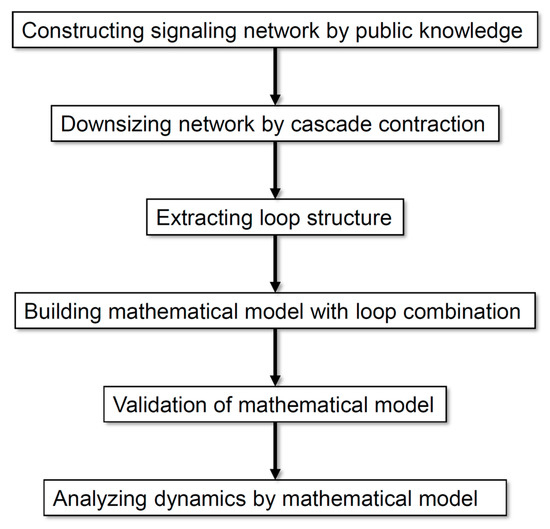
Figure 1.
Flow diagram of the analysis processes employed in this study.
2. Materials and Methods
2.1. Construction of a Neuronal Differentiation Network
To construct the complete signaling network, relations among molecules involved in neuronal differentiation were collected from the literature and pathway databases [16,17,18,19,20,21,22,23], mainly the NCI Pathway Interaction Database [24] and WikiPathways [25]. The switching mechanisms that determine the direction of differentiation, glia, or neurons, are described in the model. The model does not include pathways activated by glial differentiation, but neuronal differentiation, to focus on the differentiation of NSCs into neurons. The signaling networks were constructed using CellDesigner v4.3 [26] by merging binary relations from each data source and were saved in a Systems Biology Markup Language (SBML) format. The complete signaling network was constructed by manually merging all the SBML files. Then, every molecule was color-coded according to its type (receptor, enzyme, transcription factor, or other). Finally, the enzymes and other molecules were divided into active and inactive forms. The graphical representation conformed to the proposed set of symbols in CellDesigner [27].
2.2. Contraction of the Network
To simplify the network without losing the essential loop structures that are important to the original dynamics, the sequences of unidirectional edges (cascade structures) were converted into a single edge between two molecules. The rate of a cascade reaction depends on the rate-limiting reaction. Therefore, each cascade was represented as a single rate-limiting reaction. The contraction was continued manually until a network only consisted of nodes with multiple input/output edges, by removing nodes with both inward and outward degrees of one. After cascade contraction, feedback loop structures were extracted as a core network. At this time, a transcription–translation self-feedback loop, which was initially constructed from one or two molecules, was reconstructed to include three molecules by adding a transcription or translation event, because such events require much more time than signal transduction events, and this investment of time is related to nonlinear dynamics. Finally, to minimize the network size, feedback loops in the core network were contracted again until at least three nodes were formed. After this contraction, the nodes of the contracted cascade were named on the basis of the node name of the original cascade.
2.3. Mathematical Model Construction
The contracted network was converted into a mathematical model (digested model), in which the dynamics of the original network were maintained. The model was constructed using CellDesigner. The contracted network was drawn and kinetics with parameters were assigned to every edge using the SBMLsqueezer [28] plug-in in CellDesigner. In SBMLsqueezer, the ‘Reversibility’ option was set to ‘Use information from SBML’. Every type of enzyme kinetics was set to the Michaelis–Menten equation, which is one of the best-known models of enzyme kinetics. That of transcriptional or translational reactions was set to the Hill equation, which is the simplest way to describe sigmoidal responses. The parameters were estimated in the range of physiologically relevant values which could simulate the experimental results reported by Imayoshi et al. [14]. The range was determined from records in BioNumbers [29,30]. The initial concentration of each protein was set to 1.0 µM because the typical concentration range of a signaling protein is 10 nM–1 µM [31]. For enzymes and other molecules, the concentration of active and inactive forms was set to 0.5 µM each.
2.4. Simulation and Analysis
The dynamics of the digested model were validated by steady-state simulation and parameter analysis. Simulation was performed using CellDesigner, and the analysis was conducted using COPASI 4.14 (Build 89) [32]. The simulation was calculated using SOSlib [33], with the error tolerance set to −6. To simulate the change in dynamics due to the induction of differentiation, an event that perturbed the concentration of NOTCH (differentiation control factor) at an arbitrary time point was configured. The parameter search and bifurcation analysis were conducted using the Parameter Scan function in COPASI, which records the time course of an arbitrary molecule for 500 h while changing an arbitrary parameter or concentration within the defined range. The time course was calculated using LSODA [34], with the following parameters: Integrate Reduced Model, 0; Relative Tolerance, 1e–06; Absolute Tolerance, 1e–12; Max Internal Steps, 10,000. The scope of a parameter scan was set to 0.001–1000, and the range of NOTCH concentrations as a differentiation control factor was set to 0–2.8 µM.
3. Results
3.1. Signaling Network of Neuronal Differentiation
To construct a signaling network of NSC differentiation into a mature neuron, we collected publicly available information about the switch from NOTCH, a molecular marker of differentiation, to neuronal markers such as Tau. The network was constructed by using 54 molecules and contained five modules (Figure 2A). The first module was the differentiation switch from NOTCH. The second module was the expression of transcription factors that are early neural markers [16,17,18,19,20]. The third module was the transition from an immature neuron to a mature neuron. The fourth module was regulation to the gain of mature neuron functions [21,22]. Finally, beta-catenin, a molecule related to the function of mature neurons, controls a bHLH-type transcription factor to adjust differentiation, and was adopted as the fifth module [23]. Converting this entire signaling network into a mathematical model can be challenging because multiple parameters need to be taken into account. Because the network dynamics are controlled by the dynamics of individual loop structures [10], we focused on feedback loops that are important to nonlinear dynamics. For example, a feedback loop may confer the ability of homeostasis, ultra-sensitivity, hysteresis, and bistability [35]. A positive feedback loop is defined as a loop structure containing zero or an even number of negative regulations, and a negative feedback loop is defined as a loop structure containing an odd number of negative regulations (Figure 3A). Although some tools could find a loop structure [36,37], it was difficult to find a large loop structure whose size was over 15 nodes. Therefore, to find a large loop, we need to manually extract a loop structure from complicated and large-scale networks. To facilitate manual loop extraction, we contracted the entire network by cascade contraction until a network only consisted of nodes with multiple input/output edges and extracted feedback loops (Figure 3B, Figure A1, and Table A1). After contraction, feedback loop structures were extracted to obtain the core network of marker molecules, which contained 14 molecules (Figure 2B). Although there were also feed-forward loops in the entire network, they were located downstream of the network and had no connection to marker molecules. Therefore, the feed-forward loops were omitted from the core network. The core network included four feedback loops: (1) a negative-feedback loop formed by HES1 dimerization; (2) a positive-feedback loop between PI3K and aPKC_PAR3_PAR6; (3) a negative-feedback loop between PTEN and GSK3B; and (4) a negative-feedback loop between beta-catenin and HES1. The first three loops have been previously investigated [17,21] (the first one has been especially well-analyzed [38,39]), but the negative-feedback loop between beta-catenin and HES1, which was the largest in our model, has not been focused on. The core network retained the feedback loops of the entire original network, and was thus expected to maintain the original dynamics of marker molecules, HES1 and ASCL1. To analyze the dynamics of the core network, we constructed a mathematical model.
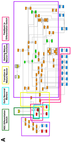
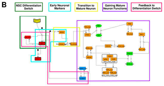
Figure 2.
Signaling network of neural stem cell differentiation based on publicly available data. (A) The entire signaling network. (B) Core signaling network: feedback loops extracted from the entire network. Rectangular nodes are generic proteins. Oval nodes are small molecules. The arrowhead node is a receptor. Dashed-line nodes are active forms. Bold-line nodes are neuronal markers. Node color codes: yellow, receptor; red, transcription factor; orange, enzyme; blue, molecule related to a function of a mature neuron; green, other.
Figure 3.
Feedback loops and contraction. (A) Examples of positive and negative feedback loops. (B) Example of contraction.
3.2. Mathematical Model of the Core Network
Because the core network was still too complex to convert into a mathematical model, we contracted it to the minimum nodes, but maintained the feedback loop structures, including the differentiation switch NOTCH and the indicators of characteristic dynamics before and after differentiation (Figure 4). The self-negative-feedback loop formed by HES1 dimerization—HES1 -> dimer_HES1 -| HES1—was reconstructed as a three-molecule loop by adding mRNA of HES1 (mHES1) as a transcriptional process, because the self-negative feedback loop represented by transcriptional and translational processes was actually composed of the generation of mRNA and translation of mRNA (see Methods for details). Although previous studies introduced a delay into the model [12,13], we convolved the delay with the parameters of the HES1 translation and dimerization steps. The non-delay model of the HES1 self-loop generated oscillations (Figure A2 and Figure A3, and Table A2). To minimize the network, most feedback loops were converted to three-molecule loops by cascade contraction. The contracted cascades were represented with the nodes in our digested model. The names of the nodes were determined based on the name of the first or last node of the original cascade, with the addition of the suffix _ca or _ci. The suffix _ca denoted the active form of a cascade, and _ci denoted the inactive form. The positive-feedback loop between PI3K and aPKC_PAR3_PAR6— PI3K -> PIP3 -> RAP1B -> CDC42_GEF -> CDC42 -> aPKC_PAR3_PAR6 -> TIAM1/2 -> RAC1 -> PI3K—was reconstructed as a three-molecule loop, and the contracted nodes were named PIP_ca (PIP_ci), aPKC_ca (aPKC_ci), and PI3K_ca (PI3K_ci) (Figure A4). The negative-feedback loop between PTEN and GSK3B—PTEN -| PIP3 -> RAP1B -> CDC42_GEF -> CDC42 -> aPKC_PAR3_PAR6 -| GSK3B -| PTEN—was reconstructed as a four-molecule loop, and the contracted nodes were named PTEN_ca (PTEN_ci) and GSK3B_ca (GSK3B_ci) (Figure A5). The negative-feedback loop between beta-catenin and HES1—HES1 -| NEUROG2 -| RHOA -> Rho_kinase -> PTEN -| PIP3 -> RAP1B -> CDC42_GEF -> CDC42 -> aPKC_PAR3_PAR6 -| GSK3B -| B-catenin -> HES1—was reconstructed as a six-molecule loop (Figure A6). This network was translated into a deterministic mathematical digested model governed by the Hill equation and Michaelis–Menten kinetics (Table 1). The final digested model was constructed using nine molecules (15 nodes) and 20 reactions, which reduced the network size by 84.3% in comparison with the entire signaling network. Thereafter, the dynamics of neuronal differentiation were analyzed by using the digested model. The model is provided as an SBML file in the Supplementary Materials.
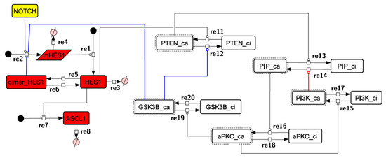
Figure 4.
Diagram of the toy model. The model consists of multiple feedback loops extracted from the core signaling network. The red edge is a component of a positive feedback loop. Blue edges are components of negative feedback loops. Node color codes: yellow, receptor; red, transcription factor; white, contracted node.

Table 1.
Differential equations of the toy model.
3.3. Simulation of the Oscillatory Dynamics
To simulate the oscillatory state of HES1 and ASCL1 in undifferentiated NSCs as a basal condition (as reported by Imayoshi et al. [14]), the digested model was investigated using an oscillatory parameter set. The ranges of 40 parameters (Table 2) allowed the model to maintain oscillations. To check whether these parameter values were physiologically relevant, we compared them to the general parameter values of Michaelis–Menten kinetics based on the BioNumbers database [29]. The minimal values of the parameters in the Hill equation that allowed the expected behaviors of the model to be reconstructed were chosen. Almost all parameters of enzymes, except kM_re2_s24 and kM_re2_s9, exhibit kM values above 0.1 µM [30], and almost all of the kM values in the model were above 0.1 µM in the oscillatory range. The maximum (37,596,000 h−1) and minimum (264 h−1) Kcat values were acquired from 27 records for mammals in BioNumbers; all Kcat values in the model were within this range. Detailed records are provided as an Excel file in the Supplementary Materials. These data indicated that the oscillatory state could be established under physiologically relevant conditions. The model could simulate the HES1 and ASCL1 oscillation within the 2.5 h period reported by Imayoshi et al. [14] in the undifferentiated state as the basal condition (Figure 5A and Figure A7).
Table 2.
Oscillation parameter ranges.
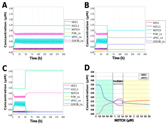
Figure 5.
Simulation of the toy model. (A) Basic condition with a 2.5 h period. (B) Negative and (C) positive perturbation of the NOTCH concentration at 50 h. (D) Bifurcation analysis of the HES1 and ASCL1 concentration dependence on the NOTCH concentration. Background colors show cell differentiation state; green, neuron; yellow, astrocyte.
3.4. Model Validation
During neural differentiation, the characteristic dynamics of the transition from the oscillatory to the non-oscillatory state of HES1 and ASCL1 are controlled by the concentration of NOTCH [14]. In the non-oscillatory state after differentiation, the concentration of ASCL1 was higher than that of HES1 in a neuron, whereas the concentration of HES1 was higher than that of ASCL1 in an astrocyte. To simulate the physiological condition at the initiation of neuronal differentiation, we set a low concentration of NOTCH during simulation. As a result, ASCL1 became dominant in a non-oscillatory state. At the same time, the concentration of GSK3B_ca, which included GSK3B (a negative regulator [21]), decreased and the concentrations of aPKC_ca, which included aPKC_PAR3_PAR6, and PI3K_ca, which included PI3K (positive regulators [21]), increased (Figure 5B). These results agreed with previously reported experimental results on neuronal differentiation [14,21]. Conversely, we set a high concentration of NOTCH and executed the simulation. The oscillation of concentrations of HES1 and ASCL1 disappeared and the equilibrium concentration of HES1 became higher than that of ASCL1 (Figure 5C). This result agrees with the previously reported initiation of glial differentiation [14]. Both ASCL1 and HES1 maintained oscillations at physiologically relevant NOTCH concentrations in an NSC (Figure 5D) [31]. This NOTCH-dependent dynamic transition was consistent with the experimental results of Imayoshi et al. [14]. We also simulated the overexpression and knockdown of the Id2 gene, which encodes an inhibitor of HES1 dimerization [15]. The knockdown of Id2 promotes neuronal differentiation by suppressing HES1 and enhancing ASCL1 expression, and the overexpression of Id2 inhibits neuronal differentiation by enhancing HES1 and suppressing ASCL1 expression [15]. To simulate the inhibition of HES1 dimerization by Id2, an inhibition parameter, kSm_Id (an indicator of the amount of Id2), was introduced into equations 1 and 3 (Table 1) to obtain equations 1′ and 3′ (Table 3), respectively. When Id2 knockdown was simulated by setting kSm_Id to 0.1, oscillations disappeared, and a neuronal differentiation state with ASCL1 domination was observed at each NOTCH concentration (Figure 6A). When Id2 overexpression was simulated by setting kSm_Id to 10, oscillations also disappeared, and a non-neuronal differentiation state with HES1 domination was observed at NOTCH concentrations over 0.7 µM (Figure 6B). Therefore, the digested model maintained the original dynamics of the entire network.
Table 3.
Differential equations of a model with an incorporated inhibition of HES1 dimerization by Id2.
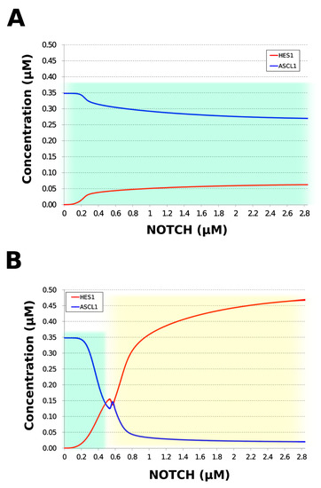
Figure 6.
Simulation of HES1 and ASCL1 concentrations under the Id2 gene knockdown or overexpression conditions. (A) Id2 gene knockdown with kSm_Id = 0.1. (B) Id2 gene overexpression with kSm_Id = 10. Background colors show cell differentiation state; green, neuron; yellow, astrocyte.
3.5. Model Analysis
We analyzed the contribution of each loop to the results of simulation of NOTCH responsiveness by bifurcation analysis. To simulate a loss-of-function mutation that inhibits the self-feedback regulation of HES1, we collapsed the self-feedback loop of HES1 in our model and executed the simulation (Figure A8). When the loop was collapsed by changing equation 2 to equation 2’ (Table 4), the oscillatory state, which is important for maintaining the undifferentiated state, disappeared. At the same time, the ASCL1-dominant state, which is important for differentiation into neurons, became narrower with rapid HES1 upregulation (Figure 7A). Therefore, this loop is required to maintain the oscillatory state and ASCL1-dominant state. This result agreed with the reported result of HES1 inhibition by the overexpression of Id2 [15]. To simulate the specific inhibition of the effect of GSK3B on PTEN, we collapsed the negative feedback loop between GSK3B and PTEN by changing equations 5 and 6 to equations 5’ and 6’, respectively (Table 4, Figure A9). The oscillatory state shifted to higher NOTCH concentrations (Figure 7B), which means that this loop was involved in the sensitivity of oscillations to the NOTCH concentration. GSK3B may promote or inhibit NOTCH signaling under different conditions, depending on the loops involved [40,41,42,43]. The dichotomic characteristics of GSK3B may enable it to arbitrate the response to NOTCH, given that our simulation suggested that the GSK3B−PTEN loop regulated the sensitivity of oscillations to NOTCH. To simulate the specific inhibition of the effect of PI3K to PIP2, we collapsed the positive feedback loop between aPKC_PAR3_PAR6 and PI3K by changing equations 7 and 8 to equations 7’ and 8’, respectively (Table 4, Figure A10). The relative changes in HES1 and ASCL1 concentrations with the NOTCH concentration were maintained, but the oscillatory state disappeared (Figure 7C). Therefore, the aPKC_PAR3_PAR6−PI3K loop is required to maintain the oscillatory state. We estimated the effect of the collapse of this loop by inhibiting PI3K. A PI3K inhibitor, LY294002, inhibits the proliferation of neural progenitor cells [23,43]; our result agreed with the published data. To simulate the specific inhibition of the effect of beta-catenin on HES1, we collapsed the negative feedback loop between beta-catenin and HES1 by changing equation 2 to equation 2’’ (Table 4, Figure A11). The oscillations disappeared and the ASCL1-dominant state became narrower (Figure 7D), indicating that this loop is required for maintaining oscillations and upregulating ASCL1 at low concentrations of NOTCH. The collapse of this loop equals beta-catenin inhibition, which represses the proliferation of neural progenitor cells and accelerates glial differentiation [44,45]. Glial differentiation is induced without oscillation under ASCL1 repression [14]. Our result that the collapse of this loop leads to ASCL1 repression is consistent with the reported acceleration of glial differentiation by beta-catenin inhibition. These results suggest that multiple feedback loops are essential for the characteristic dynamics of neural differentiation.
Table 4.
Differential equations of models with the feedback loop removed.
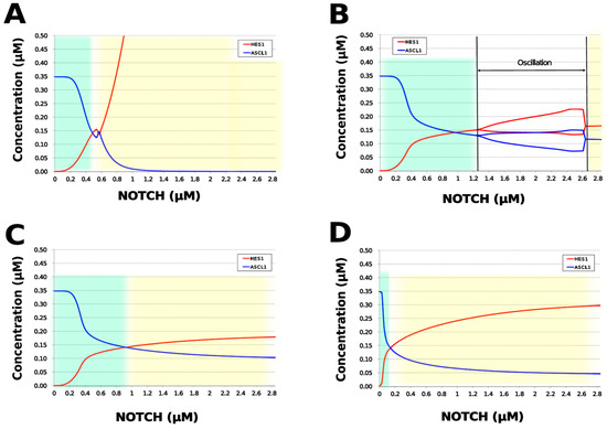
Figure 7.
Bifurcation analysis of the HES1 and ASCL1 concentration dependence on the NOTCH concentration when each feedback loop is collapsed. (A) Collapsed HES1 self-feedback loop. (B) Collapsed negative-feedback loop between GSK3B and PTEN. (C) Collapsed positive-feedback loop between aPKC_PAR3_PAR6 and PI3K. (D) Collapsed negative-feedback loop between beta-catenin and HES1. Background colors show cell differentiation state; green, neuron; yellow, astrocyte.
4. Discussion
We generated an NSC differentiation network containing four feedback loops on the basis of publicly available data. Our digested model was constructed through cascade contraction of the comprehensive regulatory network with the preservation of feedback loops. Three types of HES1 and ASCL1 states regulated by the NOTCH concentration were consistent with the NOTCH-dependent neural differentiation suggested by Imayoshi et al. [14]. Although experimental data show complex waveforms of HES1 and ASCL1, we simulated the main-frequency waves, which have a period of 2 to 3 h [14], and analyzed the dynamics of the transition from the oscillatory to the non-oscillatory state qualitatively using a digested model. The results of the simulation of GSK3B, aPKC_PAR3_PAR6, and PI3K, represented as GSK3B_ca, aPKC_ca, and PI3K_ca in the digested model, respectively, are consistent with previous experimental results [21] (Figure 5B,C). The results of the simulation of Id2 knockdown or overexpression are also consistent with experimental results [15]. Therefore, our digested model could adequately simulate the dynamics not only of HES1 and ASCL1, but also of other molecules. Our model suggests that three loops (HES1 negative self-feedback, positive feedback between aPKC_PAR3_PAR6 and PI3K, and negative feedback between GSK3B and HES1) are important for maintaining undifferentiated state oscillations. Our simulation result showed that inhibition of the HES1 self-feedback loop caused the disappearance of its oscillatory expression (Figure 7A). At the same time, the ASCL1-dominant condition, which is equal to the neuronal differentiation-dominant condition, becomes narrower. This means that the inhibition of the HES1 self-feedback loop could suppress the differentiation of NSCs. A previous study experimentally showed that the inhibition of HES1 by overexpression of the id protein caused the inhibition of differentiation [15]. Therefore, the result of our simulation was consistent with this previous experimental knowledge. We suggest that the negative-feedback loop between beta-catenin and HES1 in the comprehensive regulatory network is also important because of its greatest contribution to the characteristic dynamics (Figure 7D). A relation between beta-catenin and HES1 plays a role in tumorigenesis [46]. As HES1 controls cancer stem cells [47], the negative feedback loop that has not been focused on may be related to the proliferation and differentiation of cancer stem cells. It is expected that a further experimental study, such as perturbating the loop by knock down, will reveal detailed mechanisms of neural differentiation. These findings could only be produced by using the analysis based on a large-scale regulatory network, thus highlighting the effectiveness of our approach.
We demonstrated that focusing on feedback loop structures instead of the whole network when constructing a model was sufficient for producing data in agreement with experimental results. Our approach could be applied to an analysis of various biochemical networks by simulation. By streamlining large-scale regulatory network construction, our approach could help to analyze various biological phenomena, such as cell differentiation, cell division, or pathogenesis. However, the large-scale regulatory network will probably be insufficient and heterogeneous when it is constructed using the available data alone. To overcome this false-negative problem (the relations that exist, but cannot be detected), many data-driven network reconstruction methods have been developed. These statistical approaches are mainly classified under two categories: expression-based [48] and sequence-based [49]. Although the methods of both categories can reveal undiscovered relations that cannot be inferred manually, the reconstructed network includes many false-positive regulations. A nonlinear model intrinsically causes complex behavior. With an increase in the number of false-positive regulations, an increase in the number of nonlinearities becomes avoidable. Based on this mathematical background, a model with a high number of false-positive regulations seemingly generates the real behavior, but is different from the real system. Therefore, it is desirable to build a mathematical model only from reliable elements. The addition of false-positive regulation to the model could have a considerable effect and complicate the conversion of a data-driven network into a mathematical model. Currently, the manual methods are better than the data-driven methods for the construction of a mathematical model.
Our large-scale regulatory network of neuronal differentiation may lack some components and thus may not completely represent neuronal differentiation. In our network, ASCL1 is directly affected by HES1; ASCL1 oscillation controls proliferation and differentiation [14] and affects NOTCH receptors of adjacent cells via the activation of DLL [50]. Neural differentiation is also affected by adjacent cells [51]. We excluded this information because we focused on the dynamics of a single cell. To reveal the entire mechanism of neural differentiation, adding a path to adjacent cells, for instance via DLL, might be required. The analysis of multiple cells might provide a model that can simulate dynamics other than state transitions. The concentrations of both HES1 and ASCL1 decrease in a non-oscillatory state when an NSC differentiates into an oligodendrocyte [14]. To simulate this transition, we need to add a signaling pathway focusing on the oligodendrocyte marker OLIG2, which oscillates with a period of 400 min in NSCs [14]. This period is much longer than that of HES1 or ASCL1, and the dispersion of oscillation is very high. Therefore, OLIG2 regulation might involve a delay mechanism to elongate the period and a mechanism to amplify dispersion. Recently, a similar method was used to analyze oligodendrocyte differentiation [52]. Similar to our study, the authors used a manual method to construct a network; however, they also introduced publicly available interaction data from omics databases. In comparison with our method, this approach may reduce the number of false-negative interactions. On the other hand, the study [52] only focused on two- to four-node feedback loops. Our contraction method may detect a larger regulatory system of oligodendrocyte differentiation. The complete mechanism of neural differentiation may be simulated by integrating this information and methods. Our model can simulate the dynamics of NSC-to-neuron transition and exemplify the reverse transition by increasing the concentration of NOTCH, but differentiation is mostly irreversible. Therefore, it is difficult to validate the results of reversing from a neuron to an NSC. Some hypotheses suggest the core factors of differentiation that also inhibit reprogramming [53] or control the mechanisms generated by neurogenic niches [54]. Specific network structures such as positive feedbacks or micro-environmental factors may be important for hysteresis in differentiation, and a more detailed, larger network needs to be analyzed.
There exist some network reduction approaches, but some of them are limited in terms of the preservability of original dynamics [6,7]. Kernel Identification [8] is one of the methods employed to preserve the network dynamics; however, the preservability is only validated with Boolean models. Because we aimed to maintain the network dynamics at the level of ordinary differential equations, we concentrated on extracting loops. We did not modify the network, except for cascades as the target of reduction, instead of applying the previous work. Practically, network reduction by Kernel Identification may produce a similar contracted network and will be advantageous when the network is larger than in this case.
To simulate more realistic behaviors of biological cells, highly crowded and inhomogeneous environments should be considered. The use of fractional derivatives has been well-evaluated in the usage of visco-elastic processes of soft materials [55], and recently, they have started to apply more biological targets [56,57,58,59]. Our mathematical model of neural differentiation is also expected to become more realistic by fractional derivatives instead of classical integer derivatives. Although we focused on NOTCH signaling in this study, our network also includes FGF as another input signal. An analysis of the behavior of the network stimulated with FGF may show variate responses and as a result, may reveal other mechanisms of neural differentiation. Although the core network did not include a feed-forward loop, a feed-forward loop accelerates the response time of a system and achieves cell state transition rapidly. Because the cellular state transition obtained by NOTCH signaling is also known to be accelerated by a feed-forward loop [60], a feed-forward loop may exist upstream of the core network. Our method can be used to analyze the dynamics of a new large-scale regulatory network when new information becomes available.
5. Conclusions
The construction of a large-scale regulatory network of neuronal differentiation based on publicly available data led to the identification of a new feedback loop structure, which we expect regulates differentiation. The large-scale regulatory network was modeled mathematically after network contraction, and the extracted digested model simulated the characteristic dynamics of HES1 and ASCL1, which were suggested to be regulated by multiple loops. More information about neural differentiation and further analyses focused on loop structures will deepen our understanding of the mechanism of neural differentiation. Our approach is applicable to other biological models for which detailed mechanisms are unknown.
Supplementary Materials
Further details on the digested model and data from BioNumbers are available at https://www.mdpi.com/2227-9717/8/2/166/s1.
Author Contributions
Conceived and designed the experiments: T.I., T.G.Y., N.F.H., A.F., and K.Y. Performed the analyses: T.I., R.T., T.G.Y., and T.H. Wrote the paper: T.I., T.G.Y., N.F.H., and A.F. Critical advice on the manuscript: T.H. and K.Y. All authors have read and agreed to the published version of the manuscript.
Funding
Sumitomo Dainippon Pharma Co., Ltd. provided support in the form of salaries for T. Iwasaki and K. Yamazaki and as part of the research budget to N. Hiroi. The company did not play any role in the study design, data collection, or analysis. The specific roles of these authors are described in the Authors’ Contributions section. This work was supported by the Japan Society for the Promotion of Science (JSPS), a Grant-in-Aid for Scientific Research (Kiban C) 15K06925 awarded to N. Hiroi.
Acknowledgments
We thank Tetsuya J. Kobayashi (Institute of Industrial Science, the University of Tokyo) for his constructive comments and encouragement. We thank ELSS (Tsukuba, Japan) for their critical advice on English usage and proofreading of the manuscript.
Conflicts of Interest
The authors declare no conflicts of interest.
Appendix A. Supporting Figures and Tables

Figure A1.
Cascade-contracted network. To find the feedback loop, the whole signaling network was contracted by cascade contraction.

Figure A2.
Diagram of the HES1 negative self-feedback loop model without delay. The model consists of an HES1 negative self-feedback loop with three nodes without delay. The red edge represents positive regulation. The blue edge represents negative regulation.

Figure A3.
Simulation result of the HES1-loop model. The model could simulate the oscillatory state with a period of almost 2 hours. The following parameters were used: k3 = 0.00129, k3r = 0.0232, kg2 = 4.25, nmre1s9 = 5, kSmre1s9 = 0.00228, kg1 = 3.24, ks3d = 0.0258, and ks2d = 0.0355.

Figure A4.
Diagram of the positive-feedback loop between PI3K and aPKC_PAR3_PAR6. (A) The positive-feedback loop in the whole signaling network. (B) The contracted positive-feedback loop in the toy model. Red edges represent positive regulations. Background colors show correspondence relationships between before and after contraction.

Figure A5.
Diagram of the negative-feedback loop between PTEN and GSK3B. (A) The negative-feedback loop in the whole signaling network. (B) The contracted negative-feedback loop in the toy model. Red edges represent positive regulations. Blue edges represent negative regulations. Background color shows correspondence relationship between before and after contraction.

Figure A6.
Diagram of negative-feedback loop between beta-catenin and HES1. (A) The negative-feedback loop in the whole signaling network. (B) The contracted negative-feedback loop in the toy model. Red edges represent positive regulations. Blue edges represent negative regulations. Background colors show correspondence relationships between before and after contraction.

Figure A7.
Simulation result of all species.

Figure A8.
Diagram of the collapsed model of the HES1 self-feedback loop.

Figure A9.
Diagram of the collapsed model of the negative-feedback loop between GSK3B and PTEN.

Figure A10.
Diagram of the collapsed model of the positive-feedback loop between aPKC_PAR3_PAR6 and PI3K.

Figure A11.
Diagram of the collapsed model of the negative-feedback loop between beta-catenin and HES1.
Table A1.
Nodes removed by the contraction process.
Table A1.
Nodes removed by the contraction process.
| Node Name | Reason | Integrated To (Identifier in the Toy Model) |
|---|---|---|
| NEUROG2 | Cascade (whole signaling network) | Rho_kinase |
| MLC | Cascade (whole signaling network) | Rho_kinase |
| RhoA | Cascade (whole signaling network) | Rho_kinase |
| RAP1B | Cascade (whole signaling network) | PIP3 |
| CDC42_GEF | Cascade (whole signaling network) | PIP3 |
| Cofilin | Cascade (whole signaling network) | PAK |
| LIMK | Cascade (whole signaling network) | PAK |
| Stathmin | Cascade (whole signaling network) | PAK |
| N_WASP | Cascade (whole signaling network) | CDC42 |
| MRCK | Cascade (whole signaling network) | CDC42 |
| KLC | Cascade (whole signaling network) | GSK3B |
| APC | Cascade (whole signaling network) | GSK3B |
| b-catenin | Cascade (whole signaling network) | GSK3B |
| mTOR | Cascade (whole signaling network) | PIP3 |
| RHEB | Cascade (whole signaling network) | PIP3 |
| PDK1 | Cascade (whole signaling network) | PIP3 |
| ILK | Cascade (whole signaling network) | PIP3 |
| AKT | Cascade (whole signaling network) | PIP3 |
| L1 | Cascade (whole signaling network) | RAS |
| CREB | Cascade (whole signaling network) | RAS |
| MAPKAP_K1 | Cascade (whole signaling network) | RAS |
| MAPK | Cascade (whole signaling network) | RAS |
| MEK | Cascade (whole signaling network) | RAS |
| RAF | Cascade (whole signaling network) | RAS |
| MARK2 | Cascade (whole signaling network) | aPKC_PAR3_PAR6 |
| Arp2/3 | Feedback loop extraction | - |
| IQGAP3 | Feedback loop extraction | - |
| PAK | Feedback loop extraction | - |
| p35/CDK5 | Feedback loop extraction | - |
| SRA1_WAVE1 | Feedback loop extraction | - |
| MAP1B | Feedback loop extraction | - |
| Tau | Feedback loop extraction | - |
| CRMP-2 | Feedback loop extraction | - |
| RAS | Parameterization | - |
| Rho_kinase | Cascade (core network) | PTEN_ca (s22) |
| TIAM1/2 | Cascade (core network) | PI3K_ca (s20) |
| RAC1 | Cascade (core network) | PI3K_ca (s20) |
| PIP3 | Cascade (core network) | PIP_ca (s16) |
| GSK3B | Cascade (core network) | GSK3B_ca (s24) |
| PTEN | Cascade (core network) | PTEN_ca (s22) |
| aPKC_PAR3_PAR6 | Cascade (core network) | aPKC_ca (s18) |
Table A2.
Differential equations of the HES1 self-loop model.
Table A2.
Differential equations of the HES1 self-loop model.
| Equation No. | Differential equations |
|---|---|
| 1 | |
| 2 | |
| 3 |
References
- Karr, J.R.; Sanghvi, J.C.; Macklin, D.N.; Gutschow, M.V.; Jacobs, J.M.; Bolival, B., Jr.; Assad-Garcia, N.; Glass, J.I.; Covert, M.W. A whole-cell computational model predicts phenotype from genotype. Cell 2012, 150, 389–401. [Google Scholar] [CrossRef]
- Vignes, M.; Vandel, J.; Allouche, D.; Ramadan-Alban, N.; Cierco-Ayrolles, C.; Schiex, T.; Mangin, B.; de Givry, S. Gene regulatory network reconstruction using Bayesian networks, the Dantzig Selector, the Lasso and their meta-analysis. PLoS ONE 2011, 6, e29165. [Google Scholar] [CrossRef]
- Chai, L.E.; Loh, S.K.; Low, S.T.; Mohamad, M.S.; Deris, S.; Zakaria, Z. A review on the computational approaches for gene regulatory network construction. Comput. Biol. Med. 2014, 48, 55–65. [Google Scholar] [CrossRef]
- Park, Y.; Kellis, M. Deep learning for regulatory genomics. Nat. Biotechnol. 2015, 33, 825–826. [Google Scholar] [CrossRef]
- Karr, J.R.; Williams, A.H.; Zucker, J.D.; Raue, A.; Steiert, B.; Timmer, J.; Kreutz, C.; Wilkinson, S.; Allgood, B.A.; Bot, B.M.; et al. Summary of the DREAM8 Parameter Estimation Challenge: Toward Parameter Identification for Whole-Cell Models. PLoS Comput. Biol. 2015, 11, e1004096. [Google Scholar] [CrossRef]
- Itzkovitz, S.; Levitt, R.; Kashtan, N.; Milo, R.; Itzkovitz, M.; Alon, U. Coarse-graining and self-dissimilarity of complex networks. Phys. Rev. E Stat. Nonlinear Soft Matter Phys. 2005, 71 Pt 2, 016127. [Google Scholar] [CrossRef]
- Kim, D.H.; Noh, J.D.; Jeong, H. Scale-free trees: The skeletons of complex networks. Phys. Rev. E Stat. Nonlinear Soft Matter Phys. 2004, 70 Pt 2, 046126. [Google Scholar] [CrossRef]
- Kim, J.R.; Kim, J.; Kwon, Y.K.; Lee, H.Y.; Heslop-Harrison, P.; Cho, K.H. Reduction of complex signaling networks to a representative kernel. Sci. Signal. 2011, 4, ra35. [Google Scholar] [CrossRef]
- Milo, R.; Shen-Orr, S.; Itzkovitz, S.; Kashtan, N.; Chklovskii, D.; Alon, U. Network motifs: Simple building blocks of complex networks. Science 2002, 298, 824–827. [Google Scholar] [CrossRef]
- Riccione, K.A.; Smith, R.P.; Lee, A.J.; You, L. A synthetic biology approach to understanding cellular information processing. ACS Synth. Biol. 2012, 1, 389–402. [Google Scholar] [CrossRef][Green Version]
- Louvi, A.; Artavanis-Tsakonas, S. Notch signalling in vertebrate neural development. Nat. Rev. Neurosci. 2006, 7, 93–102. [Google Scholar] [CrossRef]
- Monk, N.A. Oscillatory expression of Hes1, p53, and NF-kappaB driven by transcriptional time delays. Curr. Biol. 2003, 13, 1409–1413. [Google Scholar] [CrossRef]
- Zeiser, S.; Müller, J.; Liebscher, V. Modeling the Hes1 oscillator. J. Comput. Biol. 2007, 14, 984–1000. [Google Scholar] [CrossRef]
- Imayoshi, I.; Isomura, A.; Harima, Y.; Kawaguchi, K.; Kori, H.; Miyachi, H.; Fujiwara, T.; Ishidate, F.; Kageyama, R. Oscillatory control of factors determining multipotency and fate in mouse neural progenitors. Science 2013, 342, 1203–1208. [Google Scholar] [CrossRef]
- Bai, G.; Sheng, N.; Xie, Z.; Bian, W.; Yokota, Y.; Benezra, R.; Kageyama, R.; Guillemot, F.; Jing, N. Id sustains Hes1 expression to inhibit precocious neurogenesis by releasing negative autoregulation of Hes1. Dev. Cell 2007, 13, 283–297. [Google Scholar] [CrossRef]
- Kageyama, R.; Ohtsuka, T.; Hatakeyama, J.; Ohsawa, R. Roles of bHLH genes in neural stem cell differentiation. Exp. Cell Res. 2005, 306, 343–348. [Google Scholar] [CrossRef]
- Kageyama, R.; Ohtsuka, T.; Kobayashi, T. Roles of Hes genes in neural development. Dev. Growth Differ. 2008, 50 (Suppl. S1), S97–S103. [Google Scholar] [CrossRef]
- Seki, T.; Sawamoto, K.; Parent, J.M.; Alvarez-Buylla, A. (Eds.) Neurogenesis in the Adult Brain; Springer: Tokyo, Japan, 2011; Volume 1. [Google Scholar]
- Roybon, L.; Mastracci, T.L.; Ribeiro, D.; Sussel, L.; Brundin, P.; Li, J.Y. GABAergic differentiation induced by Mash1 is compromised by the bHLH proteins Neurogenin2, NeuroD1, and NeuroD2. Cereb. Cortex 2010, 20, 1234–1244. [Google Scholar] [CrossRef]
- Bhat, K.M.; Maddodi, N.; Shashikant, C.; Setaluri, V. Transcriptional regulation of human MAP2 gene in melanoma: Role of neuronal bHLH factors and Notch1 signaling. Nucleic Acids Res. 2006, 34, 3819–3832. [Google Scholar] [CrossRef]
- Arimura, N.; Kaibuchi, K. Neuronal polarity: From extracellular signals to intracellular mechanisms. Nat. Rev. Neurosci. 2007, 8, 194–205. [Google Scholar] [CrossRef]
- Hand, R.; Bortone, D.; Mattar, P.; Nguyen, L.; Heng, J.I.; Guerrier, S.; Boutt, E.; Peters, E.; Barnes, A.P.; Parras, C.; et al. Phosphorylation of Neurogenin2 specifies the migration properties and the dendritic morphology of pyramidal neurons in the neocortex. Neuron 2005, 48, 45–62. [Google Scholar] [CrossRef]
- Shimizu, T.; Kagawa, T.; Inoue, T.; Nonaka, A.; Takada, S.; Aburatani, H.; Taga, T. Stabilized beta-catenin functions through TCF/LEF proteins and the Notch/RBP-Jkappa complex to promote proliferation and suppress differentiation of neural precursor cells. Mol. Cell Biol. 2008, 28, 7427–7441. [Google Scholar] [CrossRef]
- Schaefer, C.F.; Anthony, K.; Krupa, S.; Buchoff, J.; Day, M.; Hannay, T.; Buetow, K.H. PID: The Pathway Interaction Database. Nucleic Acids Res. 2009, 37, D674–D679. [Google Scholar] [CrossRef]
- Kelder, T.; van Iersel, M.P.; Hanspers, K.; Kutmon, M.; Conklin, B.R.; Evelo, C.T.; Pico, A.R. WikiPathways: Building research communities on biological pathways. Nucleic Acids Res. 2012, 40, D1301–D1307. [Google Scholar] [CrossRef]
- Funahashi, A.; Matsuoka, Y.; Jouraku, A.; Morohashi, M.; Kikuchi, N.; Kitano, H. CellDesigner 3.5: A Versatile Modeling Tool for Biochemical Networks. Proc. IEEE 2008, 96, 1254–1265. [Google Scholar] [CrossRef]
- Kitano, H.; Funahashi, A.; Matsuoka, Y.; Oda, K. Using process diagrams for the graphical representation of biological networks. Nat. Biotechnol. 2005, 23, 961–966. [Google Scholar] [CrossRef]
- Dräger, A.; Hassis, N.; Supper, J.; Schröder, A.; Zell, A. SBMLsqueezer: A CellDesigner plug-in to generate kinetic rate equations for biochemical networks. BMC Syst. Biol. 2008, 2, 39. [Google Scholar] [CrossRef]
- Milo, R.; Jorgensen, P.; Moran, U.; Weber, G.; Springer, M. BioNumbers--the database of key numbers in molecular and cell biology. Nucleic Acids Res. 2010, 38, D750–D753. [Google Scholar] [CrossRef]
- Bar-Even, A.; Noor, E.; Savir, Y.; Liebermeister, W.; Davidi, D.; Tawfik, D.S.; Milo, R. The moderately efficient enzyme: Evolutionary and physicochemical trends shaping enzyme parameters. Biochemistry 2011, 50, 4402–4410. [Google Scholar] [CrossRef]
- Legewie, S.; Herzel, H.; Westerhoff, H.V.; Blüthgen, N. Recurrent design patterns in the feedback regulation of the mammalian signalling network. Mol. Syst. Biol. 2008, 4, 190. [Google Scholar] [CrossRef]
- Hoops, S.; Sahle, S.; Gauges, R.; Lee, C.; Pahle, J.; Simus, N.; Singhal, M.; Xu, L.; Mendes, P.; Kummer, U. COPASI-A COmplex PAthway SImulator. Bioinformatics 2006, 22, 3067–3074. [Google Scholar] [CrossRef]
- Machné, R.; Finney, A.; Müller, S.; Lu, J.; Widder, S.; Flamm, C. The SBML ODE Solver Library: A native API for symbolic and fast numerical analysis of reaction networks. Bioinformatics 2006, 22, 1406–1407. [Google Scholar] [CrossRef]
- Petzold, L. Automatic selection of methods for solving stiff and nonstiff systems of ordinary differential equations. SIAM J. Sci. Stat. Comput. 1983, 4, 136–148. [Google Scholar] [CrossRef]
- Eberhardt, M.; Lai, X.; Tomar, N.; Gupta, S.; Schmeck, B.; Steinkasserer, A.; Schuler, G.; Vera, J. Third-kind encounters in biomedicine: Immunology meets mathematics and informatics to become quantitative and predictive. Methods Mol. Biol. 2016, 1386, 135–179. [Google Scholar]
- Trinh, H.C.; Le, D.H.; Kwon, Y.K. PANET: A GPU-based tool for fast parallel analysis of robustness dynamics and feed-forward/feedback loop structures in large-scale biological networks. PLoS ONE 2014, 9, e103010. [Google Scholar] [CrossRef]
- Patra, S.; Mohapatra, A. Application of dynamic expansion tree for finding large network motifs in biological networks. PeerJ. 2019, 7, e6917. [Google Scholar] [CrossRef]
- Hirata, H.; Yoshiura, S.; Ohtsuka, T.; Bessho, Y.; Harada, T.; Yoshikawa, K.; Kageyama, R. Oscillatory expression of the bHLH factor Hes1 regulated by a negative feedback loop. Science 2002, 298, 840–843. [Google Scholar] [CrossRef]
- Kageyama, R.; Ohtsuka, T.; Kobayashi, T. The Hes gene family: Repressors and oscillators that orchestrate embryogenesis. Development 2007, 134, 1243–1251. [Google Scholar] [CrossRef]
- Foltz, D.R.; Santiago, M.C.; Berechid, B.E.; Nye, J.S. Glycogen synthase kinase-3beta modulates notch signaling and stability. Curr. Biol. 2002, 12, 1006–1011. [Google Scholar] [CrossRef]
- Guha, S.; Cullen, J.P.; Morrow, D.; Colombo, A.; Lally, C.; Walls, D.; Redmond, E.M.; Cahill, P.A. Glycogen synthase kinase 3 beta positively regulates Notch signaling in vascular smooth muscle cells: Role in cell proliferation and survival. Basic Res. Cardiol. 2011, 106, 773–785. [Google Scholar] [CrossRef]
- Jin, Y.H.; Kim, H.; Oh, M.; Ki, H.; Kim, K. Regulation of Notch1/NICD and Hes1 expressions by GSK-3alpha/beta. Mol. Cells 2009, 27, 15–19. [Google Scholar] [CrossRef]
- Kim, W.Y.; Wang, X.; Wu, Y.; Doble, B.W.; Patel, S.; Woodgett, J.R.; Snider, W.D. GSK-3 is a master regulator of neural progenitor homeostasis. Nat. Neurosci. 2009, 12, 1390–1397. [Google Scholar] [CrossRef]
- Ye, F.; Chen, Y.; Hoang, T.; Montgomery, R.L.; Zhao, X.H.; Bu, H.; Hu, T.; Taketo, M.M; van Es, J.H.; Clevers, H.; et al. HDAC1 and HDAC2 regulate oligodendrocyte differentiation by disrupting the beta-catenin-TCF interaction. Nat. Neurosci. 2009, 12, 829–838. [Google Scholar] [CrossRef]
- Zhang, C.; Zhang, Z.; Shu, H.; Liu, S.; Song, Y.; Qiu, K.; Yang, H. The modulatory effects of bHLH transcription factors with the Wnt/beta-catenin pathway on differentiation of neural progenitor cells derived from neonatal mouse anterior subventricular zone. Brain Res. 2010, 1315, 1–10. [Google Scholar] [CrossRef]
- Peignon, G.; Durand, A.; Cacheux, W.; Ayrault, O.; Terris, B.; Laurent-Puig, P.; Shroyer, N.F.; Van Seuningen, I.; Honjo, T.; Perret, C.; et al. Complex interplay between b-catenin signalling and Notch effectors in intestinal tumorigenesis. Gut 2011, 60, 166–176. [Google Scholar] [CrossRef]
- Liu, Z.H.; Dai, X.M.; Du, B. Hes1: A key role in stemness, metastasis and multidrug resistance. Cancer Biol. Ther. 2015, 16, 353–359. [Google Scholar] [CrossRef]
- Chasman, D.; Fotuhi Siahpirani, A.; Roy, S. Network-based approaches for analysis of complex biological systems. Curr. Opin. Biotechnol. 2016, 39, 157–166. [Google Scholar] [CrossRef]
- McLeay, R.C.; Bailey, T.L. Motif Enrichment Analysis: A unified framework and an evaluation on ChIP data. BMC Bioinform. 2010, 11, 165. [Google Scholar] [CrossRef]
- Morimoto, M.; Nishinakamura, R.; Saga, Y.; Kopan, R. Different assemblies of Notch receptors coordinate the distribution of the major bronchial Clara, ciliated and neuroendocrine cells. Development 2012, 139, 4365–4373. [Google Scholar] [CrossRef]
- Ramos, C.; Rocha, S.; Gaspar, C.; Henrique, D. Two Notch ligands, Dll1 and Jag1, are differently restricted in their range of action to control neurogenesis in the mammalian spinal cord. PLoS ONE 2010, 5, e15515. [Google Scholar] [CrossRef][Green Version]
- Cantone, M.; Küspert, M.; Reiprich, S.; Lai, X.; Eberhardt, M.; Göttle, P.; Beyer, F.; Azim, K.; Küry, P.; Wegner, M.; et al. A gene regulatory architecture that controls region-independent dynamics of oligodendrocyte differentiation. Glia 2019, 67, 825–843. [Google Scholar] [CrossRef] [PubMed]
- Hikichi, T.; Matoba, R.; Ikeda, T.; Watanabe, A.; Yamamoto, T.; Yoshitake, S.; Tamura-Nakano, M.; Kimura, T.; Kamon, M.; Shimura, M.; et al. Transcription factors interfering with dedifferentiation induce cell type-specific transcriptional profiles. Proc. Natl. Acad. Sci. USA 2013, 110, 6412–6417. [Google Scholar] [CrossRef] [PubMed]
- Real, C.; Glavieux-Pardanaud, C.; Le Douarin, N.M.; Dupin, E. Clonally cultured differentiated pigment cells can dedifferentiate and generate multipotent progenitors with self-renewing potential. Dev. Biol. 2006, 300, 656–669. [Google Scholar] [CrossRef]
- Ionescu, C.; Lopes, A.; Copot, D.; Machado, J.A.T.; Bates, J.H.T. The role of fractional calculus in modeling biological phenomena: A review. Commun. Nonlinear Sci. Numer. Simul. 2017, 51, 141–159. [Google Scholar] [CrossRef]
- Kopelman, R. Fractal reaction kinetics. Science 1988, 241, 1620–1626. [Google Scholar] [CrossRef] [PubMed]
- Schnell, S.; Turner, T.E. Reaction kinetics in intracellular environments with macromolecular crowding: Simulations and rate laws. Prog. Biophys. Mol. Biol. 2004, 85, 235–260. [Google Scholar] [CrossRef]
- Hiroi, N.; Lu, J.; Iba, K.; Tabira, A.; Yamashita, S.; Okada, Y.; Flamm, C.; Oka, K.; Köhler, G.; Funahashi, A. Physiological environment induces quick response-slow exhaustion reactions. Front. Physiol. 2011, 2, 50. [Google Scholar] [CrossRef]
- Hiroi, N.; Klann, M.; Iba, K.; Heras Ciechomski, P.D.; Yamashita, S.; Tabira, A.; Okuhara, T.; Kubojima, T.; Okada, Y.; Oka, K.; et al. From microscopy data to in silico environments for in vivo-oriented simulations. EURASIP J. Bioinform. Syst. Biol. 2012, 2012, 7. [Google Scholar] [CrossRef]
- van Groningen, T.; Akogul, N.; Westerhout, E.M.; Chan, A.; Hasselt, N.E.; Zwijnenburg, D.A.; Broekmans, M.; Stroeken, P.; Haneveld, F.; Hooijer, G.K.J.; et al. A NOTCH feed-forward loop drives reprogramming from adrenergic to mesenchymal state in neuroblastoma. Nat. Commun. 2019, 10, 1530. [Google Scholar] [CrossRef]
© 2020 by the authors. Licensee MDPI, Basel, Switzerland. This article is an open access article distributed under the terms and conditions of the Creative Commons Attribution (CC BY) license (http://creativecommons.org/licenses/by/4.0/).