
Road Scene Recognition of Forklift AGV Equipment Based on Deep Learning


1
Shenzhen Research Institute, Shandong University, Shenzhen 518000, China
2
School of Mechanical Engineering, Shandong University, Jinan 250061, China
3
Key Laboratory of High Efficiency and Clean Mechanical Manufacture, Ministry of Education, Shandong University, Jinan 250061, China
4
School of Control Science and Engineering, Shandong University, Jinan 250061, China
*
Author to whom correspondence should be addressed.
Processes 2021, 9(11), 1955; https://doi.org/10.3390/pr9111955
Submission received: 16 August 2021
/
Revised: 12 October 2021
/
Accepted: 29 October 2021
/
Published: 31 October 2021
(This article belongs to the Special Issue Process Control and Smart Manufacturing for Industry 4.0)
Abstract
:The application of scene recognition in intelligent robots to forklift AGV equipment is of great significance in order to improve the automation and intelligence level of distribution centers. At present, using the camera to collect image information to obtain environmental information can break through the limitation of traditional guideway and positioning equipment, and is beneficial to the path planning and system expansion in the later stage of warehouse construction. Taking the forklift AGV equipment in the distribution center as the research object, this paper explores the scene recognition and path planning of forklift AGV equipment based on a deep convolution neural network. On the basis of the characteristics of the warehouse environment, a semantic segmentation network applied to the scene recognition of the warehouse environment is established, and a scene recognition method suitable for the warehouse environment is proposed, so that the equipment can use the deep learning method to learn the environment features and achieve accurate recognition in the large-scale environment, without adding environmental landmarks, which provides an effective convolution neural network model for the scene recognition of forklift AGV equipment in the warehouse environment. The activation function layer of the model is studied by using the activation function with better gradient performance. The results show that the performance of the H-Swish activation function is better than that of the ReLU function in recognition accuracy and computational complexity, and it can save costs as a calculation form of the mobile terminal.
1. Introduction
In the application of forklift AGV equipment path planning in the distribution center, the main tasks include road scene recognition, path planning, obstacle identification, and local obstacle avoidance, etc. The road scene recognition of forklift AGV equipment is a very important task, especially the use of pure visual methods, as these problems have high complexity and are more challenging when applied to the distribution center warehouse environment. In the aspect of scene recognition and path planning, a large number of scholars have studied and made great achievements in SLAM (simultaneous localization and mapping) [1,2], deep learning [3,4,5,6,7], and other aspects. These methods are often aimed at the general indoor and outdoor life scenes, but the adaptability of AGV equipment for forklift trucks in logistics and distribution centers is low. In order to ensure the smooth operation of the forklift AGV equipment in the warehouse, the equipment needs to obtain the warehouse scene of the distribution center, including the identification information of racks, aisles, people, and other targets in the warehouse environment. This paper mainly uses the semantic segmentation model, based on the deep learning method, to study the warehouse environment of forklift AGV equipment, and proposes a deep convolution neural network for the image segmentation of the warehouse environment in the distribution center. Depthwise separable convolution was used to reduce the parameters, computation, and training time of the model, and the H-Swish activation function was used to improve the accuracy of the network model. The deep convolution neural network can accurately identify equipment in the distribution center warehouse and provide reliable environmental information for the smooth operation of forklift AGV equipment.
Forklift AGV equipment is needed to complete the access operation of goods in the logistics distribution center, as shown in Figure 1. Research on forklift AGV equipment has made great progress over the years. However, the current application of forklift AGV equipment is still limited by the cost and the computing power. Forklift AGV equipment needs to be aware of the environment in almost all cases. The visual system of forklift AGV equipment can be constructed by a deep learning method to identify the shelves, passages, and other environmental information in the working environment. In the aspect of working-environment map construction and vehicle location, forklift AGV equipment obtains environmental information through the camera, lidar, and other environmental sensing equipment, analyzes environmental information data through deep learning and image processing, identifies passable areas and obstacles in the environment, and uses a path planning algorithm to plan the path of forklift AGV equipment, so as to complete the task of forklift AGV equipment. The environmental information obtained by camera or lidar has rich environmental information, which can deeply restore the real environment in the construction of the environmental map. Research on the environmental map construction of forklift AGV equipment has received more and more attention, but each method will have different performances in different environments.
Vision-based scene recognition mainly collects the image of the workspace through the camera, processes the environmental information in the image by means of machine vision and deep learning, transforms the pixel information into understandable feature information, and provides useful feature information for mobile robot scene recognition. In the aspect of mobile robot scene recognition, the robot mainly perceives the surrounding environment through ultrasonic, laser, and vision sensors, and obtains the environmental information of the current position and its own posture through simultaneous localization and mapping (SLAM), or deep learning.
SLAM collects the surrounding environment information with the help of the sensor carried by the mobile robot itself and calculates its current location according to the collected environmental information, which is the basis of the application of the mobile robot. The sensors carried by mobile robots usually include lidar, depth camera, and so on, in which the scene recognition method using the camera as the sensor is called “visual SLAM” [8]. The collected environment pictures have rich texture information, and the information in the pictures can be obtained by using the method of deep learning, such as ORB-SLAM2 [9]. The feature-based method used in visual SLAM cannot express the semantic information of the environment, which is solved by the semantic SLAM [10], based on deep learning, but it uses optical flow to calculate the image, which has a large amount of computation [1]. WANG [2] proposes the use of a binocular camera to obtain the image information of the path of a mobile robot, and then uses SURF to extract feature points from the binocular image as undetected obstacles for matching. Finally, combined with the binocular vision calibration model, the target position is determined by using the parallax between the matching points to realize the real-time navigation of the mobile robot.
The use of the deep learning method for scene recognition, which is different from the SLAM method and target detection, can obtain more abundant image feature information, including image semantic information, texture information, and local features. In the aspect of semantic segmentation using the deep learning method, firstly, Long [3] proposed a deep learning full convolution network FCN, which applies the deep learning method to image segmentation and can produce accurate and detailed image segmentation. Noh [4] proposed a deconvolution network, which is a mirror image relationship between the network structure and the convolution network structure of VGG16 [11], and the inverse operation of the convolution operation. Badrinarayanan [5] proposed that the SegNet network model of the image semantic segmentation network includes two parts: the encoder and the decoder. The encoder is the VGG16 [11] convolutional neural network, which removes the full connection layer and samples the low-input feature map in the first half of the convolutional neural network to produce dense feature maps, which is beneficial to the training of the network. The DeepLab image segmentation model [12] uses the convolution of the upgraded sampling filter to effectively expand the filtering range of the filter, without increasing the number of parameters and the amount of computation. Lin [6] proposed a multipath thinning network, RefineNet, which can make use of multiple levels of shallow features in subsamples to get a better effect of image segmentation. Liu [7] proposed a visual localization algorithm in a dynamic environment, which uses the image segmentation ability of deep learning to screen and predict potential moving objects in the environment. Training a supervised learning model is expensive, time-consuming, and laborious. Chen [13] proposed a weak supervised semantic segmentation method based on dynamic mask generation. Firstly, image features are extracted by CNN, and then multilayer features are iteratively integrated to get the edge of the foreground object to generate a mask. Finally, the mask is modified by CNN. However, the performance of this algorithm is not as good as that of fully supervised learning, and its accuracy is not high. Souly [14] modified the GAN network and created a large number of unreal images for discriminator learning by generating a confrontation network to achieve image semantic segmentation. The adversarial erasing method [15] and the antagonistic complementary learning method [16] are also applied to semantic segmentation, but the generalization ability is poor and only performs well on specific datasets.
Training time is an important factor in the training of convolution neural networks. The deep convolution neural network has a large number of parameters, and the calculation of pixel-by-pixel convolution consumption in image semantic segmentation is also huge, so the convolution neural network based on GPU computing can be trained faster. However, with the increase of the depth of the network, the progress in hardware can no longer support the needs of model training. Courbariaux [17] proposed the method of BinaryConnect to effectively improve the speed of convolution neural networks in the training stage. By forcing the weight binarization used in the forwarding and backpropagation of the convolution neural network, it replaces the traditional method of real weight multiplying real value activation, or gradient, in the process of propagation.
To sum up, although researchers have made a lot of basic research results in image semantic segmentation, they still cannot meet the needs of practical engineering applications. The application environment in the actual logistics system often has the characteristics of high-dynamic and multi-device interactions. In addition, because the forklift AGV equipment needs to run in the unstructured environment scene, there are many complex factors and these external disturbances are often difficult to model. More in-depth and comprehensive systematic research on vision-based road scene recognition is needed.
This paper uses the image semantic segmentation method to segment the pixels in the environment picture of the distribution center according to the semantic label in the image, as shown in Figure 2.
The image segmentation methods in mobile robot scene recognition include the pixel “threshold” method [18], the pixel clustering method [19], the pixel image semantic segmentation method [20], and so on. These methods of image segmentation based on pixels have low computational complexity, but the segmentation effect is poor, far below the application level. After the development of the deep learning theory, the image semantic segmentation model, trained by a convolution neural network, has a deeper network structure and can better identify the high-order information of pixels, including the FCN network [3], the SegNet network [5], the DeepLab network [12,21], and so on. However, because of the complexity of the warehouse environment, these methods cannot be universal, so it is impossible to choose a universally applicable method. In this paper, the deep learning method was used to segment the image semantic of the forklift AGV equipment operating environment in the distribution center warehouse in order to achieve the identification of the forklift AGV equipment operating environment.
2. Deep Convolution Semantic Segmentation Network
At present, there are some network architectures for image segmentation, such as SegNet, VGG, and so on. SegNet achieves image segmentation by classifying each pixel in the image. Its idea is very similar to that of FCN, except that the technology of the encoder (Encoder) and decoder (Decoder) is different. Taking the SegNet network as an example, the encoder network uses the network structure of VGG-16. By removing the full connection layer of the network, the encoder network is used to obtain the low-resolution feature map from the high-resolution image. The decoder network converts the low-resolution image feature mapping into the label segmentation of the original image pixels through the training and learning of the dataset.
The structure of the SegNet network is shown in Figure 3. It can be seen from Figure 3 that the structure of the convolution neural network is approximately symmetrical. In the input layer of the network, the light blue layer is the convolution layer, batch normalization, and activation function; the purple layer is the subsampled layer; the light yellow layer is the upsampling layer; the dark blue layer is the deconvolution layer, batch normalization, and activation function; and the subsequent dark yellow layer is the objective function layer. The first half of the whole network is called the “coding” network, which uses the first 13-layer convolution network of VGG-16, and the second half is the “decoding” network. The coefficient feature graph obtained by the coding network is restored to the dense feature graph by deconvolution and upsampling. The last layer of the network is the soft connection layer, and the maximum value of different classifications is the output to obtain the final segmentation graph.
2.1. Encoder
In the coding network, the features of the input image are extracted by the convolution layer, using a convolution kernel of a 3 × 3 size, and the step size of the convolution kernel is 1. A pixel is added to the edge of the input image so that the input and output pixels of the convolution layer can be kept the same, and the same principle is also used in the decoding network to keep the image pixel size unchanged.
The coding network part uses the first 13 layers of VGG-16, which is different from VGG-16 in that the position information of upsampling is saved in the subsampled operation so that the decoder can use it to do nonlinear upsampling.
2.2. Decoder
The pooling operation can reduce the image in CNN, including in two ways: max-pooling and average-pooling. What is used in this paper is the maximum pool method, in which the value of the largest weight is taken out in a 2 × 2 filter, and the position of the maximum weight in the 2 × 2 filter is saved at the same time. From Figure 3 of the network framework, we can see that the purple max-pooling layer and the yellow max-unpooling layer are connected by the pooling index. In fact, the index after the max-pooling operation is output to the corresponding max-unpooling. Because the network is symmetrical, the first max-pooling operation corresponds to the last max-unpooling operation, and so on.
In the max-pooling operation, after the feature map of the input max-pooling layer is maximized, the largest value will be selected in each max-pooling filter, and the remaining three smaller values will be ignored. The max-pooling index is saved in the max-pooling operation so that the position where the maximum value is found in the max-unpooling operation in the network can be decoded for the deconvolution operation.
3. Deep Convolution Network Model Based on Depthwise Separable Convolution
As the basis of the scene understanding of forklift AGV equipment, image semantic segmentation determines the quality of the equipment target recognition and path planning. The convolution neural network has made great achievements in visual tasks so that the network can achieve pixel-by-pixel semantic label classification. In the semantic segmentation of images, in order to achieve a higher effect of semantic segmentation, a deeper convolution neural network is needed, and the deep convolution neural network can improve the abstract expression ability of the network. It can be more suitable for the working environment of large-scale distribution center warehouses. However, the deep convolution neural network also has some shortcomings. With the increase in network depth, the number of network parameters generated by the training convolution neural network increases sharply, which leads to the need for increased storage in the network model, which limits the application of semantic segmentation networks in mobile platforms, such as forklift AGV equipment. At the same time, the deep convolution neural network needs relatively large and complex calculations in the model training stage and model testing stage, which leads to the limitation of the running speed of the semantic segmentation algorithm. There are problems in the path planning algorithm based on real-time semantic segmentation. Therefore, the research reduces the number of parameters and model complexity of the convolution neural network and satisfies a certain semantic segmentation accuracy, which has great practical application value in forklift AGV equipment.
In this chapter, a scene semantic segmentation network is constructed, which is used to identify the path of forklift AGV equipment in the distribution center warehouse and to provide robust and accurate scene recognition for the equipment. The network is a 26-layer convolutional neural network, which is composed of a 13-layer convolutional coding network and a 13-layer deconvolution network. On the basis of the SegNet network model, the number of parameters of the coding network is reduced by using depth separable convolution. In the training stage of the model, the training time is less than that of the original model. The structure and parameters of the network model are shown in Table 1.
The parameters of the batch normalization layer and the activation function layer are not listed in Table 1, in which the input parameters of each batch normalization layer are the number of output channels of the previous convolution layer. The formula for calculating the output of the batch normalization operation is as follows:
In the formula, is the output data of the previous convolution layer, that is, the input data, and of this layer are the mean and variance of the batch data, respectively. is a variable that prevents zero increase in the denominator, and and are the linear transformations of the input data. The default values for and are 1 and 0, respectively, so that the batch normalization operation does not reduce the model.
The activation function layer uses a modified linear unit (ReLU), whose input is the output of the previous batch normalization layer. In the coding network, the encoder uses depth separable convolution, and the encoder is composed of a channel-by-channel convolution layer, using a convolution core, and the number of convolution kernels is the same as the number of input channels: Stride = 1 and Padding = 1. Through depthwise convolution to generate a set of feature images with the same number of channels, and then through a convolution kernel of , a group of feature graphs are convoluted point by point with the same number of output channels. The feature map is again subjected to BN operation and nonlinear mapping, and, finally, max-pooling is carried out. After the pooling operation, the size of the feature graph becomes .
In the decoding network, the feature graph is generated by the max-unpooling operation to produce a feature graph with sparse features. The sparse feature images of the upsampled output are convoluted by fractionally-strided convolutions to get dense feature maps. After the BN operation and nonlinear mapping, high-dimensional feature maps are output at the last layer. At the last layer of the network is the Softmax classifier. By classifying each pixel, the probability of each pixel corresponding to each label in the output image is output. The label category with the highest probability is the classification tag of the pixel. The objective function of the classifier is as follows:
3.1. Depthwise Separable Convolution
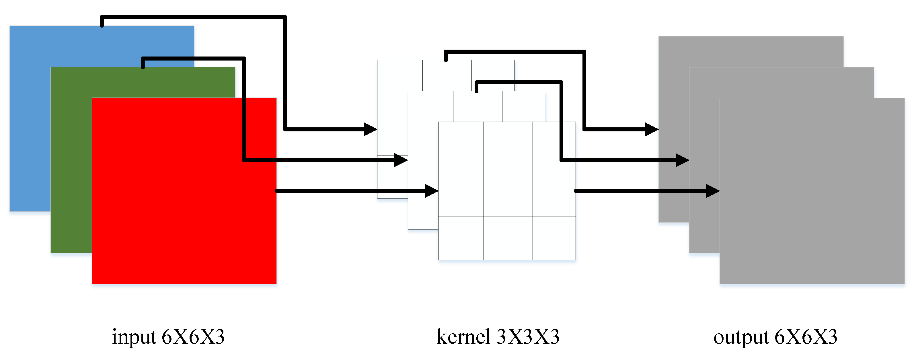
Depthwise separable convolution [22] includes a depthwise convolution and a pointwise convolution. When inputting a pixel, three-channel picture data (shape is 6 × 6 × 3), in the convolution operation, use a convolution kernel; Padding = 1, Stride = 1. After the convolution operation was completed, there were three feature images, with a feature size of , as shown in Figure 4. The convolution kernel shape in this case is:
is the width of the convolution kernel, is the height of the convolution kernel, and is the number of input channels.
One of the filters contains only a convolution kernel with a size of , and the number of parameters in the convolution part is calculated as shown in Equation (4):
The amount of calculation is as follows:
is the width of the input picture, and is the height of the input picture.
After depthwise convolution, the feature graph with the same number of input channels can be output, and each feature graph only represents the corresponding characteristics of one input channel, without merging other channel features. It cannot express the characteristic information of navigation in the same spatial position on different channels. In order to make the convolution network have more abstract expression ability, we need more channel feature graph representation, so we need pointwise convolution to combine these feature graphs into a new feature graph.
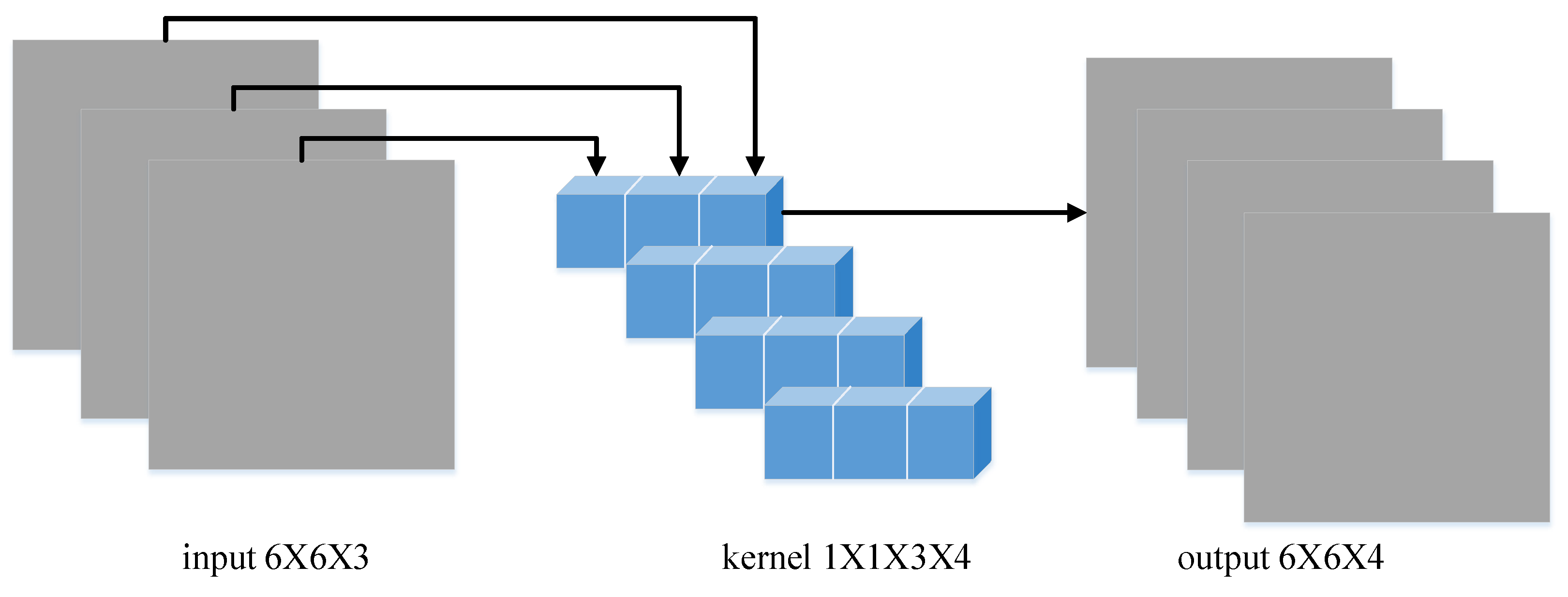
Pointwise convolution is a weighted combination of the characteristics of each input channel. The size of the convolution kernel used is . is the number of input channels in the point-by-point convolution layer. After pointwise convolution, a new feature graph is generated with characteristic information on the channel depth, as shown in Figure 5. The size of the convolution core of this layer is:
is the number of input channels, and is the number of output channels.
Because of the convolution operation of , the number of parameters involved in the point-by-point convolution is expressed as Equation (7):
The amount of calculation is as follows:
is the width of the input feature layer, and is the height of the input feature layer.
After pointwise convolution, four feature graphs are also output, which is the same as the output dimension of conventional convolution.
Compared with conventional convolution, the number of parameters is expressed:
The amount of calculation is as follows:
The comparison of the number of parameters and the amount of calculation with the conventional convolution algorithm is shown in Table 2:
As can be seen from Table 2 above, the number of parameters and the amount of computation of depthwise separable convolution are much smaller than that of the standard convolution operation. Therefore, the use of depthwise separable convolution can reduce the number of parameters generated by the convolution neural network in the process of model training while ensuring a certain accuracy, thus reducing the memory consumption of mobile devices and, on the other hand, reducing the amount of computation in the training phase of the model. A smaller amount of calculation correspondingly reduces the time required for model training.
3.2. Batch Normalization
In the process of convolution neural network training, batch normalization (BN) [23] makes the mean value of the output signal of this network layer 0, and the variance is 1. This operation can improve the decreasing speed of the loss value of the model and, at the same time, alleviate the “gradient dispersion” to a certain extent, and make the convolution network model converge more easily in the training stage. BN operations are generally used before nonlinear mapping functions.
3.3. Unpooling
Unpooling is the operation of increasing the image resolution and is the inverse operation of pooling, in which the position index information of the maximum value retained by the red operation is recorded during the max-pooling operation in the coding network part of the convolutional neural network, and the information is used to expand the feature graph when the max-unpooling operation is carried out in the decoding network. The specific operation is the maximum position of the maximum value. Except for the position of the maximum value, the rest is 0, as shown in Figure 6.
4. Convolution Neural Network Based on H-Swish Activation Function
The activation function layer uses the activation function to simulate the characteristics of human brain neurons, controls whether the neurons are in an excited state, increases the nonlinear characteristics of the convolution neural network, and increases the ability of the convolution neural network to express the abstract features in the image. The rectified liner unit (ReLU) function [24] is a piecewise function, which is defined as:
As shown in Figure 7, the gradient of the ReLU function is 1 when x≥0, and vice versa.
Because the convolution neural network constructed in this paper is aimed at the mobile end of the forklift AGV equipment and is limited by the computing power of the mobile end, it was considered in order to reduce the computational complexity of the model. Therefore, the H-Swish function was used instead of the ReLU function, which can not only improve the accuracy, but also reduce the computational pressure of the forklift AGV equipment to a certain extent. The Swish [25] function can optimize the effect of the deep convolution network model to a certain extent, which is defined as:
The Swish activation function has no upper bound or lower bound and is smooth and nonmonotonous. However, the calculation of the sigmoid function contained in the function is not friendly to forklift AGV equipment. The value of the H-Swish activation function is similar to that of the Swish activation function, and there is no sigmoid function operation in H-Swish, so it is friendly to the calculation of forklift AGV equipment. The definition is as follows:
5. Model Training and Analysis of Experimental Results
In order to realize the convolution neural network established in this paper, it was used to identify the road scene of forklift AGV equipment in a distribution center warehouse, using the PyTorch deep learning framework, which is the most popular in the field of deep learning and is very suitable for image data processing. We used the GPU computing model, which can improve the computing speed of the convolution neural network. The graphics card used in the model training was 6G NVIDIA GTX1660, video memory, and only one video card was used for training.
5.1. Data Preparation
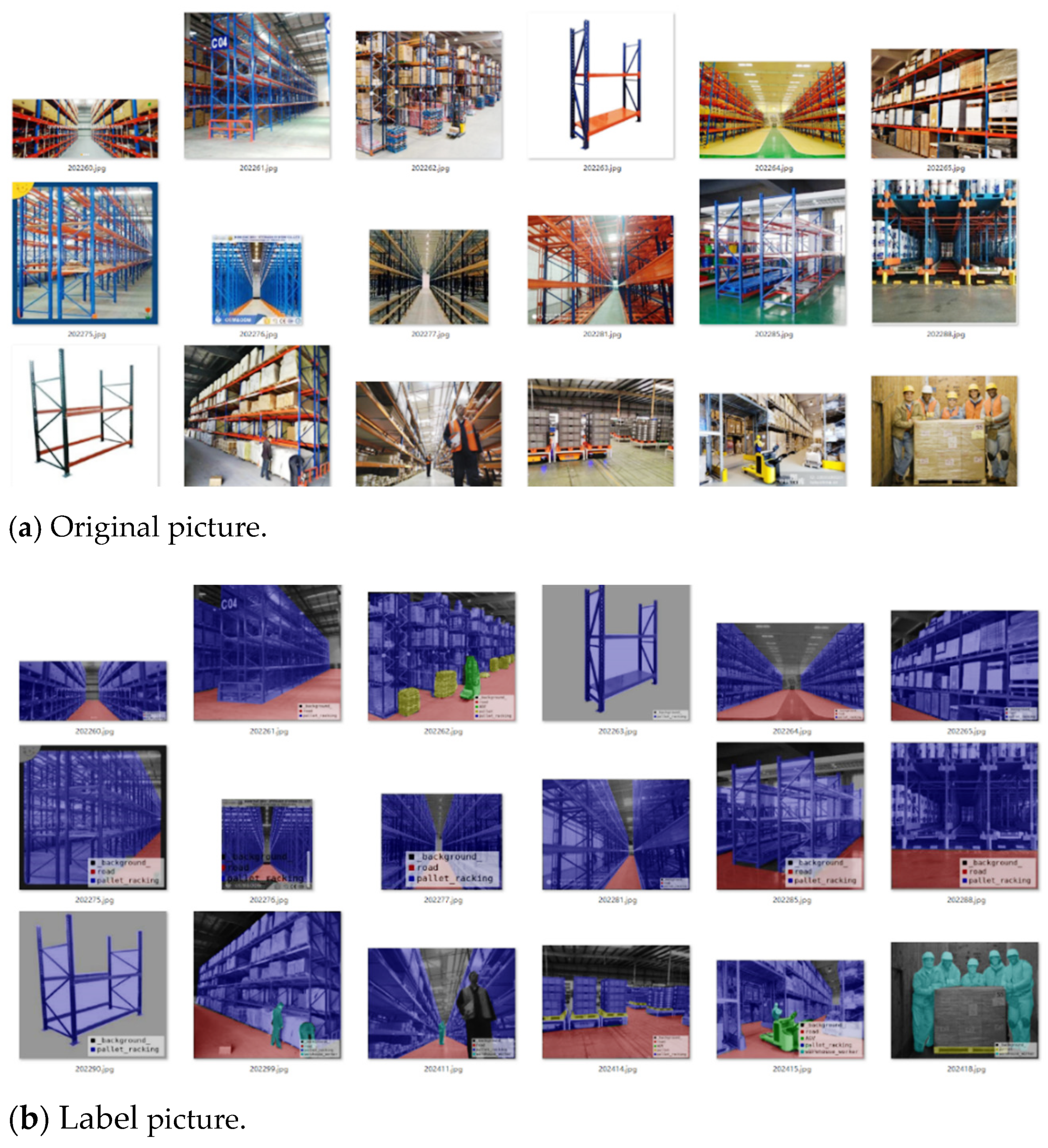
The convolution neural network established in this paper learns image features from label data, so it needs a distribution center environment image dataset with tags. We used the self-built dataset, including the warehouse environment picture dataset, including 469 logistics distribution center warehouse environment pictures, pictures from Google, Baidu, Bing, and other search engines. The dataset part is as shown in Figure 8. Because the training convolution neural network needs labeled label data, and the dataset built in this paper is only the original picture, we needed to label these pictures manually. The labeling tool was LABELME. In the dataset label, there are six types of tags: shelf, AGV car, pedestrian, ground, pallet, goods. Therefore, these six kinds of objects were segmented in the experiment.
5.2. Model Training
The self-built warehouse dataset of the logistics distribution center was used to train the convolution neural network. The dataset includes 375 color training pictures, with a resolution of 224 × 224 and 94 color training pictures, all of which are marked with information. When training the convolution neural network, the random batch processing (Mini-Batch) training mechanism was adopted, the training iteration number of the model was set to 3000, and the training sequence of pictures was randomly generated before each round of training to ensure that the pictures of each round of training were not the same. The generalization ability of the model was increased, and the convergence speed was improved. In the data processing of the convolution neural network, the resolution of the input picture was 224 × 224, but the resolution of the dataset was inconsistent. By compressing the picture, the resolution of the picture was unified to facilitate the input data of the neural network. The objective function of convolution neural network training was the cross-entropy loss function, the learning rate of network training was , the momentum parameter was 0.9, and every eight pictures were used as a batch of network input (limited by video memory; the larger the number of pictures in batches, the better the training effect).
5.3. Analysis of Experimental Results of Network Model Based on Depthwise Separable Convolution
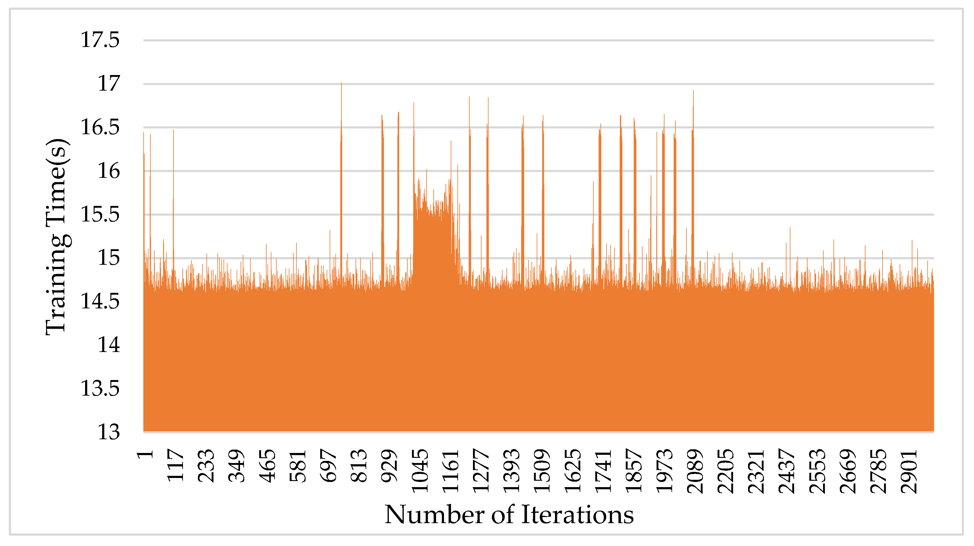
In order to compare the difference between the network model based on depthwise separable convolution and the original model, the same training set is used to train the model in the environment of the same hardware equipment. In this paper, 375 pictures were used for training and 94 pictures were used for testing. The experiment used six types of tags for training, with a batch size of eight. There were 3000 iterations and 64 epochs of training, and the time consumption in the training process is shown in Figure 9 and Figure 10.
Among them, batch size is the number of images selected in the dataset for training, usually 8, 16, 32. Iteration completes an iteration for the network model, training a batch-sized picture. Epochs is the number of times the training traverses the dataset. An epoch indicates that each image in the training set participates in the training once. In this experiment, there were 3000 iterations. If the batch size of the training set is eight, then the number of epochs is 64.
As shown in Figure 9, the average training time per round of the network model with depthwise separable convolution was 12.41 s, and the total training time was 10.34 h. In the traditional convolution operation network model, the average training time per round is 14.83 s, and the total training time is 12.36 h. It can be seen that the depthwise separable convolution has an obvious effect on reducing the training time of the model.
After 3000 iterations, both the depthwise separable convolution network model and the original model are basically in a state of convergence, and the loss value is reduced to 2.49. The experimental results show that, in the convolution network model with depthwise separable convolution, although the parameters of the model are reduced, the accuracy of the model is not affected, and the loss value is basically the same as that of the original model, which confirms the effectiveness of the application of depthwise separable convolution.
The number of network model parameters based on depthwise separable convolution is 27.94 million, as shown in Table 3, and the number of parameters of the original model is 29.43 million, which is 1.49 million, and 5% lower than that of the original model. The maximum number of pooled layer and soft connection layer parameters is 0.
5.4. Analysis of Network Model Experiment Results Based on H-Swish Activation Function
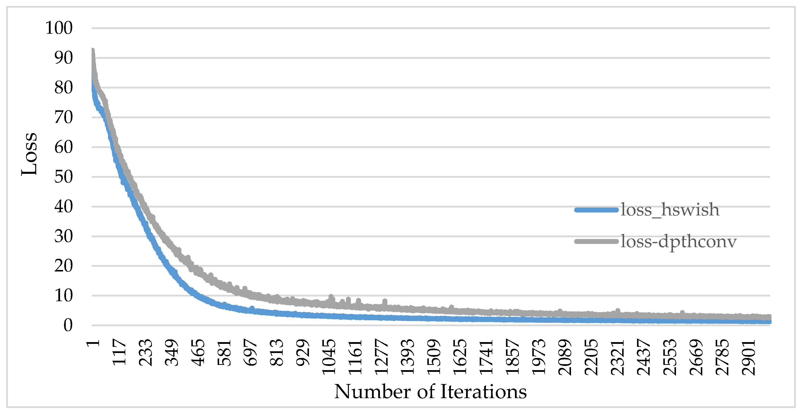
In order to compare the training results of the network model using the H-Swish activation function with that of the network model using the ReLU activation function, this paper used the same dataset to train the network model. The two models went through 3000 iterations each, and the loss value in the training process is shown in Figure 11 below:
As can be seen from Figure 11, the loss value (loss) of the H-Swish activation function is significantly lower than that of the ReLU activation function: the lowest loss value of the H-Swish activation function is 1.2, and the lowest loss value of using the ReLU activation function is 2.4. The comparison of the experimental data shows that the convolution network model using the H-Swish activation function has higher accuracy. In the convolution network model using the H-Swish activation function, the superiority of the activation function is proven. There is no sigmoid function operation in the activation function, so it is friendly to the calculation of forklift AGV equipment.
As shown in Figure 12, 3000 epochs were trained with the network model of the H-Swish activation function and the ReLU activation function, and the segmentation results on the test set image are shown. In the image semantic segmentation, the segmentation effect of using the H-Swish activation function is better, and the segmentation of the target analogy is smoother and more accurate. From the above experimental results, we can see that the segmentation effect of using the H-Swish activation function is better, indicating that using this activation function can improve the performance of the convolution neural network.
6. Conclusions
In this paper, the basic principle of depthwise separable convolution is described, and a neural network model based on depthwise separable convolution is proposed on the basis of the SegNet network model. Compared with the original model, the network model established in this chapter has a lower number of parameters and calculations, less memory consumption of the computing equipment in model training, and a shorter convergence time of the training model. On the premise of ensuring the accuracy of the model, the number of parameters of the model proposed in this paper is 1.49 million less than that of the traditional model, and the training time is saved by two hours. The model uses the H-Swish activation function to further improve the accuracy of the model on the basis of reducing the number of model parameters. When using the H-Swish function as the activation function, the loss value is lower than that of ReLU activation function. H-Swish has no sigmoid operation, which reduces the amount of model calculations and is more suitable for the operation of mobile devices, such as forklifts. The network model of this paper was trained by a self-built dataset, which included the data of all kinds of equipment in the logistics distribution center warehouse, which can provide reliable data for the neural network in order to better adapt to the working environment of the warehouse and make the model more suitable for the application of warehouse scene understanding.
This research does not take the small-label objects in the forklift operation environment into account. The classification label types can be improved to make the model suitable for the general industrial environment, which is also a direction for future research.
Author Contributions
Conceptualization, Y.W.; model building, R.Z.; methodology, G.L.; investigation, R.M.; resources, G.L.; experiment, R.Z.; supervision, G.L.; validation, R.M.; writing—original draft, Y.W.; writing—review and editing, R.M. All authors have read and agreed to the published version of the manuscript.
Funding
This research was funded by the Science, Technology and Innovation Commission of ShenZhen Municipality, grant number (No. JCYJ20190807094803721), and Shandong Provincial Natural Science Foundation, grant number (No. ZR2020MF085).
Institutional Review Board Statement
Not applicable.
Informed Consent Statement
Not applicable.
Acknowledgments
We thank other colleagues at the Modern Logistics Research Center of Shandong University for their help.
Conflicts of Interest
The authors declare no conflict of interest.
References
- Wu, H.; Chi, J.; Tian, G. Instance recognition and semantic mapping based on visual SLAM. J. Huazhong Univ. Sci. Tech. Nat. Sci. Ed. 2019, 47, 48–54. [Google Scholar]
- Wang, M.; Han, B.; Luo, Q. Binocular Visual Navigation and Obstacle Avoidance of Mobile Robots Based on Speeded-Up Robust Features. CADDM 2013, 4, 18–24. [Google Scholar]
- Long, J.; Shelhamer, E.; Darrell, T. Fully Convolutional Networks for Semantic Segmentation. IEEE Trans. Pattern Anal. Mach. Intell. 2015, 39, 640–651. [Google Scholar]
- Noh, H.; Hong, S.; Han, B. Learning Deconvolution Network for Semantic Segmentation. In Proceedings of the IEEE International Conference on Computer Vision (ICCV), Santiago, Chile, 7–13 December 2015; pp. 1520–1528. [Google Scholar]
- Badrinarayanan, V.; Kendall, A.; Cipolla, R. SegNet: A Deep Convolutional Encoder-Decoder Architecture for Image Segmentation. IEEE Trans. Pattern Anal. Mach. Intell. 2017, 39, 2481–24951. [Google Scholar] [CrossRef] [PubMed]
- Lin, G.; Milan, A.; Shen, C.; Reid, I. RefineNet: Multi-Path Refinement Networks for High-Resolution Semantic Segmentation. In Proceedings of the 30th IEEE Conference on Computer Vision and Pattern Recognition, Honolulu, HI, USA, 21–26 July 2017; pp. 5168–5177. [Google Scholar] [CrossRef] [Green Version]
- Liu, Z. Research of A Local Planner Based on Stereo and 2D Lidar. Master’s Thesis, University of Electronic Science and Technology of China, Chengdu, China, 2019. [Google Scholar]
- Zhang, X.; Gao, H.; Zhao, J.; Zhou, M. Overview of deep learning intelligent driving method. J. Tsinghua Univ. Sci. Technol. 2018, 58, 438–444. [Google Scholar]
- Mur-Artal, R.; Tardos, J.D. ORB-SLAM2: An opensource slam system for monocular, stereo, and RGB-D cameras. IEEE Trans. Robot. 2017, 33, 1–8. [Google Scholar] [CrossRef] [Green Version]
- Fang, L.; Liu, B.; Wan, Y. Semantic SLAM based on deep learning in dynamic scenes. J. Huazhong Univ. Sci. Tech. Nat. Sci. Ed. 2020, 48, 121–126. [Google Scholar]
- Simonyan, K.; Zisserman, A. Very Deep Convolutional Networks for Large-Scale Image Recognition. In Proceedings of the 3rd International Conference on Learning Representations, ICLR 2015, San Diego, CA, USA, 7–9 May 2015. [Google Scholar]
- Chen, L.C.; Papandreou, G.; Kokkinos, I.; Murphy, K.; Yuille, A. DeepLab: Semantic Image Segmentation with Deep Convolutional Nets, Atrous Convolution, and Fully Connected CRFs. IEEE Trans. Pattern Anal. Mach. Intell. 2018, 40, 834–848. [Google Scholar] [CrossRef] [PubMed]
- Chen, C.; Tang, S.; Li, J. Weakly supervised semantic segmentation based on dynamic mask generation. J. Image Graph. 2020, 25, 1190–1200. [Google Scholar]
- Souly, N.; Spampinato, C.; Shah, M. Semi supervised semantic segmentation using generative adversarial network. In Proceedings of the IEEE International Conference on Computer Vision (ICCV), Venice, Italy, 22–29 October 2017; pp. 5689–5697. [Google Scholar]
- Wei, Y.; Feng, J.; Liang, X.; Cheng, M.; Zhao, Y.; Yan, S. Object region mining with adversarial erasing: A simple classification to semantic segmentation approach. In Proceedings of the IEEE Conference on Computer Vision and Pattern Recognition, College Park, MD, USA, 25–26 February 2017; pp. 1568–1576. [Google Scholar]
- Zhang, X.; Wei, Y.; Feng, J.; Yang, Y.; Huang, T. Adversarial complementary learning for weakly supervised object localization. In Proceedings of the IEEE Computer Society Conference on Computer Vision and Pattern Recognition, Salt Lake City, UT, USA, 18–23 June 2018; pp. 1325–1334. [Google Scholar]
- Courbariaux, M.; Bengio, Y.; David, J.P. BinaryConnect: Training Deep Neural Networks with binary weights during propagations. In Proceedings of the Advances in Neural Information Processing Systems, Convention Center, Montreal, QC, Canada, 7–12 December 2015; pp. 3123–3131. [Google Scholar]
- Prewitt, J.; Mendelsohn, M.L. The analysis of cell images. Ann. N. Y. Acad. Sci. 1966, 128, 1035–1053. [Google Scholar] [CrossRef] [PubMed]
- Fukunaga, K.; Hostetler, L. The estimation of the gradient of a density function, with applications in pattern recognition. IEEE Trans. Inf. Theory 2006, 21, 32–40. [Google Scholar] [CrossRef] [Green Version]
- Bai, X.; Wang, W. Saliency-SVM: An automatic approach for image segmentation. Neurocomputing 2014, 136, 243–255. [Google Scholar] [CrossRef]
- Chen, L.C.; Papandreou, G.; Kokkinos, I.; Murphy, K.; Yuille, A.L. Semantic Image Segmentation with Deep Convolutional Nets and Fully Connected CRFs. In Proceedings of the 3rd International Conference on Learning Representations, ICLR 2015, San Diego, CA, USA, 7–9 May 2015. [Google Scholar]
- Sandler, M.; Howard, A.; Zhu, M.; Zhmoginov, A.; Chen, L.C. MobileNetV2: Inverted Residuals and Linear Bottlenecks. In Proceedings of the IEEE Computer Society Conference on Computer Vision and Pattern Recognition, Salt Lake City, UT, USA, 18–23 June 2018; pp. 4510–4520. [Google Scholar]
- Ioffe, S.; Szegedy, C. Batch Normalization: Accelerating Deep Network Training by Reducing Internal Covariate Shift. In Proceedings of the 32nd International Conference on Machine Learning, ICML, Lile, France, 6–11 July 2015; Batch, F., Blei, D., Eds.; pp. 448–456. [Google Scholar]
- Nair, V.; Hinton, G.E. Rectified Linear Units Improve Restricted Boltzmann Machines Vinod Nair. In Proceedings of the 27th International Conference on Machine Learning, Haifa, Israel, 21–24 June 2010; pp. 807–814. [Google Scholar]
- Ramachandran, P.; Zoph, B.; Le, Q.V. Searching for Activation Functions. In Proceedings of the 6th International Conference on Learning Representations, Vancouver, BC, Canada, 30 April–3 May 2018. [Google Scholar]
Figure 1.
Forklift AGV.

Figure 2.
Image semantic segmentation.

Figure 3.
The structure of the SegNet network.

Figure 4.
Depthwise convolution.

Figure 5.
Pointwise convolution.

Figure 6.
Unpooling.

Figure 7.
ReLU function and gradient.

Figure 8.
Distribution center environment image dataset.

Figure 9.
Model training time based on depthwise separable convolution.

Figure 10.
Model training time based on original model.

Figure 11.
H-Swish and ReLU activation function loss curve.

Figure 12.
Semantic segmentation results of ReLU and H-Swish activation functions.


Table 1.
Neural network model parameters based on depthwise separable convolution.
| Name | Type | Input Size | Parameters | Name | Type | Input Size | Parameters |
|---|---|---|---|---|---|---|---|
| Conv_00 | Convolution | 224*224 | 64,3*3,1,1 | Convtr_42d | Deconvolution | 14*14 | 512,3*3,1,1 |
| X_0 | Max pooling | 224*224 | 2*2,2 | Convtr_41d | Deconvolution | 14*14 | 512,3*3,1,1 |
| Conv_10 | Convolution | 112*112 | 64,3*3,1,1 | Convtr_40d | Deconvolution | 14*14 | 512,3*3,1,1 |
| Conv_11 | Convolution | 112*112 | 128,1*1,0,1 | X_3d | Max Unpooling | 14*14 | 2*2,2 |
| X_1 | Max Pooling | 112*112 | 2*2,2 | Convtr_32d | Deconvolution | 28*28 | 512,3*3,1,1 |
| Conv_20 | Convolution | 56*56 | 128,3*3,1,1 | Convtr_31d | Deconvolution | 28*28 | 512,3*3,1,1 |
| Conv_21 | Convolution | 56*56 | 256,1*1,0,1 | Convtr_30d | Deconvolution | 28*28 | 256,3*3,1,1 |
| Conv_22 | Convolution | 56*56 | 256,3*3,1,1 | X_2d | Max Unpooling | 28*28 | 2*2,2 |
| X_2 | Max Pooling | 56*56 | 2*2,2 | Convtr_22d | Deconvolution | 56*56 | 256,3*3,1,1 |
| Conv_30 | Convolution | 28*28 | 256,3*3,1,1 | Convtr_21d | Deconvolution | 56*56 | 256,3*3,1,1 |
| Conv_31 | Convolution | 28*28 | 512,1*1,0,1 | Convtr_20d | Deconvolution | 56*56 | 128,3*3,1,1 |
| Conv_32 | Convolution | 28*28 | 512,3*3,1,1 | X_1d | Max Unpooling | 56*56 | 2*2,2 |
| Conv_33 | Convolution | 28*28 | 512,3*3,1,1 | Convtr_11d | Deconvolution | 112*112 | 128,3*3,1,1 |
| X_3 | Max Pooling | 28*28 | 2*2,2 | Convtr_10d | Deconvolution | 112*112 | 64,3*3,1,1 |
| Conv_40 | Convolution | 14*14 | 512,3*3,1,1 | X_0d | Max Unpooling | 112*112 | 2*2,2 |
| Conv_41 | Convolution | 14*14 | 512,3*3,1,1 | Convtr_01d | Deconvolution | 224*224 | 64,3*3,1,1 |
| Conv_42 | Convolution | 14*14 | 512,3*3,1,1 | Convtr_01d | Deconvolution | 224*224 | 8,3*3,1,1 |
| X_4 | Max Pooling | 14*14 | 2*2,2 | Softmax | |||
| X_4d | Max Unpooling | 7*7 | 2*2,2 |
Note: The input size represents the input feature pixel. The parameters of convolution (Conv_*) and deconvolution (Convtr_*) are separated by commas, which, in turn, represent the number of output channels, the convolution kernel size, and the padding and stride. The parameters of max-pooling and max-unpooling are the pooling window size and step size, respectively.
Table 2.
Comparison between depthwise separable convolution and conventional convolution.
| Amount of Calculation | Number of Parameters |
|---|---|
Table 3.
Network model parameter scale based on depthwise separable convolution.
| Name | Input Size | Parameters | Number | Name | Input Size | Parameters | Number |
|---|---|---|---|---|---|---|---|
| Conv_00 | 224*224 | 64,3*3,1,1 | 1792 | Convtr_41d | 14*14 | 512,3*3,1,1 | 2359808 |
| Conv_10 | 112*112 | 64,3*3,1,1 | 36928 | Convtr_40d | 14*14 | 512,3*3,1,1 | 2359808 |
| Conv_11 | 112*112 | 128,1*1,0,1 | 8320 | Convtr_32d | 28*28 | 512,3*3,1,1 | 2359808 |
| Conv_20 | 56*56 | 128,3*3,1,1 | 147584 | Convtr_31d | 28*28 | 512,3*3,1,1 | 2359808 |
| Conv_21 | 56*56 | 256,1*1,0,1 | 33024 | Convtr_30d | 28*28 | 256,3*3,1,1 | 1180160 |
| Conv_22 | 56*56 | 256,3*3,1,1 | 590080 | Convtr_22d | 56*56 | 256,3*3,1,1 | 590080 |
| Conv_30 | 28*28 | 256,3*3,1,1 | 590080 | Convtr_21d | 56*56 | 256,3*3,1,1 | 590080 |
| Conv_31 | 28*28 | 512,1*1,0,1 | 13312 | Convtr_20d | 56*56 | 128,3*3,1,1 | 295168 |
| Conv_32 | 28*28 | 512,3*3,1,1 | 2359808 | Convtr_11d | 112*112 | 128,3*3,1,1 | 147584 |
| Conv_33 | 28*28 | 512,3*3,1,1 | 2359808 | Convtr_10d | 112*112 | 64,3*3,1,1 | 73856 |
| Conv_40 | 14*14 | 512,3*3,1,1 | 2359808 | Convtr_01d | 224*224 | 64,3*3,1,1 | 36828 |
| Conv_41 | 14*14 | 512,3*3,1,1 | 2359808 | Convtr_01d | 224*224 | 8,3*3,1,1 | 4608 |
| Conv_42 | 14*14 | 512,3*3,1,1 | 2359808 | Total | 27937564 | ||
| Convtr_42d | 14*14 | 512,3*3,1,1 | 2359808 |
Publisher’s Note: MDPI stays neutral with regard to jurisdictional claims in published maps and institutional affiliations. |
© 2021 by the authors. Licensee MDPI, Basel, Switzerland. This article is an open access article distributed under the terms and conditions of the Creative Commons Attribution (CC BY) license (https://creativecommons.org/licenses/by/4.0/).
Share and Cite
MDPI and ACS Style
Liu, G.; Zhang, R.; Wang, Y.; Man, R. Road Scene Recognition of Forklift AGV Equipment Based on Deep Learning. Processes 2021, 9, 1955. https://doi.org/10.3390/pr9111955
AMA Style
Liu G, Zhang R, Wang Y, Man R. Road Scene Recognition of Forklift AGV Equipment Based on Deep Learning. Processes. 2021; 9(11):1955. https://doi.org/10.3390/pr9111955
Chicago/Turabian StyleLiu, Gang, Rongxu Zhang, Yanyan Wang, and Rongjun Man. 2021. "Road Scene Recognition of Forklift AGV Equipment Based on Deep Learning" Processes 9, no. 11: 1955. https://doi.org/10.3390/pr9111955
Note that from the first issue of 2016, this journal uses article numbers instead of page numbers. See further details here.