
Validation of Novel Lattice Boltzmann Large Eddy Simulations (LB LES) for Equipment Characterization in Biopharma

 , ,
, ,  and
and 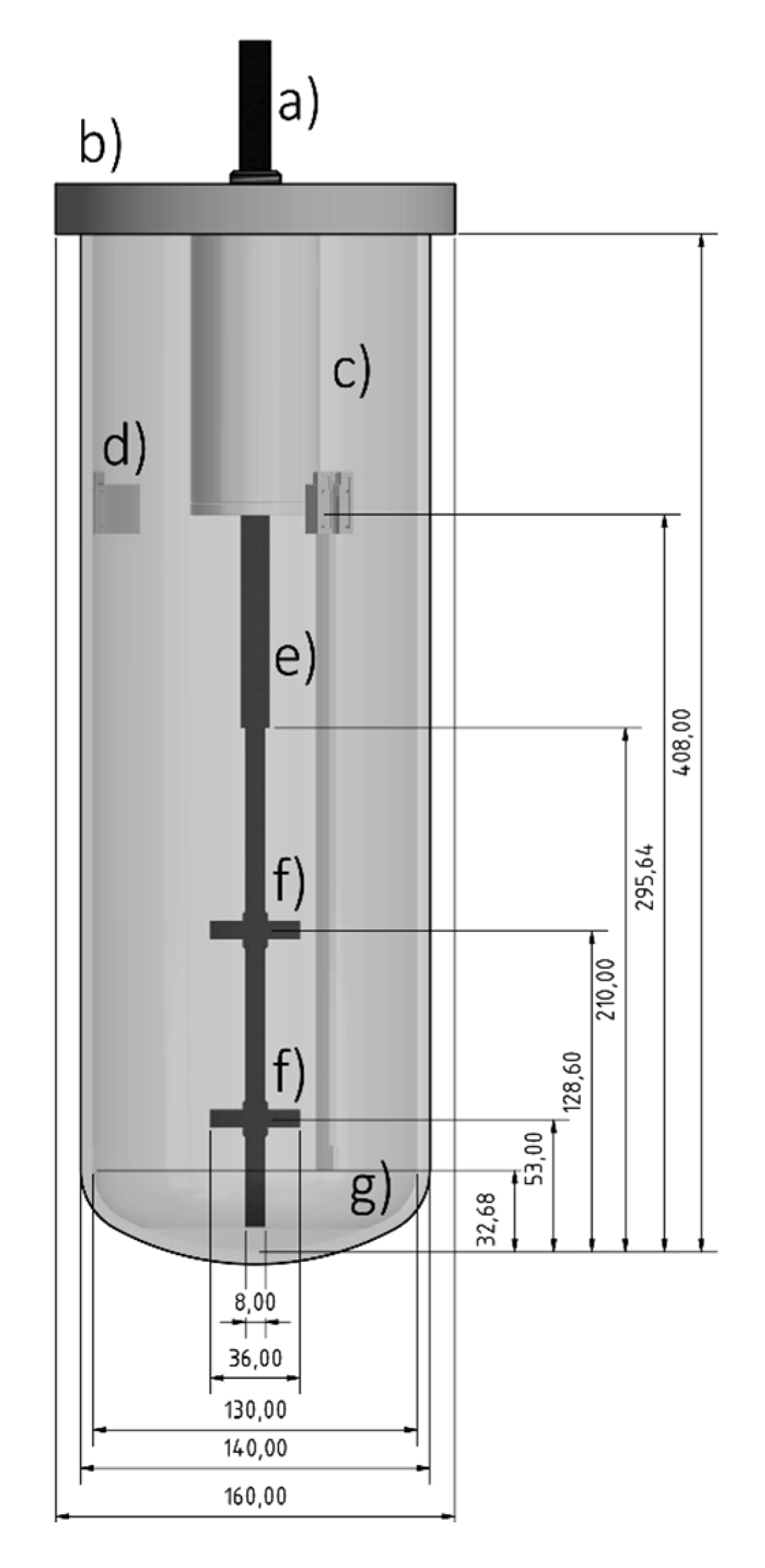
Abstract
1. Introduction
2. Materials and Methods
2.1. Reactor Setup
2.2. Experimental Setup
2.3. Numerical Simulations
3. Results and Discussion
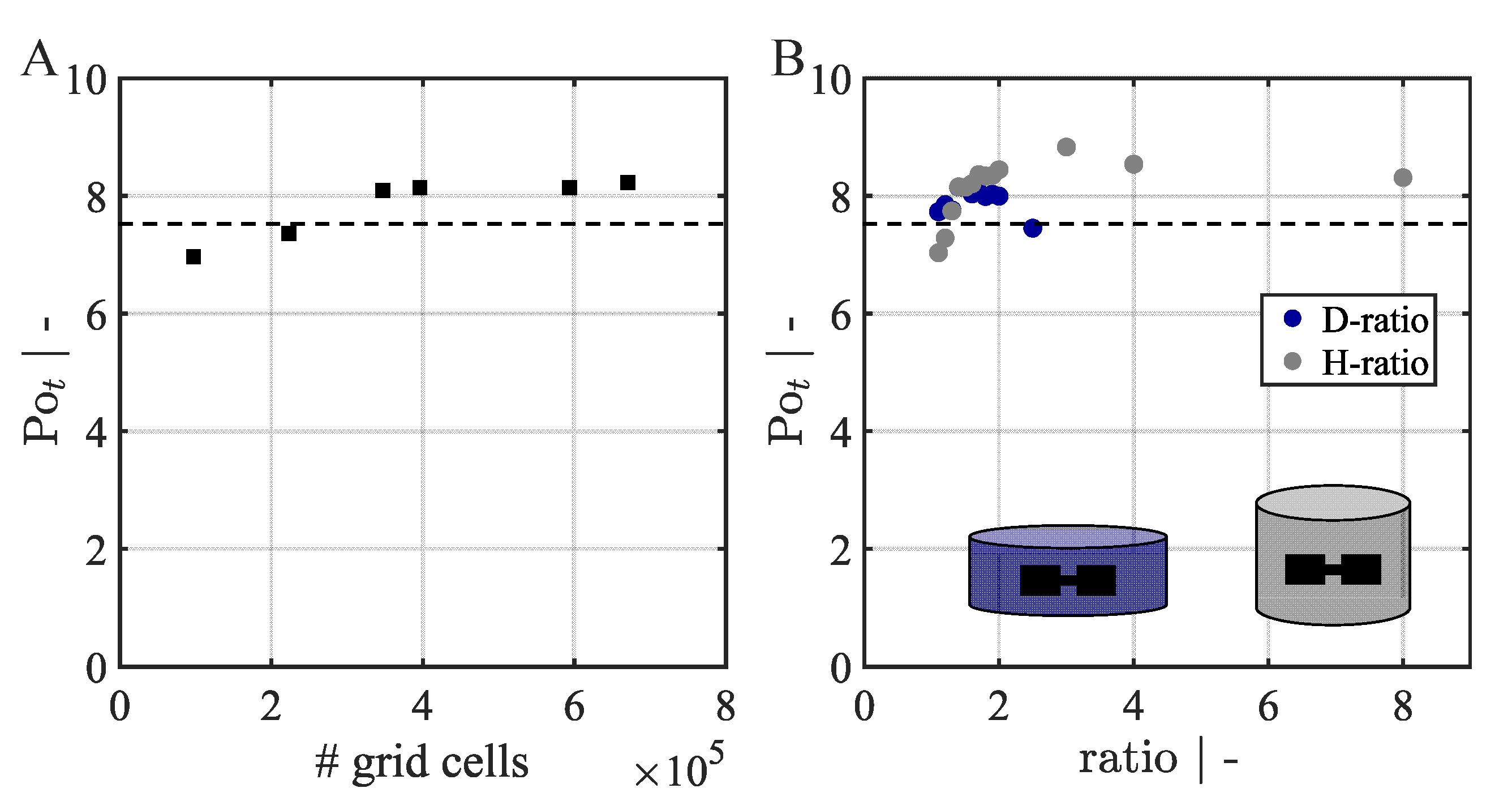
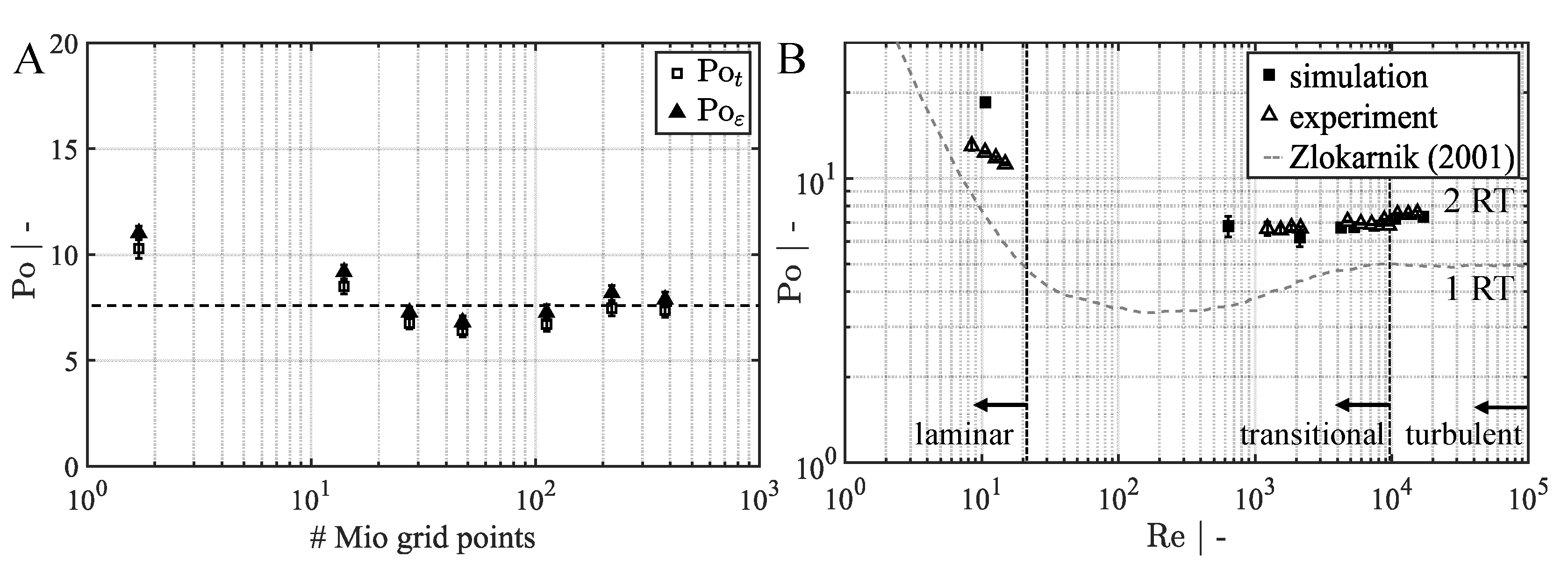
3.1. Steady State Simulations
3.2. Transient Simulations
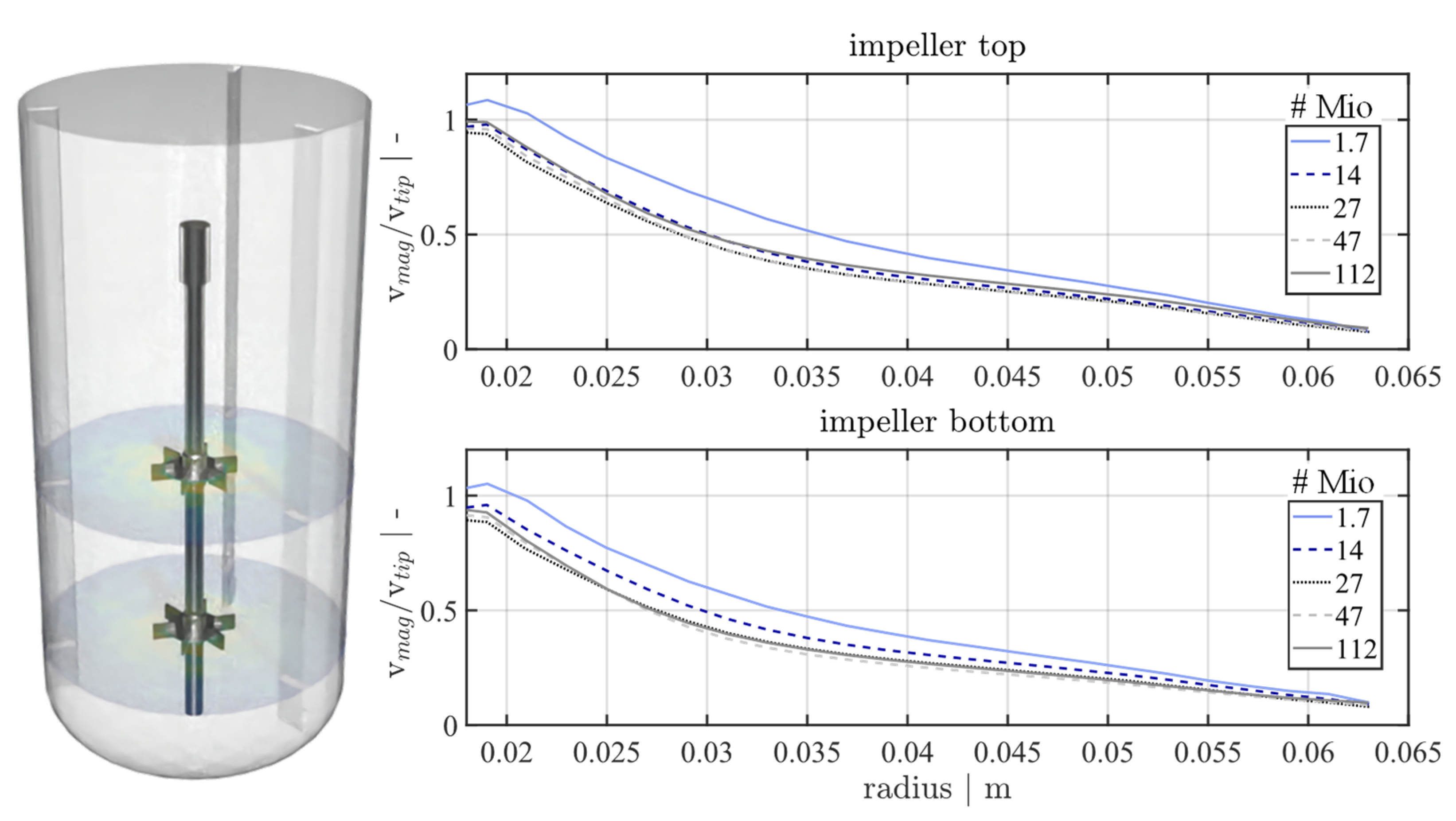
3.2.1. Grid Refinement Study
3.2.2. Validation of Numerical Simulations by 4D PTV Data
4. Conclusions
Supplementary Materials
Author Contributions
Funding
Institutional Review Board Statement
Informed Consent Statement
Data Availability Statement
Acknowledgments
Conflicts of Interest
Abbreviation
| Latin | Greek | |||
| Off-bottom clearance, m | Impeller spacing, m | |||
| Courant number | Time step, s | |||
| Impeller diameter, m | Grid spacing, m | |||
| Tank diameter, m | Dynamic viscosity, Pa s | |||
| Probability density function | Density, kg m−3 | |||
| Gravitational acceleration, m s−2 | Collision operator | |||
| Tank height, m | Energy dissipation rate, m2 s−3 | |||
| Surface height, m | Surface tension, N m−1 | |||
| Torque, N m | ||||
| Agitation rate, rpm | ||||
| Pressure, Pa | ||||
| Power, W m−3 | ||||
| 0 | Power number | |||
| Power by torque, W | ||||
| Power by energy dissipation, W | ||||
| r | Radial distance, m | |||
| Re | Reynolds number | |||
| Spatial resolution, m | ||||
| Time, s | ||||
| Three-dimensional velocity vector, m s−1 | ||||
| Tip speed, m s−1 | ||||
| Velocity magnitude, m s−1 | ||||
| Volume, m3 |
References
- Wutz, J.; Steiner, R.; Assfalg, K.; Wucherpfennig, T. Establishment of a CFD-Based kLa Model in Microtiter Plates to Support CHO Cell Culture Scale-up during Clone Selection. Biotechnol. Prog. 2018, 34, 1120–1128. [Google Scholar] [CrossRef]
- Wutz, J.; Waterkotte, B.; Heitmann, K.; Wucherpfennig, T. Computational Fluid Dynamics (CFD) as a Tool for Industrial UF/DF Tank Optimization. Biochem. Eng. J. 2020, 160, 107617. [Google Scholar] [CrossRef]
- Waghmare, Y.; Falk, R.; Graham, L.; Koganti, V. Drawdown of Floating Solids in Stirred Tanks: Scale-up Study Using CFD Modeling. Int. J. Pharm. 2011, 418, 243–253. [Google Scholar] [CrossRef]
- Roush, D.; Asthagiri, D.; Babi, D.K.; Benner, S.; Bilodeau, C.; Carta, G.; Ernst, P.; Fedesco, M.; Fitzgibbon, S.; Flamm, M.; et al. Toward in Silico CMC: An Industrial Collaborative Approach to Model-Based Process Development. Biotechnol. Bioeng. 2020, 117, 3986–4000. [Google Scholar] [CrossRef]
- Falk, R.F.; Marziano, I.; Kougoulos, T.; Girard, K.P. Prediction of Agglomerate Type during Scale-Up of a Batch Crystallization Using Computational Fluid Dynamics Models. Org. Process. Res. Dev. 2011, 15, 1297–1304. [Google Scholar] [CrossRef]
- Ladner, T.; Odenwald, S.; Kerls, K.; Zieres, G.; Boillon, A.; Boeuf, J. CFD Supported Investigation of Shear Induced by Bottom-Mounted Magnetic Stirrer in Monoclonal Antibody Formulation. Pharm. Res. 2018, 35, 215. [Google Scholar] [CrossRef] [PubMed]
- Saleh, D.; Wang, G.; Muller, B.; Rischawy, F.; Kluters, S.; Studts, J.; Hubbuch, J. Straightforward Method for Calibration of Mechanistic Cation Exchange Chromatography Models for Industrial Applications. Biotechnol. Prog. 2020, 36, e2984. [Google Scholar] [CrossRef] [PubMed]
- Narayanan, H.; Luna, M.F.; Stosch, M.v.; Bournazou, M.N.C.; Polotti, G.; Morbidelli, M.; Butte, A.; Sokolov, M. Bioprocessing in the Digital Age: The Role of Process Models. Biotechnol. J. 2020, 15, e1900172. [Google Scholar] [CrossRef]
- Smiatek, J.; Jung, A.; Bluhmki, E. Towards a Digital Bioprocess Replica: Computational Approaches in Biopharmaceutical Development and Manufacturing. Trends Biotechnol. 2020, 38, 1141–1153. [Google Scholar] [CrossRef]
- Bakker, A.; Oshinowo, L.M. Modelling of Turbulence in Stirred Vessels Using Large Eddy Simulation. Chem. Eng. Res. Des. 2004, 82, 1169–1178. [Google Scholar] [CrossRef]
- Delafosse, A.; Line, A.; Morchain, J.; Guiraud, P. LES and URANS Simulations of Hydrodynamics in Mixing Tank: Comparison to PIV Experiments. Chem. Eng. Res. Des. 2008, 86, 1322–1330. [Google Scholar] [CrossRef]
- Hartmann, H.; Derksen, J.J.; Montavon, C.; Pearson, J.; Hamill, I.S.; Akker, H.E.A. van den Assessment of Large Eddy and RANS Stirred Tank Simulations by Means of LDA. Chem. Eng. Sci. 2004, 59, 2419–2432. [Google Scholar] [CrossRef]
- Jahoda, M.; Mostĕk, M.; Kukukova, A.; Machon, V. CFD Modelling of Liquid Homogenization in Stirred Tanks with One and Two Impellers Using Large Eddy Simulation. Chem. Eng. Res. Des. 2007, 85, 616–625. [Google Scholar] [CrossRef]
- Guidance for Industry and Food and Drug Administration Staff. Reporting of Computational Modeling Studies in Medical Device Submissions, FDA-2013-D-1530; Department of Health and Human Services: Washington, DC, USA, 2016. [Google Scholar]
- Sieblist, C.; Hägeholz, O.; Aehle, M.; Jenzsch, M.; Pohlscheidt, M.; Lübbert, A. Insights into Large-scale Cell-culture Reactors: II. Gas-phase Mixing and CO2 Stripping. Biotechnol. J. 2011, 6, 1547–1556. [Google Scholar] [CrossRef] [PubMed]
- Coroneo, M.; Montante, G.; Paglianti, A.; Magelli, F. CFD Prediction of Fluid Flow and Mixing in Stirred Tanks: Numerical Issues about the RANS Simulations. Comput. Chem. Eng. 2011, 35, 1959–1968. [Google Scholar] [CrossRef]
- Ebrahimi, M.; Tamer, M.; Villegas, R.M.; Chiappetta, A.; Ein-Mozaffari, F. Application of CFD to Analyze the Hydrodynamic Behaviour of a Bioreactor with a Double Impeller. Process 2019, 7, 694. [Google Scholar] [CrossRef]
- Cortada-Garcia, M.; Dore, V.; Mazzei, L.; Angeli, P. Experimental and CFD Studies of Power Consumption in the Agitation of Highly Viscous Shear Thinning Fluids. Chem. Eng. Res. Des. 2017, 119, 171–182. [Google Scholar] [CrossRef]
- Murthy, B.N.; Joshi, J.B. Assessment of Standard k-ε, RSM and LES Turbulence Models in a Baffled Stirred Vessel Agitated by Various Impeller Designs. Chem. Eng. Sci. 2008, 63, 5468–5495. [Google Scholar] [CrossRef]
- Brucato, A.; Ciofalo, M.; Grisafi, F.; Micale, G. Numerical Prediction of Flow Fields in Baffled Stirred Vessels: A Comparison of Alternative Modelling Approaches. Chem. Eng. Sci. 1998, 53, 3653–3684. [Google Scholar] [CrossRef]
- Jaszczur, M.; Mynarczykowska, A. A General Review of the Current Development of Mechanically Agitated Vessels. Process 2020, 8, 982. [Google Scholar] [CrossRef]
- Zadravec, M.; Basic, S.; Hribersek, M. The Influence of Rotating Domain Size in a Rotating Frame of Reference Approach for Simulation of Rotating Impeller in a Mixing Vessel. J. Eng. Sci. Technol. 2007, 2, 126–138. [Google Scholar]
- Bach, C.; Yang, J.; Larsson, H.; Stocks, S.M.; Gernaey, K.V.; Albaek, M.O.; Kruhne, U. Evaluation of Mixing and Mass Transfer in a Stirred Pilot Scale Bioreactor Utilizing CFD. Chem. Eng. Sci. 2017, 171, 19–26. [Google Scholar] [CrossRef]
- Haringa, C.; Vandewijer, R.; Mudde, R.F. Inter-Compartment Interaction in Multi-Impeller Mixing: Part I. Experiments and Multiple Reference Frame CFD. Chem. Eng. Res. Des. 2018, 136, 870–885. [Google Scholar] [CrossRef]
- Haringa, C.; Vandewijer, R.; Mudde, R.F. Inter-Compartment Interaction in Multi-Impeller Mixing. Part II. Experiments, Sliding Mesh and Large Eddy Simulations. Chem. Eng. Res. Des. 2018, 136, 886–899. [Google Scholar] [CrossRef]
- Witz, C.; Treffer, D.; Hardiman, T.; Khinast, J. Local Gas Holdup Simulation and Validation of Industrial-Scale Aerated Bioreactors. Chem. Eng. Sci. 2016, 152, 636–648. [Google Scholar] [CrossRef]
- Thomas, J.A.; Liu, X.; De Vincentis, B.; Hua, H.; Yao, G.; Borys, M.C.; Aron, K.; Pendse, G. A Mechanistic Approach for Predicting Mass Transfer in Bioreactors. Chem. Eng. Sci. 2021, 237, 116538. [Google Scholar] [CrossRef]
- Taghavi, M.; Zadghaffari, R.; Moghaddas, J.; Moghaddas, Y. Experimental and CFD Investigation of Power Consumption in a Dual Rushton Turbine Stirred Tank. Chem. Eng. Res. Des. 2011, 89, 280–290. [Google Scholar] [CrossRef]
- Thomas, J.; Sinha, K.; Shivkumar, G.; Cao, L.; Funck, M.; Shang, S.; Nere, N.K. A CFD Digital Twin to Understand Miscible Fluid Blending. AAPS PharmSciTech 2021, 22, 91. [Google Scholar] [CrossRef]
- Fitschen, J.; Hofmann, S.; Wutz, J.; Kameke, A.v.; Hoffmann, M.; Wucherpfennig, T.; Schluter, M. Novel Evaluation Method to Determine the Local Mixing Time Distribution in Stirred Tank Reactors. Chem. Eng. Sci. X 2021, 10, 100098. [Google Scholar] [CrossRef]
- Schanz, D.; Gesemann, S.; Schroder, A. Shake-The-Box: Lagrangian Particle Tracking at High Particle Image Densities. Exp. Fluids 2016, 57, 70. [Google Scholar] [CrossRef]
- Fitschen, J.; Maly, M.; Rosseburg, A.; Wutz, J.; Wucherpfennig, T.; Schluter, M. Influence of Spacing of Multiple Impellers on Power Input in an Industrial-Scale Aerated Stirred Tank Reactor. Chem. Ing. Tech. 2019, 91, 1794–1801. [Google Scholar] [CrossRef]
- Boussinesq, J. Theorie de L’ecoulement Tourbillant; Mem. De L’Acad. Des Sci: Paris, France, 1877; Volume 23. [Google Scholar]
- Succi, S. The Lattice Boltzmann Equation: For Fluid Dynamics and Beyond; Oxford University Press: Oxford, UK, 2001; ISBN 0198503989. [Google Scholar]
- Kruger, T.; Kusumaatmaja, H.; Kuzmin, A.; Shardt, O.; Silva, G.; Viggen, E.M. The Lattice Boltzmann Method; Springer: Basel, Switzerland, 2017. [Google Scholar]
- Mohamad, A.A. Lattice Boltzmann Method; Springer: Basel, Switzerland, 2011. [Google Scholar]
- Yu, H.; Girimaji, S.S.; Luo, L.-S. DNS and LES of Decaying Isotropic Turbulence with and without Frame Rotation Using Lattice Boltzmann Method. J. Comput. Phys. 2005, 209, 599–616. [Google Scholar] [CrossRef]
- Smagorinsky, J. General Circulation Experiments with the Primitive Equations: I. The Basic Experiment. Mon. Weather Rev. 1963, 91, 99–164. [Google Scholar] [CrossRef]
- Zhu, L.; He, G.; Wang, S.; Miller, L.; Zhang, X.; You, Q.; Fang, S. An Immersed Boundary Method Based on the Lattice Boltzmann Approach in Three Dimensions, with Application. Comput. Math. Appl. 2011, 61, 3506–3518. [Google Scholar] [CrossRef]
- Concha-Gomez, A.D.d.L.; Ramirez-Munoz, J.J.; Marquez-Banos, V.E.; Haro, C.; Alonso-Gomez, A.R. Effect of the Rotating Reference Frame Size for Simulating a Mixing Straight-Blade Impeller in a Baffled Stirred Tank. Rev. Mex. Ing. Química 2019, 18, 1143–1160. [Google Scholar] [CrossRef]
- Sommerfeld, M.; Decker, S. State of the Art and Future Trends in CFD Simulation of Stirred Vessel Hydrodynamics. Chem. Eng. Technol. 2004, 27, 215–224. [Google Scholar] [CrossRef]
- Lane, G.L.; Schwarz, M.P.; Evans, G.M. Chapter 34-Comparison of CFD Methods for Modelling of Stirred Tanks. In 10th European Conference on Mixing; Akker, H.E.A., van den Derksen, J.J., Eds.; Elsevier Science: Amsterdam, The Netherlands, 2000; ISBN 978-0-444-50476-0. [Google Scholar]
- Zlokarnik Stirrer Power. Stirring; Wiley-VCH: Weinheim, Germany, 2001. [Google Scholar]
- Nienow, A.; Wisdom, D. Flow over Disc Turbine Blades. Chem. Eng. Sci. 1974, 29, 1994–1997. [Google Scholar] [CrossRef]
- Riet, K.V.; Smith, J.M. The Trailing Vortex System Produced by Rushton Turbine Agitators. Chem. Eng. Sci. 1975, 30, 1093–1105. [Google Scholar]


Publisher’s Note: MDPI stays neutral with regard to jurisdictional claims in published maps and institutional affiliations. |
© 2021 by the authors. Licensee MDPI, Basel, Switzerland. This article is an open access article distributed under the terms and conditions of the Creative Commons Attribution (CC BY) license (https://creativecommons.org/licenses/by/4.0/).
Share and Cite
Kuschel, M.; Fitschen, J.; Hoffmann, M.; von Kameke, A.; Schlüter, M.; Wucherpfennig, T. Validation of Novel Lattice Boltzmann Large Eddy Simulations (LB LES) for Equipment Characterization in Biopharma. Processes 2021, 9, 950. https://doi.org/10.3390/pr9060950
Kuschel M, Fitschen J, Hoffmann M, von Kameke A, Schlüter M, Wucherpfennig T. Validation of Novel Lattice Boltzmann Large Eddy Simulations (LB LES) for Equipment Characterization in Biopharma. Processes. 2021; 9(6):950. https://doi.org/10.3390/pr9060950
Chicago/Turabian StyleKuschel, Maike, Jürgen Fitschen, Marko Hoffmann, Alexandra von Kameke, Michael Schlüter, and Thomas Wucherpfennig. 2021. "Validation of Novel Lattice Boltzmann Large Eddy Simulations (LB LES) for Equipment Characterization in Biopharma" Processes 9, no. 6: 950. https://doi.org/10.3390/pr9060950
APA StyleKuschel, M., Fitschen, J., Hoffmann, M., von Kameke, A., Schlüter, M., & Wucherpfennig, T. (2021). Validation of Novel Lattice Boltzmann Large Eddy Simulations (LB LES) for Equipment Characterization in Biopharma. Processes, 9(6), 950. https://doi.org/10.3390/pr9060950