
Higher Order Accurate Transient Numerical Model to Evaluate the Natural Convection Heat Transfer in Flat Plate Solar Collector


1
Building Energy Efficiency Group, CSIR-Central Building Research Institute, Roorkee 247667, India
2
Academy of Scientific and Innovative Research (AcSIR), Ghaziabad 201002, India
3
Department of Mechanical & Industrial Engineering, Indian Institute of Technology, Roorkee 247667, India
4
Faculty of Engineering, University of Rijeka, 51000 Rijeka, Croatia
*
Authors to whom correspondence should be addressed.
Processes 2021, 9(9), 1508; https://doi.org/10.3390/pr9091508
Submission received: 30 June 2021
/
Revised: 13 August 2021
/
Accepted: 20 August 2021
/
Published: 26 August 2021
(This article belongs to the Special Issue Enhancement of Heat Transfer and Fluid Flow)
Abstract
:The natural convection flow in the air gap between the absorber plate and glass cover of the flat plate solar collectors is predominantly evaluated based on the lumped capacitance method, which does not consider the spatial temperature gradients. With the recent advancements in the field of computational fluid dynamics, it became possible to study the natural convection heat transfer in the air gap of solar collectors with spatially resolved temperature gradients in the laminar regime. However, due to the relatively large temperature gradient in this air gap, the natural convection heat transfer lies in either the transitional regime or in the turbulent regime. This requires a very high grid density and a large convergence time for existing CFD methods. Higher order numerical methods are found to be effective for resolving turbulent flow phenomenon. Here we develop a non-dimensional transient numerical model for resolving the turbulent natural convection heat transfer in the air gap of a flat plate solar collector, which is fourth order accurate in both spatial and temporal domains. The developed model is validated against benchmark results available in the literature. An error of less than 5% is observed for the top heat loss coefficient parameter of the flat plate solar collector. Transient flow characteristics and various stages of natural convection flow development have been discussed. In addition, it was observed that the occurrence of flow mode transitions have a significant effect on the overall natural convection heat transfer.
1. Introduction
Solar collectors trap the solar radiation and convert it into thermal energy which has many applications, such as cooking, indoor space heating, hot water generation, distillation, steam production, solar air conditioning, etc. The conversion efficiency of solar energy into thermal energy at required temperatures should be as high as possible. This aspect requires understanding of the heat loss mechanism and various heat transfer mechanisms inside the solar collectors. All three heat transfer mechanisms, (conduction, convection and radiation), occur simultaneously inside the solar collector. The main heat losses in a Flat Plate Solar Collector (FPSC) are due to heat loss by convection in the air gap between the absorber plate and the glass cover of the FPSC, which constitutes approximately 70% of the total heat loss. The natural convection phenomenon inside this air gap lies in the turbulent regime due to a large temperature difference between the absorber plate and glass cover of an FPSC.
Several researchers have conducted experimental studies on solar collectors to optimize various design parameters to achieve maximum conversion efficiency while minimizing losses. Similarly, researchers have also developed analytical models to analyze the heat transfer phenomenon inside an FPSC. Duffie and Beckman [1] developed a steady state 1D model to evaluate the efficiency of an FPSC, which is a function of fluid temperature at the inlet. Nusselt number correlations have also been proposed to evaluate the heat transfer phenomenon inside the solar collector at a steady state. However, heat transfer during experiments lie mostly in the transient state since the incident solar radiation itself is continuously varying in nature. Therefore, the requirement of achieving steady state conditions during experiments to compare with the analytical results is impractical and uneconomical. Heat transfer analysis of an FPSC can be accurately analyzed by its transient response to input parameters, such as solar radiation intensity, weather variation, shadow factors, inlet fluid temperature, etc., which are transient in nature.
In order to study the transient nature of the heat transfer phenomenon in an FPSC, lumped capacitance models have been developed [2,3]. Lumped capacitance assumes there are no significant temperature spatial gradients along the spatial dimensions of the solid body. Close D. [4] has implemented a one-node model initially by implementing energy balance equations on the absorber plate surface. It is assumed that the heat transfer fluid, absorber plate and glass cover have the same temperature. Later, a two-node model was developed by Klien S. [5], in which the temperature of the absorber plate and glass cover are different, resulting in two energy balance equations at each of these nodes. However, the absorber plate and heat transfer fluid have a common node. Later, Morrison and Ranatunga [6] proposed a three-node model in which the heat transfer fluid, absorber plate and glass cover have a separate node in which the energy balance equations are created for each of these nodes. Here, the temperature of the heat transfer fluid from the inlet to the outlet is assumed to vary linearly. Subsequently, multi-mode models were developed having multiple nodes in the absorber plate, heat transfer fluid, glass cover, etc. [7].
Lumped capacitance models do not consider the spatial temperature gradients. In the case of natural convection flow inside the air gap of the FPSC, the temperature of the entire air gap is assumed equal, which is not the case in practical situations. In fact, it is the variation of the temperature in this air gap that offers the understanding of how the heat transfer occurs through natural convection. Therefore, the modelling of the fluid flow phenomenon in this air gap and understanding of the temperature and flow variation phenomenon both spatially and temporally is very important to understand the heat loss mechanism and thus increasing the conversion efficiency.
To overcome the drawbacks of empirical correlations and lumped capacitance models, researchers have resorted to numerical methods to evaluate the heat transfer distribution of various heat transfer mechanisms in the FPSC. With the advent of numerical modelling techniques fueled by fast and powerful computers, researchers explored the possibility of modelling entire solar collectors numerically [8,9,10]. Recently, with the advances in the field of computational fluid dynamics, complete modelling of solar collectors has become possible [11,12,13]. Steady state simulations of 2D and 3D FPSC models to simulate the fluid flow behaviour are studied mostly in Fluent and other commercial software [14,15,16]. However, the FPSC performance is analysed on specific collector prototypes and compared with the experimental results of these prototypes only. Moreover, these models are 2nd order convergent requiring a very long convergence time and a very high grid density to model any practical solar collector, as the convection heat transfer in experimental solar collectors lies in the transitional or turbulent regime.
A transient numerical model that characterises the natural convection flow behaviour within the annulus gap of the FPSC is not available in the literature. As well, it is known that heat transfer in a FPSC lies in the turbulent regime, we develop a numerical method of 4th order accuracy to completely model the heat transfer behaviour of the solar collector and also to analyse the transient fluid flow behaviour inside the air gap of the FPSC.
2. Methodology
In Section 2.1 and Section 2.2, a higher order numerical method to evaluate the transient natural convection flow in the turbulent regime is developed. Further, the method is validated against benchmark case studies to prove their applicability to the method for turbulent simulations. Further, in Section 2.3, the developed method is extended to model the natural convection flow behaviour of solar thermal collectors and validated against the empirical correlations to evaluate the top heat loss coefficient available in the literature.
2.1. Governing Equations for Natural Convection Flow in Enclosures
Here we develop a 4th order numerical method for transient natural convection flow in the turbulent regime. The governing equations for fluid flow i.e., Navier Stokes equations in primitive variable form are
The properties ρ, ν, α, β are assumed to be constant, except for the density variation, which is considered only in the buoyancy force through the Boussinesq approximation given by
The system of partial differential equations in primitive variable form in Equations (1)–(3) are transformed into V-SF formulation by introducing two variables: (1) vorticity ‘’ and, (2) stream function ‘’ as defined by
By applying ‘’ on Equation (2) the vorticity transport equation is obtained [17], as given in Equation (8). The transformed equations are
Equations (7)–(9) are non-dimensionalised using the following dimensionless quantities
The following set of Non-Dimensional (ND) equations are derived using the dimensionless quantities stated in Equation (10).
The governing Equations (11)–(13) are discretized using the fourth order discretization method in both space and time. Wide stencil discretization of fourth order accuracy is applied for spatial differential terms. The fourth order Runge-Kutta method (RK4) is adopted for explicit discretization of the transient terms. The described method is completely fourth order accurate up to the boundary in both space and time. Achieving a still higher order accuracy is possible in both space and time by applying further higher order schemes, as the method is completely explicit iterative in nature. The stability of the method is ensured by the enhanced stability region of the RK4 scheme adopted for the transient term discretization. The complete fourth order method to evaluate the transient behaviour of natural convection flow in enclosures is described in detail in [18].
The algorithm for implementing the numerical method is written using Matlab Programming language and Matlab software is used to run the developed numerical model. The algorithm is run on a mobile workstation HP Z-book with an 8 GB ram and 8 core parallel processor (Intel(R) Core(TM) i7-4900MQ) with a clock frequency of 2.82 GHz.
2.2. Validation
In order to check the accuracy and validity of the proposed transient method to actually simulate the transient behavior of turbulent natural convection flow, computational examples of unsteady cases having benchmark results in turbulent regime are selected. The problems are
- Differentially heated square cavity—Turbulent Behavior (Ra = 107 to 108)
- Differentially heated vertical cavity—Transient & Periodic Behavior
2.2.1. Differentially Heated Square Cavity
Figure 1 shows the case study of Differentially heated square cavity problem where the fluid flow is due to the buoyancy force generated due to the temperature difference between the vertical walls of the square cavity. The fluid flow behaviour in the enclosure is defined by governing Equations (7)–(9) in dimensional form and in Equations (11)–(13) in non-dimensional (ND) form. The vertical walls are differentially heated while horizontal walls are insulated with boundary conditions as shown in the figure. Due to no-slip BC on the walls, the velocity components on the walls are zero and the fluid inside the cavity having Pr = 0.71 is at rest initially.
This is a benchmark problem used for assessing the performance of numerical techniques for solving incompressible Boussinesq equations for simulating the natural convection flow. A comprehensive paper providing benchmark results comparing the numerical solutions of various authors was published by De Vahl Davis [19]. The authors proposed benchmark results in this range of 103 to 106 by summarising the numerical results from 37 sources for the case of Pr = 0.71. Later, Le Quéré [20] has extended the range of Rayleigh numbers from 106 to 108 which is also widely considered as the extended range of benchmark solutions for transitional to turbulent regime natural convection flow available for the above model problem. In the successive Table 1 and Table 2, we compare the present steady state solutions with benchmark solutions obtained by De Vahl Davis [19] and Le Quéré [20] for Ra 106–108 and some well-established numerical results available in the literature [20,21,22,23,24,25,26,27]. Grid independence tests have been carried out and it was found that for the case of Ra = 107, the 2D grid configuration is 161 × 161 nodes, while for the case of Ra = 108, the 2D grid configuration of 241 × 241 nodes gave optimum converged results. The results obtained are in excellent agreement with these benchmark results. These results confirm the validation of the present method to evaluate the large range of Ra flows in the turbulent regime without any stability problems due to the inherently stable nature of the 4th order Runge Kutta method (RK4 scheme). The streamlines, isotherms and vorticity contours over the entire range of Rayleigh numbers (107 to 108) are shown in Figure 2. The sharp gradients in the flow parameters observed within the enclosure confirm the turbulent behaviour of the flow.
2.2.2. Buoyancy Driven Convection in Rectangular Cavity
This problem is selected to study the transient behaviour of convection heat transfer and fluid flow at a turbulent scale. As pointed out by Christon et al. [28], this model problem serves as a mechanism to test the performance of the numerical methods to simulate the complex physical mechanisms, such as turbulent scales, several instability mechanisms, vertical & horizontal boundary layers, travelling waves in vertical boundary layers, thermal instabilities along horizontal walls, in particular which can strongly interact with internal wave dynamics. Most importantly, this model problem exhibits an oscillatory transient flow behaviour above a critical Rayleigh number Rac = 3.4 × 10⁵. Christon et al. [28] has methodically summarised the results from a special session to generate a time-dependent benchmark solution for an 8:1 differentially heated cavity at Pr = 0.71 and Ra = 3.4 × 10⁵, as shown in Figure 3. The x and y coordinate locations of the point numbers 1 to 5 are shown in Table 3. These results serve as the benchmark solution for us to test the transient behaviour of the developed numerical method in the 8:1 differentially heated cavity. For further details the readers are referred to Reference [28].
Boundary conditions
and along the bottom and top walls
Initial conditions
One set of initial conditions that may be used for a transient simulation consists of an isothermal fluid initially at rest, i.e.,
e.g., , the average was to be computed as
where T represents the period of time for which the average was computed. The oscillatory component was to be computed as
After conducting grid independence tests, the optimum grid resolution employed for evaluating this case study is 41 × 201 nodes. The average is displayed for one or more complete periods where the amplitude and period were essentially constant, i.e., after startup transients completed. For e.g., in Figure 4 the startup transients exist up to 400 ND time units, after which amplitude is nearly constant.
Point data:
Time-history data were plotted at the time-history point 1, shown in Figure 5 and identified in Table 4. The point data consisted of velocity components (u, v), temperature θ, stream function ψ, and vorticity Ω at time-history point-1.
In a rectangular cavity case, the literature suggests that the periodic oscillating nature of the flow exists. Figure 4 shows the streamlines and temperature contours during the transient state of fluid flow, which exhibits a time periodic behaviour and a symmetric behaviour along the height of the cavity. The time period observed is 3.412 ND time units. The oscillatory behaviour of the streamlines and temperature contours during 4 ND time periods of 3486.7, 3487.9, 3489.1 and 3490.2 ND time units are displayed in this Figure. This time periodic behaviour matches with the results available in the literature. Also the oscillatory behaviour is confirmed in Figure 5, which shows the variation of the ND X velocity component and ND temperature variation with respect to 1 to 5. It is observed that a stable oscillating behaviour is observed after 400 ND time units approximately. In addition, it is observed that with reference to point 5, the reference points 1,2 and reference points 3,4 are symmetric in nature. Moreover, the time averaged and fluctuating components as described in Equations (17) and (18) are given in Table 4, which are compared with various benchmark results available in the literature. These accurate results prove that the present numerical method could accurately simulate the transient behaviour of natural convection flows in enclosures.
2.3. Extension of the Developed Numerical Method to Solar Thermal Collector
FPSC is divided into 3 zones as shown in Figure 6. The plate domain (p), which designates the absorber plate section of the FPSC, the fluid domain (f), which is filled with air and the glass domain (g).
2.3.1. Assumptions
- Two dimensional flow in X and Y directions only;
- The temperature of the heat transfer fluid in the tube is constant;
- No radiation heat transfer;
- Fluid and material properties are evaluated as a function of constant temperature throughout the transient simulation;
- Side and bottom heat transfer losses are neglected by considering perfectly insulated.
2.3.2. Governing Equations
The governing equations which define the heat transfer behaviour in each section is presented below.
The governing equations are non dimensionalised using the following dimensionless quantities.
By applying the above defined non-dimensional quantities, the governing Equations (19)–(23) and their associated BC’s are defined. For the sake of clarity the suffixes are dropped in the governing equations, as shown in Equation (1).
Plate domain (p)
Boundary conditions:
Fluid domain (f)
Boundary conditions:
Glass domain (g)
Boundary conditions:
2.3.3. Numerical Implementation
The following Algorithm 1 is employed to numerically evaluate the heat transfer performance of Flat plate solar collector.
| Algorithm 1 |
|---|
|
2.3.4. Validation
Mullick and Samdarshi [29] have proposed an empirical correlation to evaluate the top heat loss coefficient of a solar collector [30]. The range of variables covered for which the model empirical correlation was applicable is 50 °C to 150 °C of the absorber plate temperature, 0.1 to 0.95 in the absorber coating emittance, 5 W/m2C to 45 W/m2C in the wind heat transfer coefficient, 20 mm to 50 mm in the air gap spacing, 0 deg to 70 deg tilt angle, and 10 °C to 40 °C ambient temperature. By varying these variable within these ranges the Rayleigh number is calculated based on the assumption that the temperature difference between the absorber plate and glass cover is at least 20 °C. For various Ra, the top heat loss coefficient is evaluated and compared for the present numerical model and the Mullick & Samdarshi empirical correlation [29] in Table 5. It is observed that as Ra is increased, the error reduces and is found within 5% at an even higher Ra in the turbulent regime as well.
3. Results
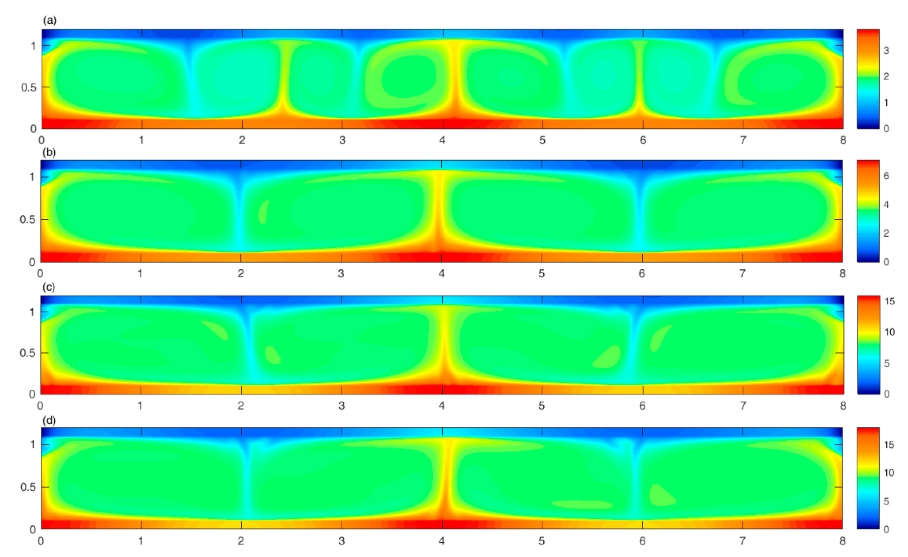
The fluid flow phenomena and occurrence of flow mode transition inside the annulus air gap of the solar collector are presented. All the simulations results are plotted after carrying grid independence tests with an optimum grid density of 240 × 12 nodes resolution. Transient iso-thermal contours on the computational domain of the numerical model are shown in Figure 7 for Ra = 105. Specifically in Figure 7d, the iso-thermal contours in the plate domain, fluid domain and glass domain are shown. In the following figures we have shown only the iso-thermal contours to clearly depict the occurrence of flow mode transition. As observed in this Figure, thermal plumes are formed where two stream function contours rotating in opposite directions intersect asymptotically. As well, the flow mode transition shown in Figure 8, where the mixing of 2 thermal plumes happens when the associated stream function contours coalesce into a single larger stream function contour. Similar fluid flow behaviour is also observed in the annulus gap of solar collectors in a previous CFD study [12]. The total transient behaviour of the convection fluid flow inside the annulus air gap can be classified into 3 stages.
- Flow development stage;
- Flow mode transition stage;
- Fully developed stage.
Typically for low Ra flows, where Ra less than critical Rayleigh number Racr, fluid is completely stable and flow does not occur, i.e., the heat transfer occurs completely due to conduction through air layers and the resultant Nu is zero. As Ra increases just greater than Racr, the gravitational forces become more dominant, instability sets in and Rayleigh-Benard convection cells appear. This phenomenon is called Rayleigh-Benard instability. This is when convection heat flow starts and the temperature starts rising from the absorber plate towards the glass cover, as shown in Figure 7a. The flow developmental stage is the stage starting from the occurrance of Raylieigh-Benard instability to the occurance of 1st flow mode transition. Flow mode transition stage is defined as the time period during which flow mode transitions occur and finally the steady state heat transfer is reached. As observed in the isothermal contours for low Ra at Ra = 105, the flow development stage has an approximate time period of 1.2 ND time units, as seen from the Nu diagram when the first flow mode transition occurs, followed by the flow mode transition stage where multiple Rayleigh Benard convection cells coalesce into single cells. The time period for the flow mode transition stage is approximately from 1.24 ND time units to 2.35 ND time units. As seen in Figure 8, 2 flow mode transitions occur at 1.24 s and 2.35 s respectively. As seen in Figure 9 left, the flow mode transition is also characterised by a decrease in Nu from 6.1 to 5.8 for the 1st flow mode transition and further decreases from 5.8 to 5.2 in the 2nd flow mode transition. The 3rd stage of transient flow is the fully developed stage where heat is transferred from the absorber plate to the glass cover via fluid flow configuration after the completion of all flow mode transitions, as shown in Figure 8d, for the case of Ra = 105. It is in the fully developed stage when the bulk of the heat transfer takes place from the absorber plate to the glass cover.
For the case of Ra = 106, the flow development stage and flow mode transition stages are instantaneous, as can be verified from isothermal contours in Figure 10. The flow mode transition occurs below 1 s and the bulk of the heat transfer occurs through fluid flow configurations, shown after 1 s. In addition, as seen in Figure 8b–d, the thermal plumes continuously oscillate after the developmental stage, resulting in the oscillating nature of the Nu value seen in Figure 9 right. This behaviour is also confirmed for higher Ra flows for triangular enclosures [31]. As Ra increases, the flow mode transitions happen instantly and the flow oscillates with a periodic behaviour, indicating a turbulent flow phenomenon at a higher absorber plate temperature with reference to the ambient or glass cover temperature.
Another important feature of increasing Ra is the reduction in both velocity and thermal boundary layer thickness of fluid flow contours. As observed in Figure 7 and Figure 10, as Ra increases, the boundary layer thickness near the solid surfaces and also the thickness of the thermal plumes significantly decrease. This is also associated with a corresponding increase in the size and strength of the stream function contours and also steep temperature gradients are formed in the boundary layers. In all the cases studied here, with an increase in Ra, the boundary layer thickness decreases and the Nu increases.
4. Conclusions
A fourth order accurate numerical method in both space and time is developed to evaluate the turbulent and transient behaviour of natural convection flow inside the air gap of a FPSC. The developed method could accurately model the steady state response of the solar collector with an error limit of 5% when compared with Mullick & Samdarshi [29]. It was observed that the transient state of fluid flow behaviour inside the air gap exists in three stages i.e., flow development stage, flow mode transition stage and fully developed stage. It was observed that flow mode transitions are associated with a reduction of Nusselt numbers and the associated convection heat transfer. Also flow mode transitions are preferable for reducing the convection heat transfer and subsequently the convection heat loss and thus improving the efficiency of the FPSC. Overall, the developed method could accurately predict the transient behaviour of fluid flow inside the air gap of the FPSC and offer new mechanisms to optimise and reduce the convection heat transfer loss in the solar collectors, and thus improving the overall conversion efficiency of the solar collectors.
Author Contributions
Conceptualization, N.B.B., T.A. and A.G.; methodology, N.B.B., T.A. and A.G; validation, N.B.B. and T.A.; writing—original draft preparation, N.B.B., T.A. and P.B.; writing—review and editing, N.B.B., T.A. and P.B.; All authors have read and agreed to the published version of the manuscript.
Funding
This research received no external funding.
Institutional Review Board Statement
Not applicable.
Informed Consent Statement
Not applicable.
Conflicts of Interest
The authors declare no conflict of interest.
Nomenclature
| Ar | Aspect Ratio (L/H) | X,Y | Non dimensional coordinates |
| Bi | Biot number | α | Thermal diffusivity, m2/s |
| Cp | Specific heat capacity, J/kg·K | β | Thermal expansion coefficient, 1/K |
| g | Gravitational force, m/s2 | γ | Angle of inclination of enclosure, °deg |
| Gr | Grashof number | ε | Numerical tolerance limit |
| h | Convective heat transfer coef., W/(m2·K) | θ | Non dimensional temperature |
| H | Height of respective domain | ν | Kinematic viscosity, m2/s |
| L | Length of enclosure | ρ | Density, kg/m3 |
| K | Thermal conductivity, W/(m·K) | τ | Non dimensional time |
| KΦ | Diffusion coefficient | ψ | Stream function |
| n | Time step | Ψ | Non dimensional streamfunction |
| N | Number of tubes | ω | vorticity |
| Nu | Nusselt number | Ω | Non dimensional vorticity |
| p | Pressure, N/m2 | Φ | General conservation variable |
| Pr | Prandtl number | ∇2 | Laplacian operator |
| q” | Heat flux, W/m2 | Order of discretisation | |
| Q | Non dimensional Heat flux | Subscripts/Superscripts | |
| R | Residual | o | Reference condition |
| Ra | Rayleigh number | amb | Ambient |
| SΦ | Transport eqn. source term | f | fluid |
| t | Time, sec | fp | fluid to plate |
| T | Temperature, K | fg | fluid to glass |
| Velocity vector, m/s | g | glass | |
| u,v | Velocity components, m/s | p | plate |
| Non dimensional velocity, m/s | S | Solar | |
| U,V | Non dimensional v components, m/s | t | tube |
| x,y | coordinates | w | water |
References
- Duffie, J.A.; Beckman, W.A. Solar Engineering of Thermal Processes; John Wiley & Sons: Hoboken, NJ, USA, 2013. [Google Scholar]
- Smith, J.G. Comparison of Transient Models for Flat-Plates and Trough Concentrators. J. Sol. Energy Eng. 1986, 108, 341–344. [Google Scholar] [CrossRef]
- Tagliafico, L.A.; Scarpa, F.; De Rosa, M. Dynamic thermal models and CFD analysis for flat-plate thermal solar collectors—A review. Renew. Sustain. Energy Rev. 2014, 30, 526–537. [Google Scholar] [CrossRef]
- Close, D. A design approach for solar processes. Sol. Energy 1967, 11, 112–122. [Google Scholar] [CrossRef]
- Klein, S. Calculation of flat-plate collector loss coefficients. Sol. Energy 1975, 17, 79–80. [Google Scholar] [CrossRef]
- Morrison, G.; Ranatunga, D. Transient response of thermosyphon solar collectors. Sol. Energy 1980, 24, 55–61. [Google Scholar] [CrossRef]
- Oliva, A.; Costa, M.; Segarra, C. Numerical simulation of solar collectors: The effect of nonuniform and nonsteady state of the boundary conditions. Sol. Energy 1991, 47, 359–373. [Google Scholar] [CrossRef]
- Ouzzane, M.; Galanis, N. Numerical Analysis Of Mixed Convection In Inclined Tubes With External Longitudinal Fins. Sol. Energy 2001, 71, 199–211. [Google Scholar] [CrossRef]
- Ramírez-Minguela, J.; Alfaro-Ayala, J.; Rangel-Hernandez, V.H.; Uribe-Ramírez, A.; Mendoza-Miranda, J.; Pérez-García, V.; Belman, J. Comparison of the thermo-hydraulic performance and the entropy generation rate for two types of low temperature solar collectors using CFD. Sol. Energy 2018, 166, 123–137. [Google Scholar] [CrossRef]
- Allan, J.; Dehouche, Z.; Stankovice, S.; Harries, A. Computational Fluid Dynamics Simulation and Experimental Study of Key Design Parameters of Solar Thermal Collectors. J. Sol. Energy Eng. 2017, 139, 051001. [Google Scholar] [CrossRef]
- Cerón, J.; Pérez-García, J.; Solano, J.; García, A.; Herrero-Martín, R. A coupled numerical model for tube-on-sheet flat-plate solar liquid collectors. Analysis and validation of the heat transfer mechanisms. Appl. Energy 2015, 140, 275–287. [Google Scholar] [CrossRef]
- Jiandong, Z.; Hanzhong, T.; Susu, C. Numerical simulation for structural parameters of flat-plate solar collector. Sol. Energy 2015, 117, 192–202. [Google Scholar] [CrossRef]
- Dović, D.; Andrassy, M. Numerically assisted analysis of flat and corrugated plate solar collectors thermal performances. Sol. Energy 2012, 86, 2416–2431. [Google Scholar] [CrossRef]
- Fan, J.; Shah, L.J.; Furbo, S. Flow distribution in a solar collector panel with horizontally inclined absorber strips. Sol. Energy 2007, 81, 1501–1511. [Google Scholar] [CrossRef]
- Martinopoulos, G.; Missirlis, D.; Tsilingiridis, G.; Yakinthos, K.; Kyriakis, N. CFD modeling of a polymer solar collector. Renew. Energy 2010, 35, 1499–1508. [Google Scholar] [CrossRef]
- Selmi, M.; Al-Khawaja, M.J.; Marafia, A. Validation of CFD simulation for flat plate solar energy collector. Renew. Energy 2008, 33, 383–387. [Google Scholar] [CrossRef]
- Sahin, M.; Owens, R.G. A novel fully implicit finite volume method applied to the lid-driven cavity problem? Part I: High Reynolds number flow calculations. Int. J. Numer. Methods Fluids 2003, 42, 57–77. [Google Scholar] [CrossRef]
- Balam, N.B.; Gupta, A. A fourth-order accurate finite difference method to evaluate the true tran-sient behaviour of natural convection flow in enclosures. Int. J. Numer. Methods Heat Fluid Flow 2020, 33, 1233–1290. [Google Scholar]
- Davis, G.D.V. Natural convection of air in a square cavity: A bench mark numerical solution. Int. J. Numer. Methods Fluids 1983, 3, 249–264. [Google Scholar] [CrossRef]
- Le Quéré, P. Accurate solutions to the square thermally driven cavity at high Rayleigh number. Comput. Fluids 1991, 20, 29–41. [Google Scholar] [CrossRef]
- Syrjälä, S. Higher order penalty-galerkin finite element approach to laminar natural convection in a square cavity. Numer. Heat Transf. Part A Appl. 1996, 29, 197–210. [Google Scholar] [CrossRef]
- Tian, Z.; Ge, Y. A fourth-order compact finite difference scheme for the steady stream function-vorticity formulation of the Navier-Stokes/Boussinesq equations. Int. J. Numer. Methods Fluids 2003, 41, 495–518. [Google Scholar] [CrossRef]
- Kalita, J.C.; Dalal, D.C.; Dass, A.K. Fully compact higher-order computation of steady-state natural convection in a square cavity. Phys. Rev. E 2001, 64, 066703. [Google Scholar] [CrossRef]
- Kondo, N. Numerical simulation of unsteady natural convection in a square cavity by the third-order upwind finite element method. Int. J. Comput. Fluid Dyn. 1994, 3, 281–302. [Google Scholar] [CrossRef]
- Mayne, D.A.; Usmani, A.; Crapper, M. h-adaptive finite element solution of high Rayleigh number thermally driven cavity problem. Int. J. Numer. Methods Heat Fluid Flow 2000, 10, 598–615. [Google Scholar] [CrossRef] [Green Version]
- Yapici, K.; Obut, S. Benchmark results for natural and mixed convection heat transfer in a cavity. Int. J. Numer. Methods Heat Fluid Flow 2015, 25, 998–1029. [Google Scholar] [CrossRef]
- Wan, D.C.; Patnaik, B.S.V.; Wei, G.W. A new benchmark quality solution for the buoyancy-driven cavity by discrete singular convolution. Numer. Heat Transf. Part B Fundam. 2001, 40, 199–228. [Google Scholar] [CrossRef]
- Christon, M.A.; Gresho, P.M.; Sutton, S.B. Computational predictability of time-dependent natural convection flows in enclosures (including a benchmark solution). Int. J. Numer. Methods Fluids 2002, 40, 953–980. [Google Scholar] [CrossRef]
- Mullick, S.C.; Samdarshi, S.K. An Improved Technique for Computing the Top Heat Loss Factor of a Flat-Plate Collector With a Single Glazing. J. Sol. Energy Eng. 1988, 110, 262–267. [Google Scholar] [CrossRef]
- Subiantoro, A.; Ooi, K.T. Analytical models for the computation and optimization of single and double glazing flat plate solar collectors with normal and small air gap spacing. Appl. Energy 2013, 104, 392–399. [Google Scholar] [CrossRef]
- Holtzman, G.A.; Hill, R.W.; Ball, K.S. Laminar Natural Convection in Isosceles Triangular Enclosures Heated From Below and Symmetrically Cooled From Above. J. Heat Transf. 2000, 122, 485–491. [Google Scholar] [CrossRef]
Figure 1.
Geometry and Coordinate system for square domain.
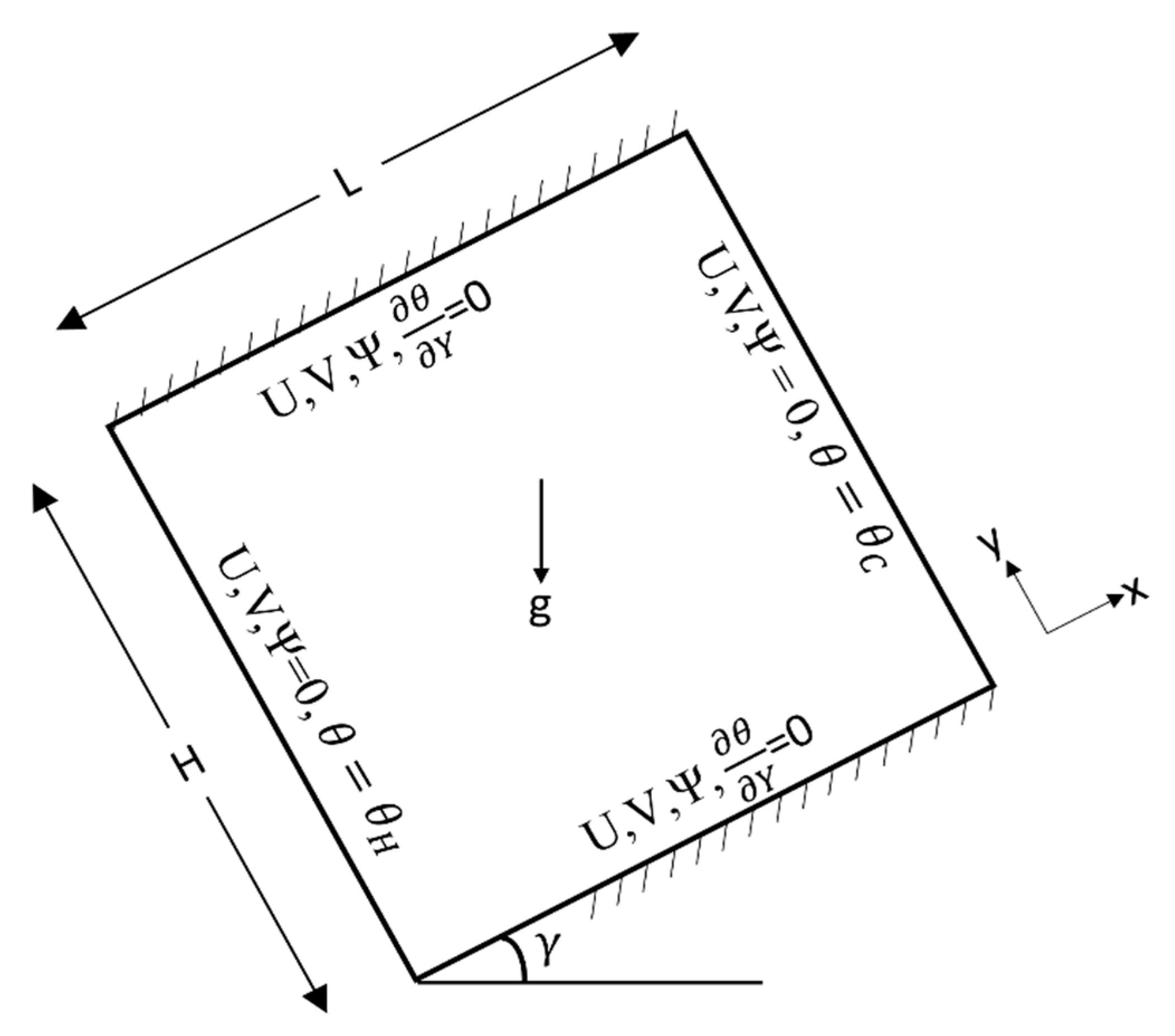
Figure 2.
Streamlines (left), Temperature contours (middle), Vorticity contours (right) for (a) Ra = 107 and (b) Ra = 108.
Figure 2.
Streamlines (left), Temperature contours (middle), Vorticity contours (right) for (a) Ra = 107 and (b) Ra = 108.
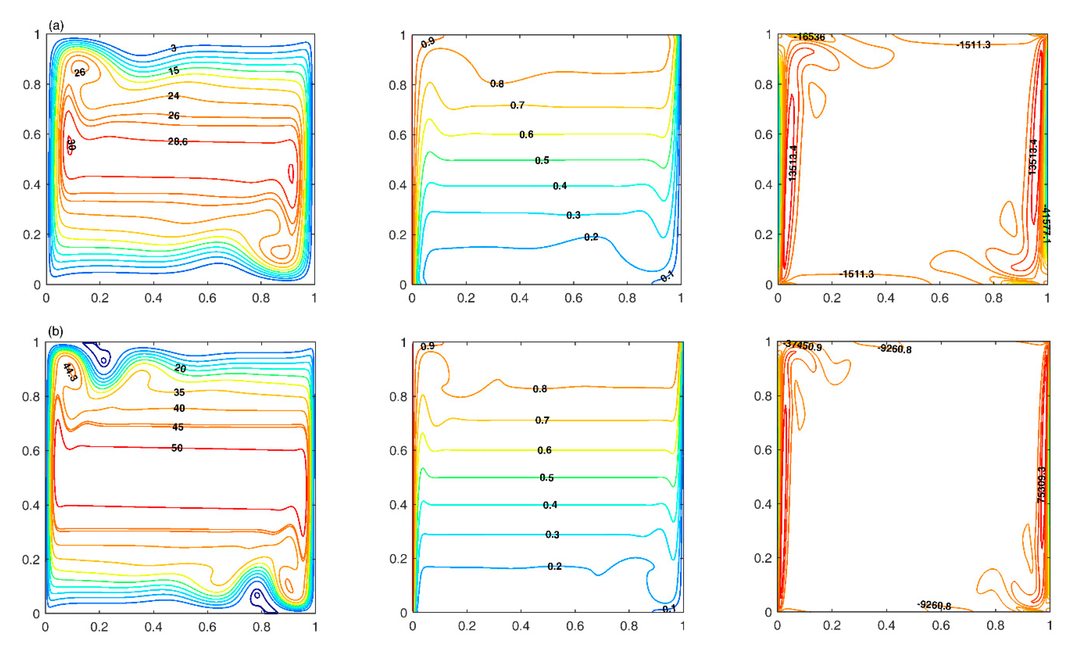
Figure 3.
Differentially heated enclosure with 8:1 aspect ratio (not to scale), with insulated horizontal walls and isothermal vertical walls.
Figure 3.
Differentially heated enclosure with 8:1 aspect ratio (not to scale), with insulated horizontal walls and isothermal vertical walls.

Figure 4.
Variation of Streamlines (a–d) and Temperature contours (e–h) during a time period at time instants 3486.7, 3487.9, 3489.1, 3490.2 ND time units respectively of a total time period of 3.412 ND time units.
Figure 4.
Variation of Streamlines (a–d) and Temperature contours (e–h) during a time period at time instants 3486.7, 3487.9, 3489.1, 3490.2 ND time units respectively of a total time period of 3.412 ND time units.
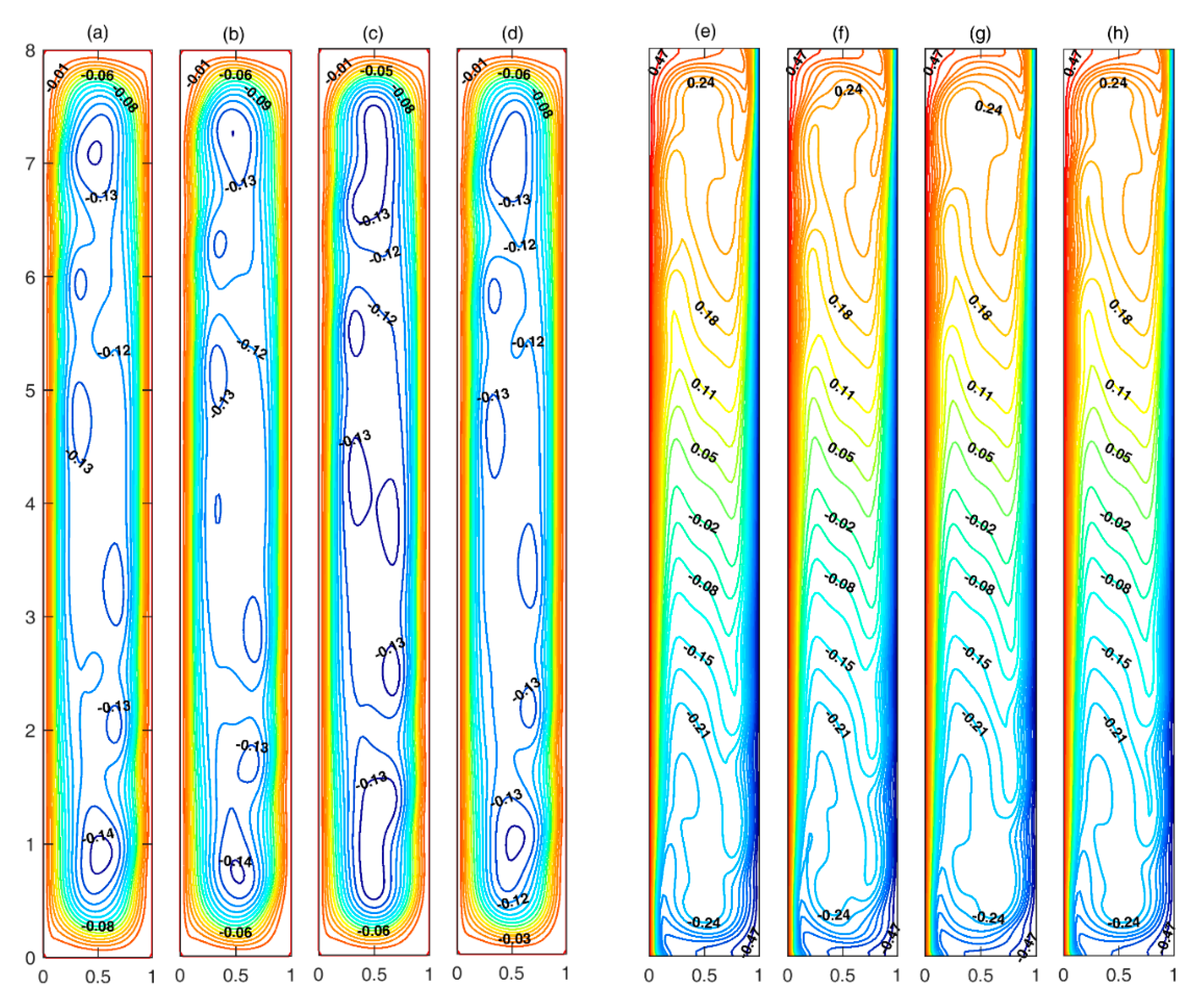
Figure 5.
(left) Oscillation of ND Temperature values and (right) Oscillation of ND U values at designated points 1–5 with reference to the ND Time indicating the oscillatory behaviour of the solution and the occurrence of convergence.
Figure 5.
(left) Oscillation of ND Temperature values and (right) Oscillation of ND U values at designated points 1–5 with reference to the ND Time indicating the oscillatory behaviour of the solution and the occurrence of convergence.
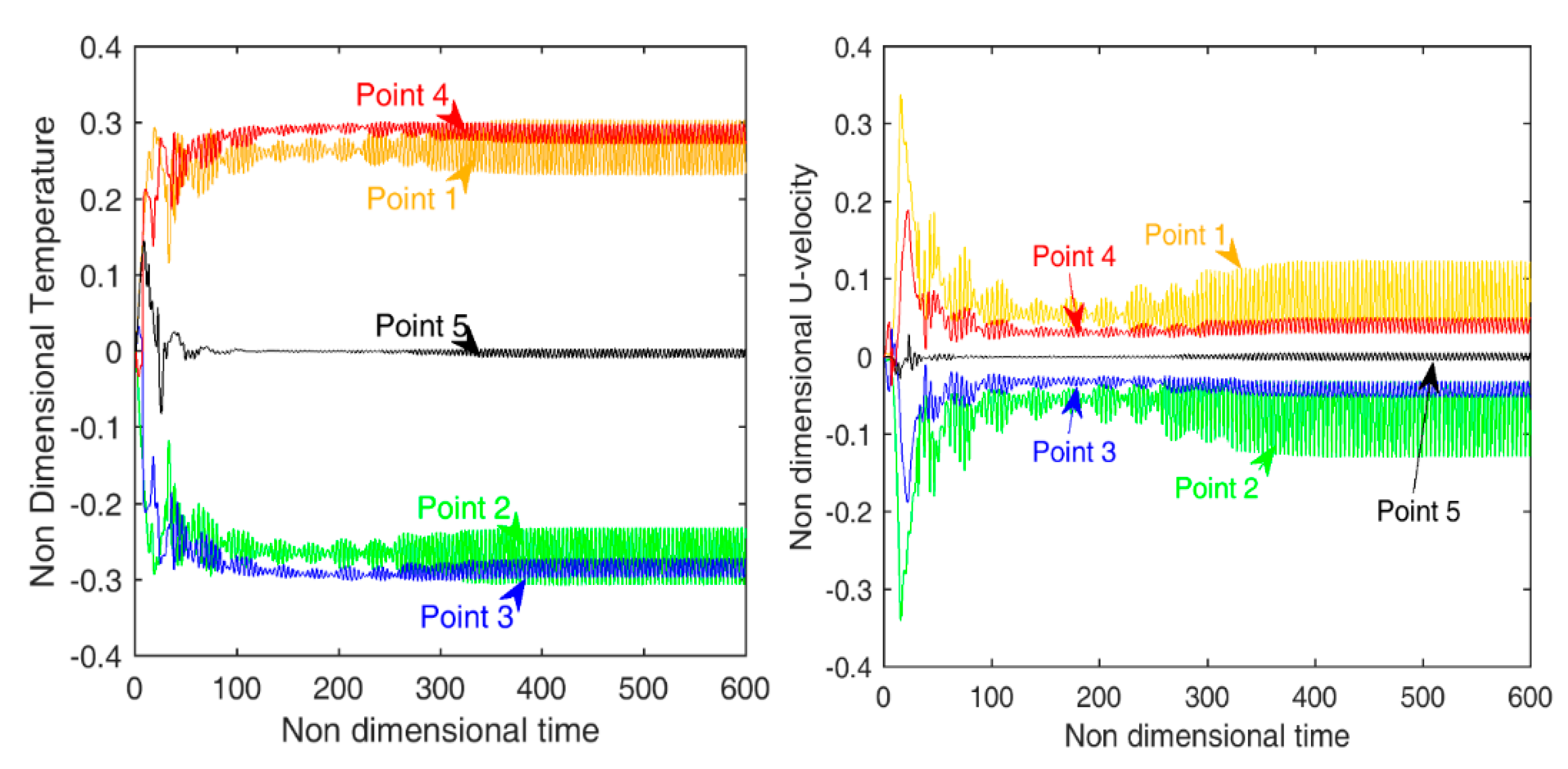
Figure 6.
Schematic diagram of FPSC with boundary conditions.
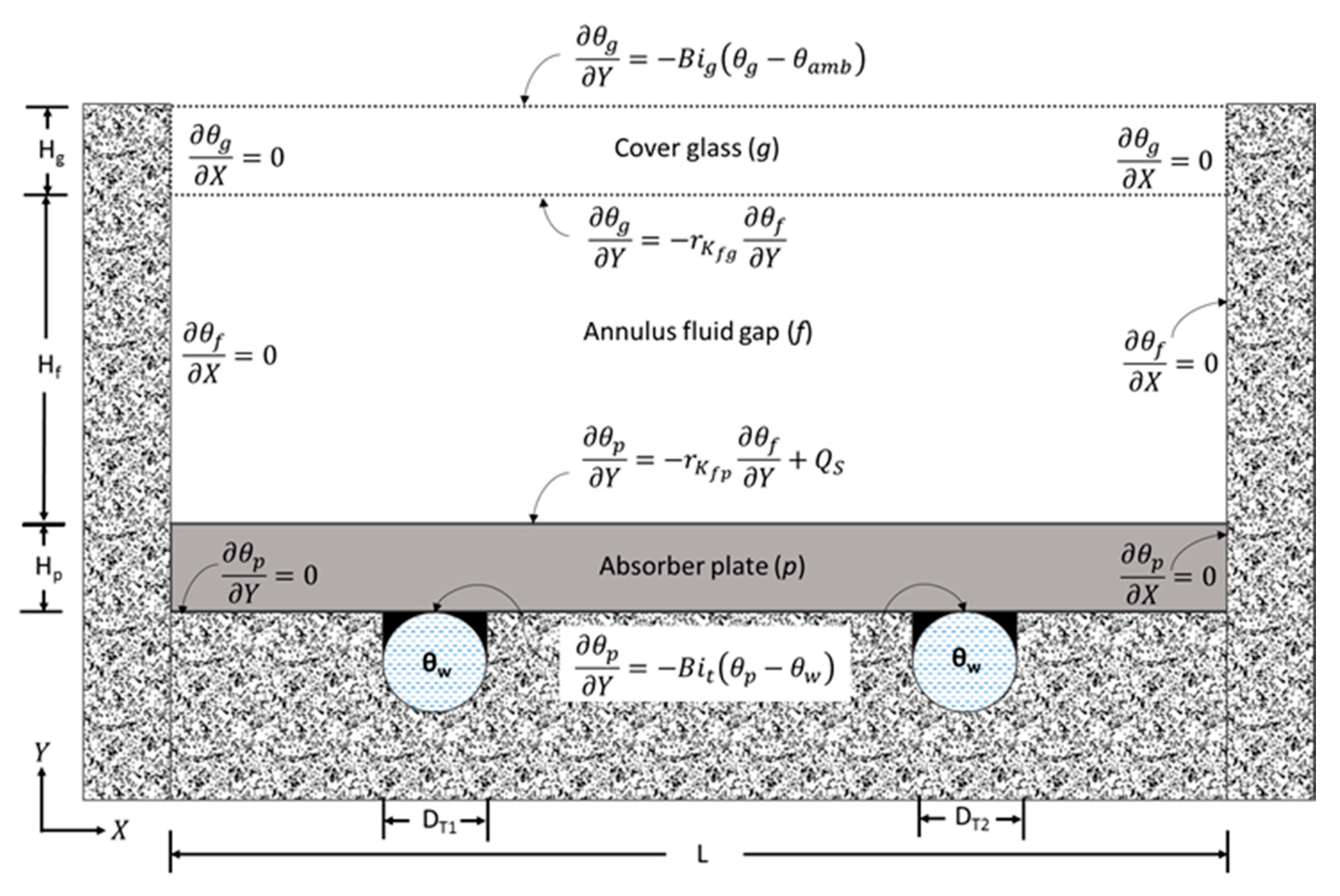
Figure 7.
Isothermal contours for Ra = 105, at time period of (a) 0.5 s, (b) 1 s, (c) 2 s, (d) 3 s, showing the plate domain, annulus air gap i.e., fluid domain and glass domain.
Figure 7.
Isothermal contours for Ra = 105, at time period of (a) 0.5 s, (b) 1 s, (c) 2 s, (d) 3 s, showing the plate domain, annulus air gap i.e., fluid domain and glass domain.

Figure 8.
Occurrence of flow mode transition at time period (a) 1.24 s and (b) 1.25 s, and at time period (c) 2.35 s and (d) 2.36 s.
Figure 8.
Occurrence of flow mode transition at time period (a) 1.24 s and (b) 1.25 s, and at time period (c) 2.35 s and (d) 2.36 s.

Figure 9.
Nu variation with non-dimensional time for Ra = 105 (left) and Ra = 106 (right).

Figure 10.
Iso-thermal contours for Ra = 106, at time period of (a) 0.5 s, (b) 1 s, (c) 4 s, (d) 9 s.
Figure 10.
Iso-thermal contours for Ra = 106, at time period of (a) 0.5 s, (b) 1 s, (c) 4 s, (d) 9 s.

Table 1.
Ra = 107.
| Reference | |||||||
|---|---|---|---|---|---|---|---|
| Present Study | 29.3558 | 29.945 | 144.3603 (0.8875) | 691.8772 (0.0188) | 16.6505 | 39.5199 (0.0179) | 1.3374 (1.000) |
| Le Quéré [20] | 29.361 | 30.165 | 148.59 (0.879) | 699.17 (0.021) | 16.523 | 39.39 (0.018) | 1.366 (1) |
| Syrjälä [21] | 29.3616 | ---- | 148.593 (0.8794) | 699.506 (0.0213) | 16.5299 | ---- | ---- |
| Tian and Ge [22] | 29.3562 | 30.155 | 148.5695 (0.8794) | 699.2991 (0.0213) | 16.5106 | 39.2540 (0.0179) | 1.3655 (1) |
| Kalita et al. [23] | 29.382 | ---- | 155.82 (0.863) | 696.238 (0.025) | 16.075 | 34.925 (0.025) | 1.509 (1) |
| Kondo [24] | ---- | ---- | 149.7153 (0.8763) | 702.6753 (0.0187) | 16.5123 | 38.8717 (0.0187) | 1.3767 (1) |
| Mayne et al. [25] | ---- | ---- | 145.2666 (0.8845) | 703.2526 (0.0215) | 16.3869 | 41.0247 (0.0390) | 1.3799 (1) |
| Yapici and Obut [26] | 29.3631 | 30.168 | 148.6179 (0.8801) | 699.4755 (0.0213) | 16.5479 | 39.4796 (0.0174) | 1.3661 (0.9995) |
Table 2.
Ra = 108.
| Reference | |||||||
|---|---|---|---|---|---|---|---|
| Present Study | 52.2217 | 53.718 | 316.3440 (0.9250) | 2218.115 (0.0125) | 30.1348 | 103.6505 (0.000) | 1.9072 (1.000) |
| Le Quéré [20] | 52.32 | 53.85 | 321.9 (0.928) | 2222 (0.012) | 30.225 | 87.24 (0.008) | 1.919 (1) |
| Kondo [24] | ---- | ---- | 315.2603 (0.9389) | 2241.1841 (0.0136) | 30.1901 | 84.3960 (0.0100) | 2.0798 (1) |
| Mayne et al. [25] | ---- | ---- | 283.0689 (0.9455) | 2223.4424 (0.0130) | 29.6526 | 91.2095 (0.0670) | 2.0440 (1) |
| Wan et al. [27] | ---- | ---- | 296.71 (0.93) | 2259.08 (0.012) | 31.486 | 91.16 (0.010) | 1.766 (1) |
| Yapici and Obut [26] | 52.3577 | 53.883 | 323.1085 (0.9279) | 2220.4766 (0.0125) | 30.3056 | 88.1516 (0.0079) | 1.9172 (0.9995) |
Table 3.
ND Coordinates for the time history points shown in Figure 3.
Table 3.
ND Coordinates for the time history points shown in Figure 3.
| Point | x-Coordinate | y-Coordinate |
|---|---|---|
| 1 | 0.1810 | 7.3700 |
| 2 | 0.8190 | 0.6300 |
| 3 | 0.1810 | 0.6300 |
| 4 | 0.8190 | 7.3700 |
| 5 | 0.1810 | 4.0000 |
Table 4.
Comparison of Point data at reference point 1 with standard results available from Christon et al. [28].
Table 4.
Comparison of Point data at reference point 1 with standard results available from Christon et al. [28].
| Contributor | ||||||||
|---|---|---|---|---|---|---|---|---|
| Present Study | 0.057013 | 0.056342 | 0.265781 | 0.043944 | −0.073503 | 0.007189 | −2.351614 | 1.108430 |
| Le Quere | 0.056356 | 0.054828 | 0.265480 | 0.042740 | ---- | ---- | ---- | ---- |
| Christon | 0.058670 | 0.055120 | 0.264140 | 0.042420 | −0.07394 | 0.007106 | −2.1213 | 0.9710 |
| Jhonston | 0.056160 | 0.054520 | 0.264700 | 0.042680 | −0.07348 | 0.006856 | −2.3620 | 0.9940 |
| Davis | 0.056300 | 0.054200 | 0.265500 | 0.042200 | ---- | ---- | ---- | ---- |
| Gresho | 0.056493 | 0.055414 | 0.265722 | 0.043144 | −0.07439 | 0.007100 | −2.4455 | 1.0810 |
Table 5.
Top heat loss coefficient comparison (Ut: W/m2/K).
| Rayleigh No. | 1 | 100 | 1000 | 2500 |
|---|---|---|---|---|
| Mullick & Samdarshi [29] | 13 | 6.5 | 5.5 | 5.4 |
| Present study | 11.5 | 6.0 | 5.3 | 5.2 |
| |%| Difference | 13 | 8.3 | 3.8 | 3.85 |
Publisher’s Note: MDPI stays neutral with regard to jurisdictional claims in published maps and institutional affiliations. |
© 2021 by the authors. Licensee MDPI, Basel, Switzerland. This article is an open access article distributed under the terms and conditions of the Creative Commons Attribution (CC BY) license (https://creativecommons.org/licenses/by/4.0/).
Share and Cite
MDPI and ACS Style
Balam, N.B.; Alam, T.; Gupta, A.; Blecich, P. Higher Order Accurate Transient Numerical Model to Evaluate the Natural Convection Heat Transfer in Flat Plate Solar Collector. Processes 2021, 9, 1508. https://doi.org/10.3390/pr9091508
AMA Style
Balam NB, Alam T, Gupta A, Blecich P. Higher Order Accurate Transient Numerical Model to Evaluate the Natural Convection Heat Transfer in Flat Plate Solar Collector. Processes. 2021; 9(9):1508. https://doi.org/10.3390/pr9091508
Chicago/Turabian StyleBalam, Nagesh Babu, Tabish Alam, Akhilesh Gupta, and Paolo Blecich. 2021. "Higher Order Accurate Transient Numerical Model to Evaluate the Natural Convection Heat Transfer in Flat Plate Solar Collector" Processes 9, no. 9: 1508. https://doi.org/10.3390/pr9091508
Note that from the first issue of 2016, this journal uses article numbers instead of page numbers. See further details here.