Article

Identifying the Early Post-Mortem VOC Profile from Cadavers in a Morgue Environment Using Comprehensive Two-Dimensional Gas Chromatography

1
Département de Chimie, Biochimie et Physique, Université du Québec à Trois-Rivières, 3351 Boul. des Forges, Trois-Rivières, QC G8Z 4M3, Canada
2
Department of Forensic Science, School of Science, G H Raisoni University, Amravati 444701, Maharashtra, India
3
Department of Mathematics, Trent University, 1600 West Bank Drive, Peterborough, ON K9L 0G2, Canada
4
Department of Chemistry and Biochemistry, University of Windsor, Faculty of Science, Sunset Avenue, Windsor, ON N9B 3P4, Canada
*
Author to whom correspondence should be addressed.
Separations 2023, 10(11), 566; https://doi.org/10.3390/separations10110566
Submission received: 27 September 2023 / Revised: 31 October 2023 / Accepted: 8 November 2023 / Published: 10 November 2023
(This article belongs to the Special Issue Chemical Separations in Criminalistics)

Abstract

:
Understanding the VOC profile released during the early post-mortem period is essential for applications in training human remains detection dogs and urban search and rescue operations (USAR) to rapidly locate living and deceased victims. Human cadavers were sampled at the UQTR morgue within a 0–72 h post-mortem interval. VOC samples were collected from the headspace above the cadavers, using Tenax TA/Carbograph 5TD dual sorbent tubes, and analyzed using GC×GC-TOFMS. Multiple data processing steps, including peak table alignment and filtering, were undertaken using LECO ChromaToF and custom scripts in R programming language. This study identified 104 prevalent VOCs, some of which are linked to human decomposition, while others are connected to the persistence of living scent. Principal Component Analysis (PCA) further highlighted that VOC profiles can change dynamically over time, even in a controlled setting. The findings underscore the complexity and variability in VOC profiles during the early post-mortem period. This variability is influenced by multiple factors including the individual’s biological and physiological conditions. Despite the challenges in characterizing these profiles, the identified VOCs could potentially serve as markers in forensic applications. The study also highlights the need for additional research to build a dataset of VOCs for more robust forensic applications.

1. Introduction

The human body undergoes the process of autolysis and putrefaction, predominantly in the absence of oxygen [1,2]. The simultaneous degradation of proteins, lipids, and carbohydrates in the absence of oxygen produces various volatile and semi-volatile organic compounds (VOCs and SVOCs) as well as inorganic compounds that comprise the characteristic odor of decomposition [3,4,5]. Studies conducted on decomposition odor have focused on the characterization of VOCs released during the entire process (fresh to skeletonization) [6,7,8,9]. The early post-mortem period encompasses the fresh stage of decomposition. Understanding the VOC profile released during the early post-mortem period is essential for applications in training human remains detection (HRD) dogs and urban search and rescue operations (USAR) to rapidly locate living and deceased victims [10]. In the context of urban search and rescue operations (USAR), the initial hours following a mass disaster are crucial, as the chances of survival for victims decrease significantly after the first 48 h. The chances of survival for a human can vary and depend upon the availability of food, water, and oxygen [10,11]. Therefore, there is a need for improved methods that can be applied during the first 72 h to rapidly locate live victims and human remains in a mass disaster scenario.
Characterizing the VOC profile released during the early post-mortem period is challenging as these processes are in the beginning stages, resulting in a lower abundance of VOCs in the profile, thereby adding to the analytical challenge. Due to ethical challenges related to the use of human remains, the use of cadavers to profile the odor released during the early post-mortem has been limited [8,12]. Statheropoulos et al. [13] and DeGreeff et al. [14] individually conducted research in a morgue to examine the VOC profile of cadavers during the early post-mortem period. Despite the low concentrations of VOCs, their experimental approach allowed for the collection and identification of VOCs associated with decomposition odor during the early post-mortem stage. However, the studies produced non-comparable results, which can be attributed to the use of different sample collection techniques (sorbent tubes vs. gauze pieces). The authors employed gas chromatography mass spectrometry (GC-MS) for sample analysis, but this analytical technique has limitations such as the potential for co-elution in complex mixtures, difficulty in managing the dynamic range of VOCs, complexities in background samples, and reduced sensitivity. These factors make it less than ideal for analyzing VOC samples collected during the early post-mortem period.
In the last decade, comprehensive two-dimensional gas chromatography-time-of-flight mass spectrometry (GC×GC-TOFMS) has become the preferred technique to study the decomposition VOC profile [7,8,9,12,15,16,17,18,19]. This analytical technique relies on two different columns with two different stationary phases serially connected via a modulator. The modulator traps the analytes as they elute from the first-dimension column (1D) and periodically injects the analytes onto the second-dimension column (2D) in a series of short pulses [19,20]. TOFMS is typically employed as the detection system for studies on decomposition odor as it offers fast acquisition rates required to characterize the very narrow 2D peaks. Moreover, TOFMS is a non-scanning MS that can acquire full mass spectrum because the entire mass range is sampled from the ion source at the same instant in time [19]. The analytical setup of this technique provides a better separation of analytes by enhancing selectivity, sensitivity, and peak capacity [21]. Thus, its application to the early post-mortem VOC profile of cadavers released in a controlled indoor environment (e.g., morgue) can assist in identifying the less abundant VOCs released in low concentrations during this period.
Natural (freezing) and chemical (embalming) techniques are used in a morgue to protect donated bodies from decomposition. Profiling VOCs from the cadavers during the early post-mortem period upon their arrival in the morgue (6–72 h) can provide a baseline VOC profile of a person soon after death and prior to these techniques being applied. This baseline VOC profile can be used to understand the transition of odor from the peri-mortem period to the post-mortem odor. This study aims to determine the VOCs released from human remains in a controlled environment in the absence of external factors that contribute to the decomposition process.

2. Materials and Methods

2.1. Experimental Design

The sample collection was conducted using donated human cadavers (henceforth referred to as donors) in the UQTR (Université du Québec a Trois-Rivières) morgue (UQTR Department of Anatomy). During this study, eight donors were sampled, of which four were females and four were males. Notably, the demographics of the donor population are narrow, primarily comprising elderly individuals who died of natural causes. The history of preserving these donors prior to their arrival at the morgue is unknown, but at most involves refrigeration only (not freezing or embalming). Regardless, they were all in the fresh stage of decomposition. The donors were sampled in a clean sterile indoor morgue environment, accessed by authorized personnel only. The donors arrived in a shroud material and their arrival was infrequent and occurred at varying post-mortem periods ranging from 12 to 72 h. The duration of their storage in the shroud prior to their arrival at the morgue varied. Thus, to address this variability, the shroud was opened for 5 min to minimize the influence of the shroud on VOC accumulation before collection at the UQTR morgue after the arrival of the donors.

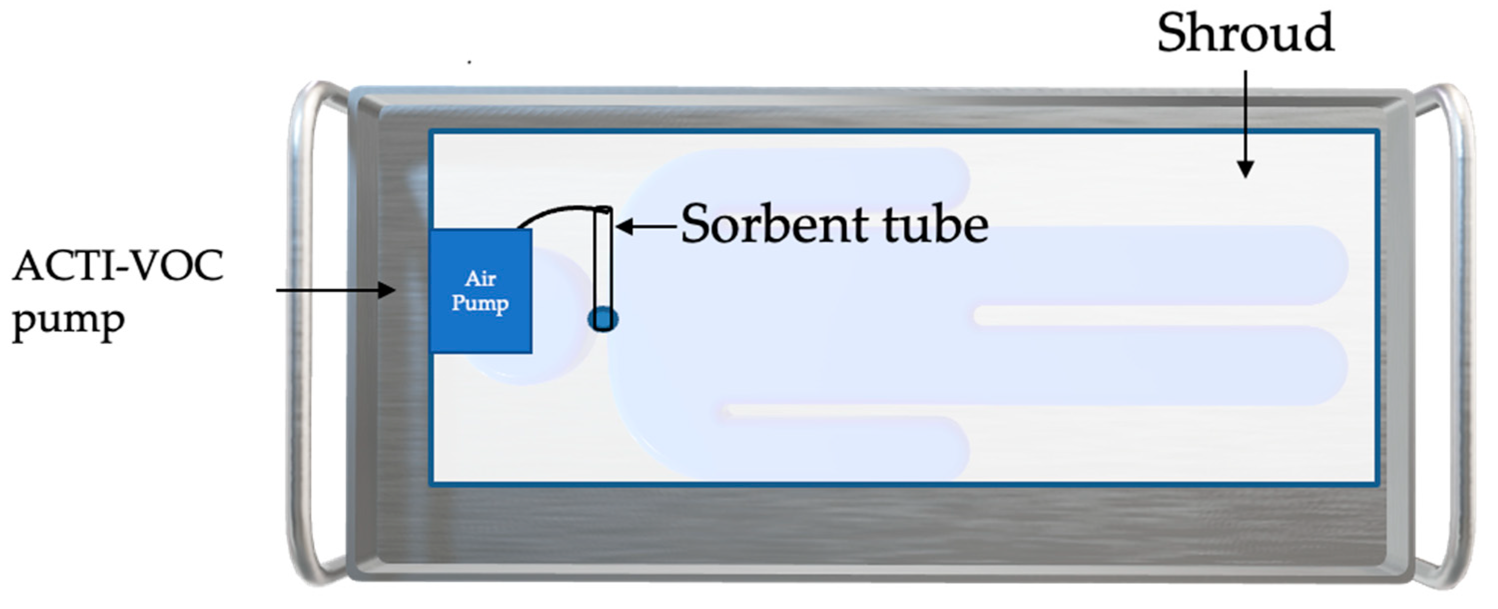
2.2. VOC Sample Collection

The headspace samples were dynamically collected onto the stainless-steel sorbent tube using an ACTI-VOC low flow pump (Markes International Ltd., Llantrisant, UK) to sample VOCs at a constant flow [7,9,12,16,17]. The shroud was resealed to create a headspace and the VOCs were accumulated for 20 min. A small opening was created over the upper chest region in the shroud, and one end of the Tenax TA/Carbograph 5TD dual sorbent tubes (Markes International Llantrisant, UK) was inserted in the headspace of the shroud. The other end was attached to an ACTI-VOC low flow pump (Markes International Ltd., Llantrisant, UK) (Figure 1) such that the sampling arrow was pointing towards the pump (Figure 1). The VOCs were collected at a constant flow rate of 100 mL/min and the sample volume collected was 1 L. The tubes were capped with brass storage caps, wrapped in aluminum foil, and stored in a glass jar for transportation to the laboratory (US EPA method TO-107) [22]. These sorbent tubes were stored in an airtight glass jar at 4 °C until analysis. Control samples comprised background VOC samples.

2.3. Standards

An internal standard consisting of 0.2 μL of 50 ppm bromobenzene (HPLC grade, Sigma-Aldrich, Oakville, ON, Canada) was prepared in methanol (HPLC Grade, Sigma-Aldrich, Oakville, ON, Canada) and injected onto each sorbent tube using an eVol® XR handheld automated analytical syringe (SGE Analytical Science, Wetherill Park, NSW, Australia) for the purpose of internal standard normalization of analytes prior to analysis. Further, three custom-made decomposition standard mixes containing 25 compounds belonging to different compound classes (e.g., alcohols, esters, aldehydes, etc.) were purchased through Restek (Table S1). These compounds were previously identified through cadaveric studies [9,23].

2.4. VOC Analysis

The analytes collected on the sorbent tubes were thermally desorbed using a TD100-xr autosampler thermal desorption unit (Markes International, Llantrisant, UK) and analyzed using the Pegasus® BT 4D GC×GC-TOFMS (Leco Instruments, St. Joseph, MI, USA). A 1.2 m uncoated silica-fused transfer line connected the TD100-xr to the Pegasus® BT 4D GC×GC-TOFMS system. This transfer line was maintained at 150 °C and the TD100-xr was controlled by the Markes Instrument Control (MIC) (version 2.0). ChromaTOF® (version 5.51.6.0; LECO Instruments, St. Joseph, MI, USA) was used to control the Pegasus® BT 4D GC×GC-TOFMS. The sorbent tubes were thermally desorbed at 300 °C for 4 min onto the general-purpose cold trap held at −10 °C followed by trap desorption at 280 °C for 3 min. A mid-polar 30 m × 0.250 mm (ID), 1.40 μm film thickness Rxi®-624Sil MS column (Restek Corporation, Bellefonte, PA, USA) was used in the first dimension (1D). A polar 2 m × 0.250 mm ID, 0.25 μm film thickness Stabilwax® column (Restek Corporation, Bellefonte, PA, USA) was used in the second dimension (2D). A SilTite μ-Union (Restek Corporation, Bellefonte, PA, USA) was used to connect the 1D and 2D columns. High-purity helium (Linde Inc, Trois-Rivières, QC, Canada) was used as the carrier gas at a constant pressure of 17.8 psi. The 2D oven temperature offset was +10 °C relative to the GC oven. The modulator temperature offset was +15 °C relative to the secondary oven and modulation period (PM) was 5 s with a 1.25 s hot and cold pulse time. The temperature of the MS transfer line and ion source was maintained at 250 °C, the electron ionization energy was 70 eV with an acquisition range of 29–300 amu and an acquisition rate of 250 spectra/s.

2.5. Data Processing

2.5.1. Data Processing in ChromaTOF (v.5.51; LECO)

Pegasus® BT GC×GC-TOFMS data were acquired and processed with ChromaTOF® (v.5.51; LECO). The data processing steps included non-targeted deconvolution (NTD®) peak finding with integration baseline; GC×GC subpeak combining; and library searching. During the NTD peak finding, the minimum S/N ratio of 1 was used for peak finding while for the integration baseline, the default option of ‘auto-calculated’ was selected. The minimum spectral match required to combine GC×GC sub-peaks was set at 650. Tentative identifications of peaks were made by matching them with 2017 NIST spectral libraries. The minimum similarity thresholds for spectral matches and peak assignments were set at 600 and 800, respectively. Lower primary match selection criteria for the S/N ratio were used during the data processing step to increase the library search results. Further alignment and data filtering steps at the peak table level were performed in RStudio Workbench (2022.02.2, build 485.pro2), as described below.

2.5.2. Data Processing in R

The current ChromaTOF software package (v.5.51) did not include LECO’s Statistical Compare package, an integrated software solution used for peak table alignment in various decomposition studies [8,9,12,16,17]. The absence of an integrated software solution led to the development of a series of peak table alignment scripts in the R programming language which would allow the alignment of peak tables across the samples using the peak table output. The peak tables of each sample with their respective replicates and controls were exported as xlsx files. The exported peak tables contained information including peak number; name; formula; retention times (RTs); 1st dimension retention times (RT1); 2nd dimension retention time (RT2); similarity; area; height; quant mass; base mass; quant S/N; and peak S/N.

Peak Table Alignment

The peak table alignment was based on retention times matching criteria and mass values (base mass and quant mass), following a spectral match performed with the NIST library. All the peaks within the peak table had a similarity and reverse spectral match factor >800 with the 2017 NIST spectral libraries. The retention time match criteria were set to 10 s in 1D and 0.06s in 2D. The values of retention time match criteria for 1D and 2D were derived from the retention time values of the internal standard and decomposition standard mix. A chromatographic region after 2500 s in the 1D was excluded from the alignment process, as the majority of the peaks identified after this period were not compounds of interest (e.g., siloxanes and non-detects).
Before peak alignment, the dataset was classified into controls and experimental classes. The control class comprised samples collected as background samples in the morgue. The experimental class consisted of donor samples collected in the morgue with their respective replicates. In the peak table alignment process, each peak was treated as unique and subjected to consistent pairwise comparisons across all samples in the class. Criteria such as name, minimum S/N of 100, retention time matching (10 s and 0.06 s), and mass values were employed for the consistent matching of integrated peaks within the sample and across all samples in the class. Once this was complete, and all identified peaks were isolated by sample, we proceeded to the second stage of the analysis, starting with a sliding window identification of commonality by compound. A sliding window function was used to verify the alignment of peaks within peak tables, as the alignment procedure resulted in multiple RTs and masses per NIST-detected compound. This function consisted of a rectangular window made up of the first and second retention time windows, as used in the retention time match criteria. For a given compound, the sliding window function found the highest number of incidences of any common mass within the rectangular window. The identified maximum window region was then analyzed to determine the centroid retention times, and the common mass of a given identified compound. All other “detections” were then removed from the dataset. This ensured that every single compound considered in the following stages had common detection identification, common mass, and retention times within the precision of the variation of the internal standard and decomposition standard mix. This should ensure, as much as is possible, that any compound detections in the following are truly considering the same compound, across both samples and controls. The samples were normalized to the peak areas of the internal standard following the peak table alignment.

Data Filtering and Sample/Control Couple Comparison

Control samples were compared to triplicate experimental samples to remove background peaks and retain relevant peaks. Criteria such as mass values, peak area, and S/N ratio were used for the comparison and calculation of peak abundance. Peaks uniquely identified in control samples were filtered out. Peaks present in both control and experimental samples were retained in the experimental sample only if their abundance was at least twofold higher than the control sample. After filtering based on the control, the triplicate samples were combined, and only peaks present in all three triplicate samples were retained. Average peak area was calculated for each compound and triplicate to facilitate subsequent analysis. After applying the cleaning procedure, the relevant outputs for each donor were merged based on their presence in the respective replicate samples. Compounds such as siloxanes, oxygen peaks, acetone, etc., were excluded. Subsequently, individual donor data frames were merged into a single file containing a consolidated list of identified compounds across all donors. Detailed scripts can be found on GitHub [https://github.com/wesleyburr/GCxGC_Morgue_RESTES] (accessed on 30 October 2023).
Principal Component Analysis (PCA) was performed using the Unscrambler X (version 10.5; CAMO Software, Oslo, Norway). Mean centering, standard deviation scaling, and unit vector normalization were all applied to the datasets prior to PCA. The data contained no outliers by way of Hotelling’s T2 95% confidence limit.

3. Results

The VOC profiles were collected from donors in the fresh stage of decomposition, excluding donor H1. Donor H1 was not discovered for approximately 24 h and showed initial signs of autolysis and putrefaction at the time of sample collection. In contrast, all other donors exhibited only the triad changes such as livor mortis, algor mortis, and rigor mortis. After data-filtering and sample-control comparative analysis, a compound list was generated. To minimize the impact of background VOCs related to the shroud material, a manual review was conducted on the compounds that were exclusively identified in the experimental samples. Subsequently, VOCs associated with the background were systematically excluded from the final list. In this study, the number of VOCs present in the sample represented the VOC abundance, while the class abundance in a sample was represented by the number of VOCs in a particular chemical class (e.g., aldehyde, alcohols, etc.). The class abundance value was calculated by summing the number of VOCs identified as belonging to a specific chemical class. For example, if 20 VOCs were identified in total in a sample and 10 belonged to aldehydes, the VOC abundance would be 20 and the class abundance for aldehydes would be 10. This approach allows for a comparative analysis of the relative abundance among different chemical classes within each sample, observed across eight donors.

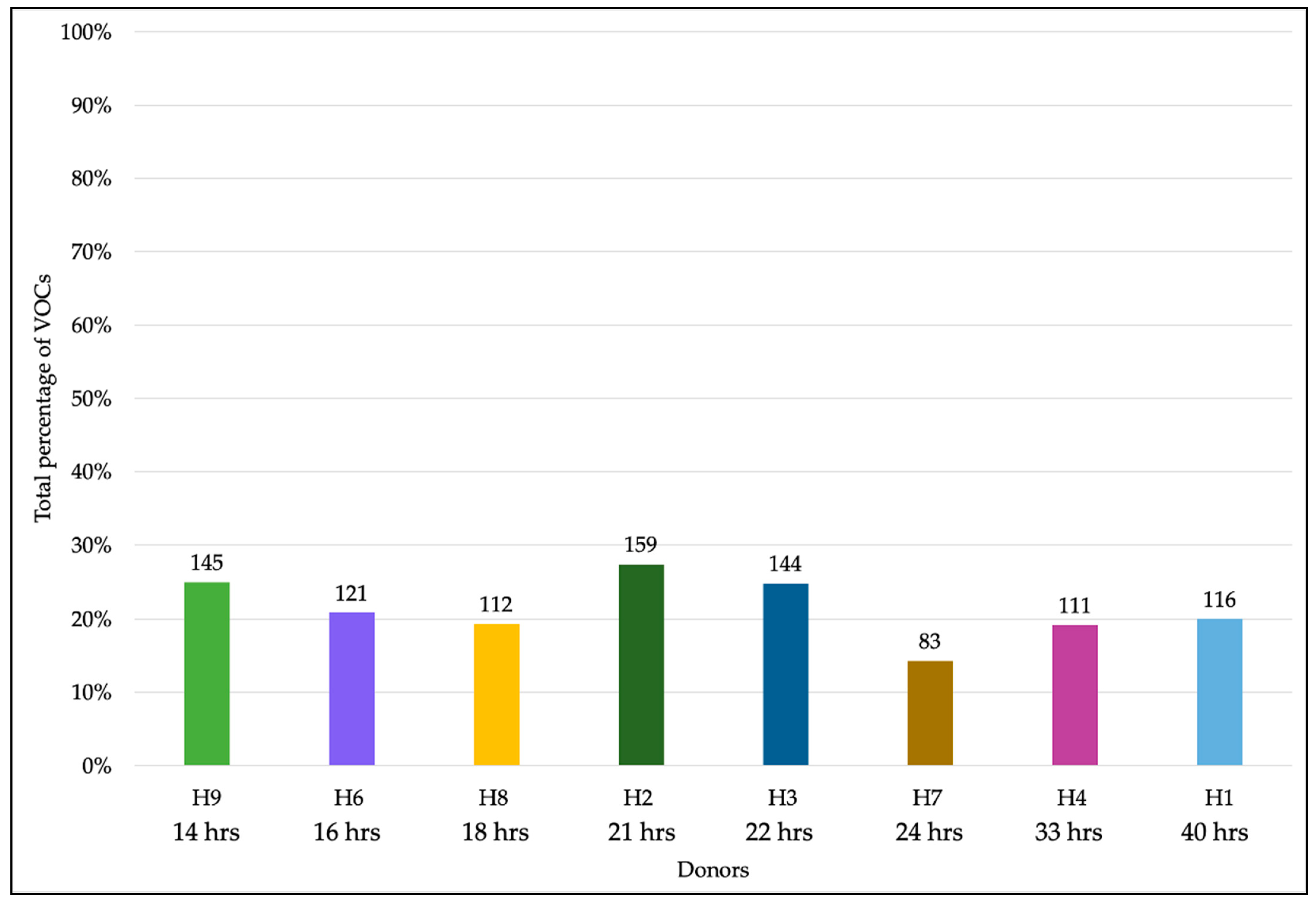
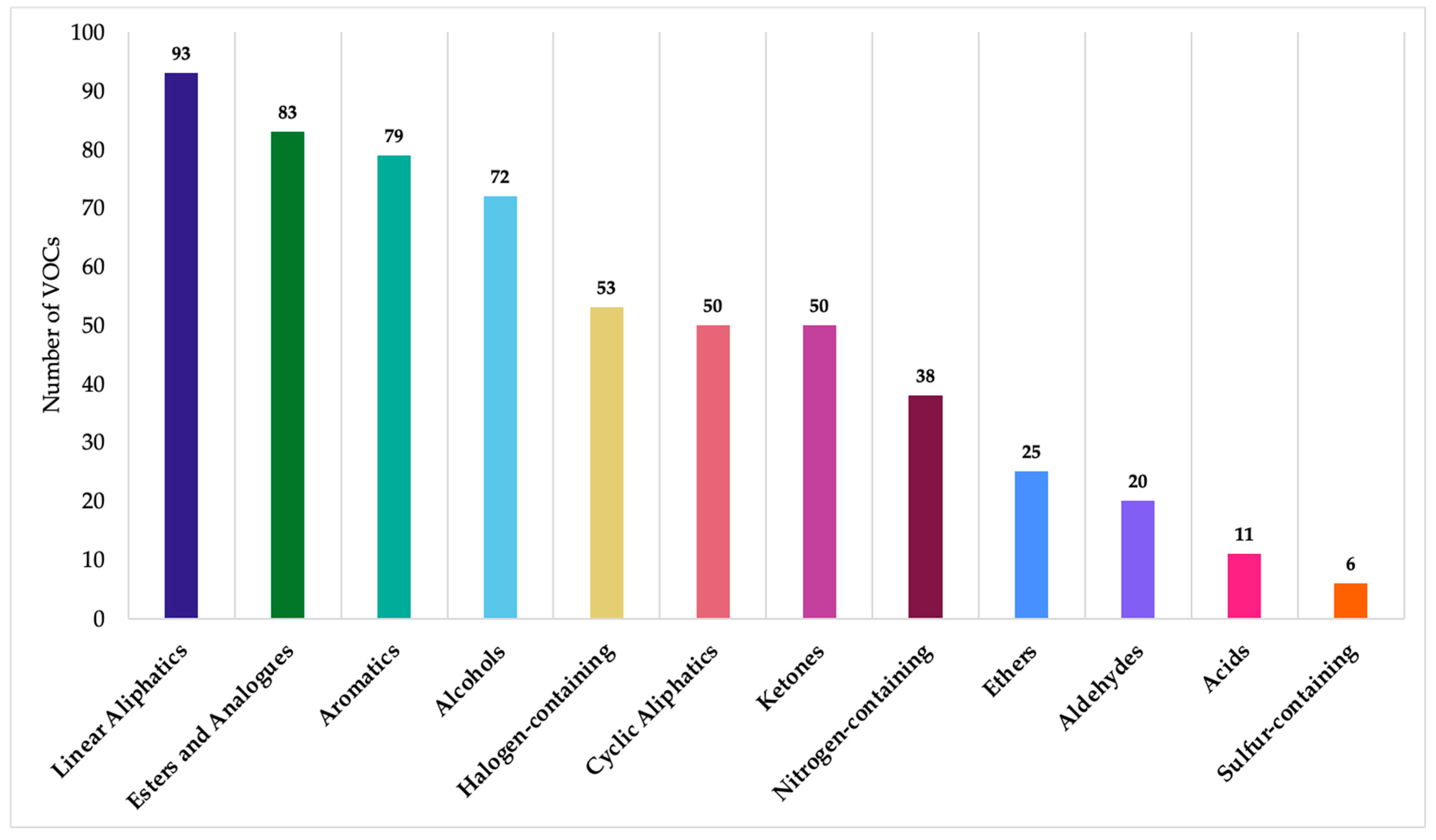
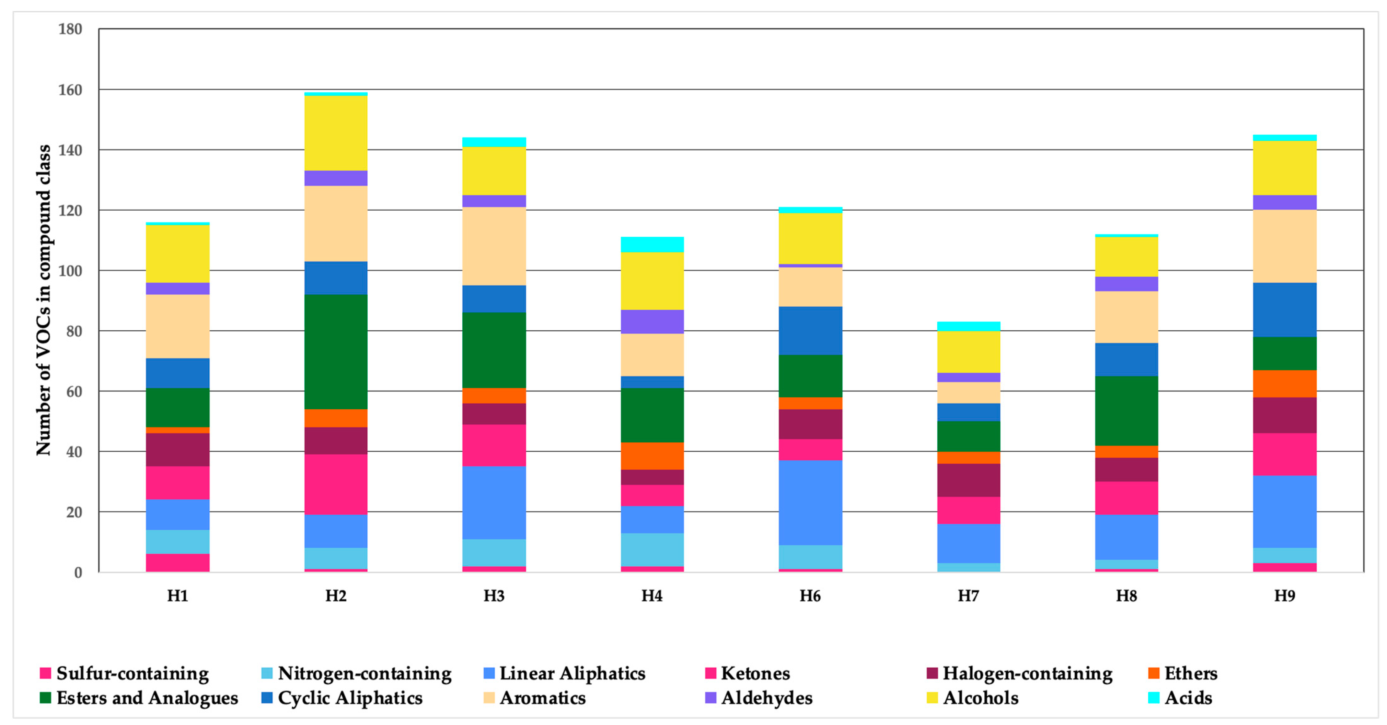
3.1. Overall VOC and Chemical Class Abundance Detected in the Morgue

Across all samples collected from eight donors, a total of 580 VOCs were identified. The differences in the VOC abundances were identified when the VOC abundance of an individual donor was compared with the overall VOC abundance (n = 580 VOCs). The VOC abundance per donor ranged from 83 to 159 and in terms of percentages, 14 to 27% of the total VOCs detected. This difference in the VOC abundance highlights the variation observed in the VOCs between the donors in the same environment at different post-mortem intervals (PMI) (Figure 2).
The VOCs were classified into their chemical class based on the functional groups: alcohols, aldehydes, acids, aromatics, cyclic aliphatic compounds, esters and analogues, ethers, halogen-containing compounds, ketones, linear aliphatic compounds, nitrogen-containing compounds, and sulfur-containing compounds. VOCs identified as anhydride and lactones were classified as analogues in the esters and analogues class. These chemical classes have been previously reported in human decomposition studies conducted in indoor and outdoor scenarios [9,14,24]. The most abundant chemical classes identified in the early post-mortem VOC profiles collected in the morgue were linear aliphatic compounds, esters and analogues, and aromatics, whereas ethers, aldehydes, and sulfur-containing compounds were the least abundant chemical classes (Figure 3).
Across the eight donors, the chemical class with the most abundance varied. Linear aliphatic compounds dominated chemical class abundance in donors H6 and H9, while esters and their analogues were the most abundant chemical class in donors H2 and H4 (Figure 4).
Aromatics and alcohols were the chemical classes that appeared in the greatest abundance for donors H3 and H7. Conversely, for all donors, acids and sulfur-containing compounds were the least prevalent chemical classes identified in the early post-mortem VOC profiles gathered at the morgue (Figure 4). Notably, these chemical classes were not detected in donor H7.
A total of 104 VOCs were detected with a minimum detection frequency of three, which means that these VOCs were detected in a minimum of three donor samples (across all of their replicates) from the eight donors analyzed in this study (thus were present in 38% or more of the samples). All the chemical classes reported in the overall chemical class abundance were identified within these 104 VOCs. Interestingly, two VOCs (propofol and methenamine) related to anesthesia or medication were identified in the headspaces of donors H3 and H4 (Table 1).
This is a new and unexpected finding of this study as the information regarding medications administered to these donors was not shared in their death certificates. These medications were identified in donors H3 and H4, but they were not common between the donors.

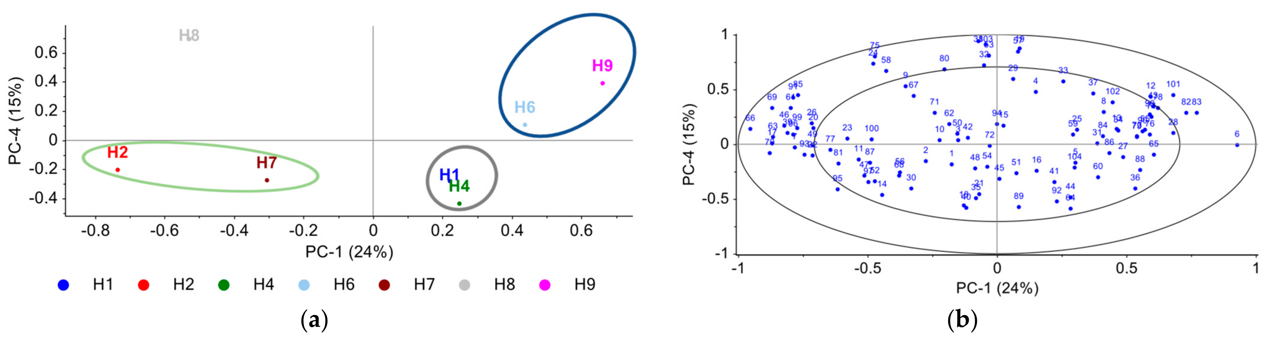
3.2. Principal Component Analysis (PCA)

The compounds for PCA were chosen based on their frequency of detection in multiple donor samples collected at different PMI intervals. Prior to PCA, pre-processing steps included mean centering, standard deviation scaling, and unit vector normalization. Initially, all individual compounds (580 VOCs) having a minimum detection frequency of one out of eight (donors) were used for PCA. Figure 5 shows the PCA constructed from VOC samples collected from eight donors and 580 compounds. PC-1 and PC-2 accounted for 17% and 16% of the explained variance.
Notably, donor H3 which separated along PC-2 contributed to the majority of explained variance among all the donors in the first two principal components, whereas all other donors were separated along PC-1 (Figure 5a). This suggested a large impact from donor H3 on the overall structure of the scores, potentially skewing the data. The loadings plot shows the clustering of compounds along the origin, with these compounds exhibiting the loadings values of less than 0.1, indicating a weak influence on the donor samples (Figure 5b).
Donor H3 was removed from the PCA to further investigate the variance between the other donors. Subsequently, a PCA was carried out on 104 VOCs, chosen based on detection frequency. In this untargeted study, the selection of these VOCs was guided not by statistical measures, but by their detection across varying post-mortem intervals in different donors. This step further facilitated the visualization of the discriminatory information conveyed by the more prevalent analytes identified within the dataset. Figure 6 shows the PCA constructed with 104 compounds identified across seven donors.
Five principal components (PCs) accounted for 88% of the variance in the data, with PC-1 and PC-2 explaining the majority (42%) of this variance. Notably, an interesting clustering pattern that can be correlated to the donors’ PMI can be observed in PC-1 vs. PC-4 (Figure 6a). VOC samples from donors H1 and H4 were collected at a higher PMI (40 and 33 h, respectively), while H9, H6, and H8 were collected at a lower PMI (14, 16, and 18 h, respectively). The VOC samples from donors H2 and H7 were collected at a PMI of 21 and 24 h. Figure 6a shows that the VOC samples collected from donors H1 and H4, at a higher PMI, formed a cluster along PC-4 (highlighted with grey circle), while the VOC samples collected from donors H6 and H9 at a lower PMI were clustered along PC-4 (highlighted with a blue circle). VOC samples collected from H2 and H7 at a PMI of 21 and 24 h made a cluster along PC-1 (highlighted with a green circle), while VOC samples collected from H8 at a PMI interval of 18 h were separated from the rest of the donors along PC-4 (Figure 6a). The distribution of compounds in the correlation loadings highlighted potential VOCs associated with the corresponding donors (Figure 6b). The analytes present inside the region defined by the two ellipses indicate how much variance is considered by the PCA model (100% and 50% for the outer and inner ellipses, respectively). The compounds presenting closest to the outer ring showed a strong association to the donor samples and are listed in Table S2. The correlation loadings plot did not show a strong association of compounds with the corresponding donors H1 and H4. Therefore, the PCAs were also performed using compound classes to investigate their influence on VOC profiles.
Figure 7 shows a biplot of the scores and loadings made up of compound classes for the donors. For each compound class in the loadings, normalized peak areas were summed.
Overall variability can be observed in the correlation of compound classes with donors (Figure 7). Notably, sulfur-containing compounds were positively correlated with the donors (H1 and H4) that had higher PMI (40 and 33 h), whereas donor H8 with a PMI of 18 h was positively correlated with compound classes such as aldehydes, ketones, and ethers (Figure 7).

4. Discussion

4.1. Overall VOC and Chemical Class Abundance Detected in the Morgue Donor Samples

During the early post-mortem period, the number of VOCs and the chemical class abundance varied (Figure 3 and Figure 4). These variations can be linked with intrinsic factors such as donor age, sex, BMI, physiology, biochemistry, and pathophysiology [27]. Additionally, the variations in the chemical class abundance are indicative of these donor-to-donor variations, which can affect the decomposition process. Different VOC classes linked with complex biochemical processes occurring during life are detected, indicating the persistence of the living scent during the early post-mortem period. Notably, this variability was not reported in the studies previously conducted in the morgue [23,28]. The sample size of the study, ethical challenges, and restrictions for the use of donors for studying decomposition could possibly explain the lack of reporting as these studies were conducted on only one or two donors. To date, there has only been one study with a large donor sample set (n = 21) conducted in the morgue [14]. The authors of this study focused on differentiating between the live, deceased, and animal scent, and thus the class abundance of an individual donor was not the focus of the study. Furthermore, the authors were focused on highlighting the potential application of this novel sample collection technique to identify key compounds related to the decomposition process. In contrast, variation in the number of VOCs among donors has been reported in decomposition studies conducted in an outdoor environment [9,16]. The application of comprehensive GC×GC-TOFMS is the common aspect between the current study and the other studies [9,16]. Further, this instrument allows the separation of complex VOCs present in the decomposition odor, allowing for its characterization.
Compound classes such as esters and analogues and linear aliphatic compounds were the most abundant classes detected in the current study. The generation of these classes of VOCs has been linked with the breakdown of fatty acids and carbohydrates during the post-mortem period [4,29,30]. These compound classes have also been detected in the VOC samples collected from skin and are produced due to the interaction of the microbiomes on the surface of the skin and with skin components (sweat, amino acids, sebum) [31,32]. However, the production of VOCs from the surface of the skin is dependent on factors such as the pathology and physiology of an individual. Therefore, during the early post-mortem period, the VOC profile could consist of VOCs which are linked to both post-mortem and ante-mortem odor, making it challenging to characterize.
The 104 compounds were chosen based on their minimum detection frequency accounting for their identification in 38% of the samples collected. Out of these 104 compounds, 8 have been previously reported in the headspace of human scent studies, urine, or in skin. The details of these compounds are provided in Table 2.
In this study, 19 VOCs that have been previously detected in human decomposition studies conducted on human remains or human donors were identified (Table 3). Their identification suggests that during the transition from ante-mortem odor to post-mortem odor, VOCs associated with the human decomposition process can be detected during the early post-mortem period. Further, the headspace analysis of VOCs from the donors in the morgue environment can lead to the identification of VOCs linked with the decomposition process. Although the abundance may vary, this analysis can provide a baseline VOC profile of a person soon after death. The morgue studies conducted by Statheropoulos et al. [28] and DeGreeff et al. [14] also reported VOCs related to decomposition processes, such as DMTS and DMDS, which were detected in the early post-mortem period in a morgue scenario. This study supports the findings from these previous studies [28].

4.2. Principal Component Analysis

Initially, PCA was conducted with 580 compounds identified in all donors. PC-1 and PC-2 accounted for 33% of the overall variance. The separation of donors along PC-1 and PC-2 highlighted variance in the VOC profiles between these donors. Donor H3 was separated from all other donors along PC-2, which explained 16% of the variance, and this separation of donor H3 indicated that it had a different VOC profile compared to the other donors. Intrinsic factors such as biological, physiological, and pathophysiological variation might have led to differences in the VOC profile of donor H3 during the early post-mortem period [46,47]. The loadings value of 580 compounds identified across all the donors was low (less than 0.1), suggesting that several compounds within these 580 compounds had a weak association with the donors present in the scores plot. Among the 580 compounds, ~60% of the compounds were identified with a detection frequency of one out of eight, indicating that these compounds had lower significance and might not strongly associate with all the donors in the scores plot contributing to their variances [47]. Thus, these low-detection compounds which were identified in less than three donor samples were removed from the PCA as they did not provide any donor-specific information. Stefanuto et al. [8] reported a similar finding from PCA based on matrices of data containing 1200 individual compounds identified in the study [47]. However, using all 1200 compounds for PCA provided no valuable information that can highlight the identification of compounds specific to the early post-mortem VOC profile. Thus, other PCAs were constructed with compounds identified at a higher minimum detection frequency of three out of eight donor samples, which reduced the dataset to 104 compounds. This cut-off, three of eight, was chosen heuristically based on compound quantity reduction.
The PCA, constructed with all the donors except donor H3, showed a noteworthy pattern of clustering and separation in the scores plot made up of VOC samples collected from seven donors. This clustering and separation pattern can be correlated to the PMI at which these samples were collected. The clustering of the VOC samples collected at different PMI intervals indicates a common suite of VOCs appearing at certain PMI, which can be expected across donors. The separation of VOC samples collected at different PMI intervals highlights the dynamic nature of VOC profiles released during the early post-mortem period. Moreover, it also highlights the fact that the decomposition process is not a single event but a continuous process [23,47].
The correlation plots and loadings plot of 104 compounds were used to Identify the association of VOCs responsible for causing these patterns in the scores plot. The loadings plot highlighted the subtle influences of the VOCs, contributing to the separation and clustering of these donors. For donors with higher PMI (H4 and H1), no VOCs in the correlation loadings showed a strong association [47]. VOCs previously reported in the decomposition literature were identified in the samples of donors H8, H9, H6, H2, and H7, which were collected at a lower PMI (Table S2). These decomposition-related VOCs were closest to the outer ring of the correlation loadings, indicating a strong association with these VOC samples and further contributing to the variances in the VOC sample collected at a lower PMI. Thus, the presence of decomposition-related VOCs in these donors indicates the change in the VOC profile as early as 14 h PMI. This finding can be useful in the context of search and rescue operations and HRD dog training. Furthermore, the PCAs were able to highlight and support the fact that even in a controlled environment, VOC profiles released during the early post-mortem period can change hourly, and these changes can be driven by VOCs related to the decomposition process. Further studies are required with similar instrumentation and methodology which would allow a direct data comparison and help us to build a dataset of VOCs which are present consistently in the early post-mortem period.
The biplot was constructed with scores plots consisting of VOC samples collected from seven donors and loadings showing 104 compounds classified into their compound class. The normalized areas for each compound within the list of 104 compounds were summed for each class. The biplot highlighted the correlation of different compound classes contributing to the variance in the VOC profiles of the donors in the early post-mortem period. Overall variability can be observed in the compound classes contributing to the variance in the donor profiles. Therefore, no single compound class strongly influences the VOC profiles across all donors during the early post-mortem period. This result supports the findings of an outdoor study conducted by Deo et al. [16], whereby a similar variability was observed in the donor VOC profiles collected across different donors and seasons.
Notably, sulfur-containing compounds were identified to be positively correlated to the donors H1 and H4, whose samples were collected at a higher PMI. Sulfur-containing compounds are produced due to the breakdown of proteins and are linked to bacterial activity. Thus, the identification of the sulfur-containing compounds can be correlated with the progression of the decomposition for these donors. In the case of donor H1, this positive correlation can be further supported by macroscopic changes such as greenish discoloration and venous marbling associated with the progression of the decomposition process during the early post-mortem period.

4.3. Limitations

Research on decomposition VOCs conducted with donors presents ethical and logistical challenges. These challenges introduce limitations and biases in the experimental design. In this study, limitations were presented in terms of limited control over the storage and transport of donors before arriving at the UQTR morgue facility. It is important to note that inherent sample-to-sample variation exists, as no two human beings are identical. This presents limitations in method optimization as sample-to-sample variation will exceed method-to-method variation. Potential experimental design biases in this study arise from the conscious effort to facilitate comparisons with previously conducted research. The experimental parameters, specifically the use of stainless-steel dual sorbent tubes, column combinations, modulation period, and normalization procedures, have been reported to be suitable for decomposition VOC analysis. For the current study, since other sample collection methods such as SPME or normalization procedures were not assessed, there may have been a bias introduced when establishing the study design.

5. Conclusions

Profiling VOCs from donors in indoor and outdoor environments during the early post-mortem period is an analytical challenge due to the low VOC abundance. In the present study, the experimental design and analytical method aided in the collection of the VOCs and investigation of the VOC profile released from the donors in the controlled environment (morgue) within a 6–72 h post-mortem period. The early post-mortem VOC profiles of the donors were identified to be complex immediately after death. These VOC profiles comprised different chemical classes identified at varying abundances. Moreover, several VOCs previously identified in the middle and later stages of the decomposition process were also identified in the VOC profiles of the donors between 14–40 h PMI. Their identification suggests that VOCs related to the decomposition process can be detected as early as 14–40 h PMI. Additionally, non-decomposition VOCs related to skin, donor medications, and biomarkers related to pathologies were also detected, highlighting the potential of this technique to be applied in forensic pathology and toxicology as a non-destructive approach to sample analysis. Furthermore, increasing the number of donors in future studies can aid in identifying the correlations of VOC abundance with the PMI interval and effects of refrigeration. A larger sample size would aid in building a database of VOCs that can consistently be detected during the early post-mortem period and act as biomarkers linked with the early post-mortem VOC profile.

Supplementary Materials

The following supporting information can be downloaded at https://www.mdpi.com/article/10.3390/separations10110566/s1, Figure S1: GC×GC-TOFMS total ion current (TIC) contour plots of headspace VOC samples collected from donors H1, H2, H3 and H4; Figure S2: GC×GC-TOFMS total ion current (TIC) contour plots of headspace VOC samples collected from donors H6, H7, H8 and H9; Table S1: Decomposition standard compounds analyzed and their retention times using the cur-rent optimized stage 2 method and instrumentation. Note: over the course of the study, the major peaks of all the standards appeared within ± 5 s in 1D and ± 0.1 s in 2D from the retention values listed below; Table S2: List of compounds related to decomposition identified in lower PMI donors causing their sepa-ration and clustering in the scores plot made with seven donors. These compounds were located closest to the outer ellipses on the correlations loadings plot indicating a strong association and correlation with the donors causing variance in the VOC profiles.

Author Contributions

Conceptualization, D.P. and S.F.; Data Curation, D.P. and W.S.B.; Formal analysis, D.P.; Funding acquisition, S.F.; Investigation, D.P. and R.D.; Methodology, D.P. and S.F.; Project Administration, D.P. and S.F.; Resources, W.S.B. and S.F.; Software, D.P. and W.S.B.; Development of R functions and R code for analysis, W.S.B.; Supervision, B.D. and S.F.; Validation, D.P., R.D. and B.D.; Visualization D.P., R.D. and W.S.B.; Writing—original draft D.P.; Writing—review and editing, D.P., R.D., W.S.B., B.D. and S.F. All authors have read and agreed to the published version of the manuscript.

Funding

The Canada 150 Research Chair in Forensic Thanatology [C150-2017-12] and the Natural Sciences and Engineering Research Council of Canada [RGPIN/6098/2019] supported this research.

Institutional Review Board Statement

The cadavers used in this study were donated through the UQTR Body Donation Program, which includes consent for the remains to be used for the purpose of research at the UQTR morgue. This project was approved by the UQTR Human Research Ethics Committee (CER-19-261-07.11) and Sous-comité d’éthique du laboratoire d’enseignement et de la recherche en anatomie (SCELERA), certificate number SCELERA- 20-09 approved on 11 June 2020. The cadavers were transported to the UQTR morgue by funeral directors licensed to transport human remains.

Data Availability Statement

The data presented in this study are available on request from the corresponding author. The R programming script developed for the data analysis can be found in following repository https://github.com/wesleyburr/GCxGC_Morgue_RESTES (accessed on 30 October 2023).

Conflicts of Interest

The authors declare no conflict of interest.

References

  1. Stuart, B. Decomposition chemistry: Overview, analysis, and interpretation. In Encyclopedia of Forensic Sciences; Elsevier: Amsterdam, The Netherlands, 2013; Volume 2, pp. 11–15. [Google Scholar]
  2. Forbes, S.L.; Perrault, K.A.; Comstock, J.L. Microscopic post-mortem changes: The chemistry of decomposition. In Taphonomy of Human Remains: Forensic Analysis of the Dead and the Depositional Environment; Wiley Online Library: Hoboken, NJ, USA, 2017; pp. 26–38. [Google Scholar]
  3. Knight, B. Forensic Pathology; Oxford University Press: Oxford, UK, 1991. [Google Scholar]
  4. Dent, B.B.; Forbes, S.L.; Stuart, B.H. Review of human decomposition processes in soil. Environ. Geol. 2004, 45, 576–585. [Google Scholar] [CrossRef]
  5. Clark, M.A.; Worrell, M.B.; Pless, J.E. Postmortem changes in soft tissues. Forensic Taphon. Postmortem Fate Hum. Remain. 1997, 151–164. [Google Scholar]
  6. Vass, A.A.; Barshick, S.-A.; Sega, G.; Caton, J.; Skeen, J.T.; Love, J.C.; Synstelien, J.A. Decomposition chemistry of human remains: A new methodology for determining the postmortem interval. J. Forensic Sci. 2002, 47, 542–553. [Google Scholar] [CrossRef] [PubMed]
  7. Forbes, S.L.; Perrault, K.A.; Stefanuto, P.-H.; Nizio, K.D.; Focant, J.-F. Comparison of the decomposition VOC profile during winter and summer in a moist, mid-latitude (Cfb) climate. PLoS ONE 2014, 9, e113681. [Google Scholar] [CrossRef] [PubMed]
  8. Stefanuto, P.-H.; Perrault, K.A.; Stadler, S.; Pesesse, R.; LeBlanc, H.N.; Forbes, S.L.; Focant, J.-F. GC × GC–TOFMS and supervised multivariate approaches to study human cadaveric decomposition olfactive signatures. Anal. Bioanal. Chem. 2015, 407, 4767–4778. [Google Scholar] [CrossRef]
  9. Knobel, Z.; Ueland, M.; Nizio, K.D.; Patel, D.; Forbes, S.L. A comparison of human and pig decomposition rates and odour profiles in an Australian environment. Aust. J. Forensic Sci. 2019, 51, 557–572. [Google Scholar] [CrossRef]
  10. Mochalski, P.; Unterkofler, K.; Teschl, G.; Amann, A. Potential of volatile organic compounds as markers of entrapped humans for use in urban search-and-rescue operations. TrAC Trends Anal. Chem. 2015, 68, 88–106. [Google Scholar] [CrossRef]
  11. Agapiou, A.; Amann, A.; Mochalski, P.; Statheropoulos, M.; Thomas, C.L.P. Trace detection of endogenous human volatile organic compounds for search, rescue and emergency applications. TrAC Trends Anal. Chem. 2015, 66, 158–175. [Google Scholar] [CrossRef]
  12. Armstrong, P.; Nizio, K.D.; Perrault, K.A.; Forbes, S.L. Establishing the volatile profile of pig carcasses as analogues for human decomposition during the early postmortem period. Heliyon 2016, 2, e00070. [Google Scholar] [CrossRef]
  13. Tsokos, M. Forensic Pathology Reviews; Springer: Berlin/Heidelberg, Germany, 2007; Volume 4. [Google Scholar]
  14. DeGreeff, L.E.; Furton, K.G. Collection and identification of human remains volatiles by non-contact, dynamic airflow sampling and SPME-GC/MS using various sorbent materials. Anal. Bioanal. Chem. 2011, 401, 1295–1307. [Google Scholar] [CrossRef]
  15. Stadler, S.; Stefanuto, P.-H.; Brokl, M.; Forbes, S.L.; Focant, J.-F. Characterization of volatile organic compounds from human analogue decomposition using thermal desorption coupled to comprehensive two-dimensional gas chromatography–time-of-flight mass spectrometry. Anal. Chem. 2013, 85, 998–1005. [Google Scholar] [CrossRef]
  16. Deo, A.; Forbes, S.L.; Stuart, B.H.; Ueland, M. Profiling the seasonal variability of decomposition odour from human remains in a temperate Australian environment. Aust. J. Forensic Sci. 2020, 52, 654–664. [Google Scholar] [CrossRef]
  17. Ueland, M.; Harris, S.; Forbes, S.L. Detecting volatile organic compounds to locate human remains in a simulated collapsed building. Forensic Sci. Int. 2021, 323, 110781. [Google Scholar] [CrossRef] [PubMed]
  18. Perrault, K.A.; Nizio, K.D.; Forbes, S.L. A Comparison of One-Dimensional and Comprehensive Two-Dimensional Gas Chromatography for Decomposition Odour Profiling Using Inter-Year Replicate Field Trials. Chromatographia 2015, 78, 1057–1070. [Google Scholar] [CrossRef]
  19. Stefanuto, P.H.; Rosier, E.; Tytgat, J.; Focant, J.F.; Cuypers, E. Profiling volatile organic compounds of decomposition. In Taphonomy of Human Remains: Forensic Analysis of the Dead and the Depositional Environment:Forensic Analysis of the Dead and the Depositional Environment; Wiley Online Library: Hoboken, NJ, USA, 2017; pp. 39–52. [Google Scholar]
  20. Nizio, K.D.; Cochran, J.W.; Forbes, S.L. Achieving a Near-Theoretical Maximum in Peak Capacity Gain for the Forensic Analysis of Ignitable Liquids Using GC×GC-TOFMS. Separations 2016, 3, 26. [Google Scholar] [CrossRef]
  21. Ramos, L. Comprehensive Two Dimensional Gas Chromatography; Elsevier: Amsterdam, The Netherlands, 2009. [Google Scholar]
  22. Woolfenden, E.; McClenny, W. Compendium Method TO-17. In Determination of Volatile Organic Compounds in Ambient Air Using Active Sampling Onto Sorbent Tubes; US EPA: Cincinnati, OH, USA, 1999. [Google Scholar]
  23. Statheropoulos, M.; Spiliopoulou, C.; Agapiou, A. A study of volatile organic compounds evolved from the decaying human body. Forensic Sci. Int. 2005, 153, 147–155. [Google Scholar] [CrossRef] [PubMed]
  24. Statheropoulos, M.; Agapiou, A.; Pallis, G. A study of volatile organic compounds evolved in urban waste disposal bins. Atmos. Environ. 2005, 39, 4639–4645. [Google Scholar] [CrossRef]
  25. McKeage, K.; Perry, C.M. Propofol. CNS Drugs 2003, 17, 235–272. [Google Scholar] [CrossRef]
  26. Lo, T.S.; Hammer, K.D.P.; Zegarra, M.; Cho, W.C.S. Methenamine: A forgotten drug for preventing recurrent urinary tract infection in a multidrug resistance era. Expert Rev. Anti-Infect. Ther. 2014, 12, 549–554. [Google Scholar] [CrossRef]
  27. Zhou, C.; Byard, R.W. Factors and processes causing accelerated decomposition in human cadavers–an overview. J. Forensic Leg. Med. 2011, 18, 6–9. [Google Scholar] [CrossRef]
  28. Statheropoulos, M.; Agapiou, A.; Spiliopoulou, C.; Pallis, G.C.; Sianos, E. Environmental aspects of VOCs evolved in the early stages of human decomposition. Sci. Total Environ. 2007, 385, 221–227. [Google Scholar] [CrossRef]
  29. Boumba, V.A.; Ziavrou, K.S.; Vougiouklakis, T. Biochemical pathways generating post-mortem volatile compounds co-detected during forensic ethanol analyses. Forensic Sci. Int. 2008, 174, 133–151. [Google Scholar] [CrossRef]
  30. Paczkowski, S.; Schütz, S. Post-mortem volatiles of vertebrate tissue. Appl. Microbiol. Biotechnol. 2011, 91, 917–935. [Google Scholar] [CrossRef]
  31. Mochalski, P.; King, J.; Unterkofler, K.; Hinterhuber, H.; Amann, A. Emission rates of selected volatile organic compounds from skin of healthy volunteers. J. Chromatogr. B Analyt. Technol. Biomed. Life Sci. 2014, 959, 62–70. [Google Scholar] [CrossRef] [PubMed]
  32. Jiang, R.; Cudjoe, E.; Bojko, B.; Abaffy, T.; Pawliszyn, J. A non-invasive method for in vivo skin volatile compounds sampling. Anal. Chim. Acta 2013, 804, 111–119. [Google Scholar] [CrossRef] [PubMed]
  33. Rust, L.; Nizio, K.D.; Forbes, S.L. The influence of ageing and surface type on the odour profile of blood-detection dog training aids. Anal. Bioanal. Chem. 2016, 408, 6349–6360. [Google Scholar] [CrossRef]
  34. Gallagher, M.; Wysocki, C.J.; Leyden, J.J.; Spielman, A.I.; Sun, X.; Preti, G. Analyses of volatile organic compounds from human skin. Br. J. Dermatol. 2008, 159, 780–791. [Google Scholar] [CrossRef]
  35. Dormont, L.; Bessière, J.-M.; McKey, D.; Cohuet, A. New methods for field collection of human skin volatiles and perspectives for their application in the chemical ecology of human–pathogen–vector interactions. J. Exp. Biol. 2013, 216, 2783–2788. [Google Scholar] [CrossRef]
  36. Penn, D.J.; Oberzaucher, E.; Grammer, K.; Fischer, G.; Soini, H.A.; Wiesler, D.; Novotny, M.V.; Dixon, S.J.; Xu, Y.; Brereton, R.G. Individual and gender fingerprints in human body odour. J. R. Soc. Interface 2007, 4, 331–340. [Google Scholar] [CrossRef] [PubMed]
  37. Curran, A.M.; Rabin, S.I.; Prada, P.A.; Furton, K.G. Comparison of the volatile organic compounds present in human odour using SPME-GC/MS. J. Chem. Ecol. 2005, 31, 1607–1619. [Google Scholar] [CrossRef] [PubMed]
  38. Shirasu, M.; Touhara, K. The scent of disease: Volatile organic compounds of the human body related to disease and disorder. J. Biochem. 2011, 150, 257–266. [Google Scholar] [CrossRef]
  39. Rosier, E.; Loix, S.; Develter, W.; Van de Voorde, W.; Tytgat, J.; Cuypers, E. The search for a volatile human specific marker in the decomposition process. PLoS ONE 2015, 10, e0137341. [Google Scholar] [CrossRef] [PubMed]
  40. Vass, A.A.; Smith, R.R.; Thompson, C.V.; Burnett, M.N.; Wolf, D.A.; Synstelien, J.A.; Dulgerian, N.; Eckenrode, B.A. Decompositional odor analysis database. J. Forensic Sci. 2004, 49, 760–769. [Google Scholar] [CrossRef]
  41. Vass, A.A. Odor mortis. Forensic Sci. Int. 2012, 222, 234–241. [Google Scholar] [CrossRef] [PubMed]
  42. Hoffman, E.M.; Curran, A.M.; Dulgerian, N.; Stockham, R.A.; Eckenrode, B.A. Characterization of the volatile organic compounds present in the headspace of decomposing human remains. Forensic Sci. Int. 2009, 186, 6–13. [Google Scholar] [CrossRef] [PubMed]
  43. Trumbo, S.T.; Steiger, S. Finding a fresh carcass: Bacterially derived volatiles and burying beetle search success. Chemoecology 2020, 30, 287–296. [Google Scholar] [CrossRef]
  44. Martin, C.; Verheggen, F. Odour profile of human corpses: A review. Forensic Chem. 2018, 10, 27–36. [Google Scholar] [CrossRef]
  45. Dargan, R.; Samson, C.; Burr, W.S.; Daoust, B.; Forbes, S.L. Validating the Use of Amputated Limbs Used as Cadaver Detection Dog Training Aids. Front. Anal. Sci. 2022, 2, 934639. [Google Scholar] [CrossRef]
  46. Wescott, D.J. Recent Advances in Forensic Anthropology: Decomposition Research. Forensic Sci. Res. 2018, 3, 278–293. [Google Scholar] [CrossRef] [PubMed]
  47. Patel, D. Identifying the Transition from Ante-Mortem Odour to Post-Mortem Odour Traditional; Université du Québec à Trois-Rivières: Québec, QC, Canada, 2023. [Google Scholar]
Figure 1. Sample collection method from donors in the UQTR morgue using the ACTI-VOC low flow pump and sorbent tube.
Separations 10 00566 g001
Figure 2. Percentage difference observed at 14 to 40 h PMI between the number of VOCs of an individual donor vs. the total VOCs identified in all eight donor samples (Note: PMIs are approximate time values and shown in increasing order).
Separations 10 00566 g002
Figure 3. Number of VOCs identified by chemical class (high to low) in the morgue study from all eight donors.
Separations 10 00566 g003
Figure 4. VOC chemical class distribution per donor identified during the early post-mortem period in the morgue study.
Separations 10 00566 g004
Figure 5. PCA showing (a) scores plot and (b) loadings plot calculated using pre-processed GC×GC TOFMS data of 580 compounds identified across all eight donors. Donor H3 was separated along PC-2 from all other donors along PC-2. The loadings plot shows the distribution of compounds along PC-1 and PC-2 with compounds having a value less than 0.1 indicating weak association with the donors present in the scores plot.
Separations 10 00566 g005
Figure 6. PCA (a) scores plot and (b) correlation loadings plot for PC-1 vs. PC-4. PCA were calculated using pre-processed GC×GC-TOFMS normalized peak areas of 104 compounds identified with a minimum detection frequency of three out of eight. The scores plot of PC-1 vs. PC-4 shows separation and clustering of donor samples collected at different PMI intervals. Here, blue circles represent donor samples (H9 and H6) collected at lower PMI (14 and 16 h), grey circles highlight donor samples (H1 and H4) collected at higher PMI (40 and 33 h), and green circles highlight donor samples (H2 and H7) collected at PMI of 21 and 24 h. The correlation plots highlight VOCs contributing to the variances in the donor VOC profiles.
Separations 10 00566 g006
Figure 7. Biplot of donors and compound classes, showing PCA scores and loadings calculated using donor and compound class data. Each compound class represents the sum of all the normalized peak areas of its constituent compounds.
Separations 10 00566 g007
Table 1. List of VOCs related to medications identified in the headspace of the body bags containing donors in the morgue study.
DonorsVOCsChemical ClassUsesReferences
H3PropofolAlcoholInhalation and intravenous anesthetic[25]
H4MethenamineNitrogen-containing compoundAntibacterial (urinary tract infection)[26]
Table 2. The frequency of detection, percentage abundance, sources of release, and citation in previous studies of 8 VOCs among the top 104 identified in donors in the morgue.
VOCFrequency (Out of 8 Donors)Percentage Abundance (%) Potential SourcesPreviously Reported in the Literature
6-methylhept-5-en-2-one737.5Human scent study[33]
Acetic acid, butyl ester562.5Skin[34]
Benzyl alcohol337.5Skin[35]
Decanoic acid, ethyl ester337.5Skin[31]
Hexanoic acid, methyl ester450Skin[36]
1,3-Dioxolane, 2-methyl-337.5Skin[14,37]
2,3-Pentanedione562.5Skin (axillary skin)/sweat[38]
1-Octen-3-one450Urine[14]
Table 3. The frequency of detection, percentage abundance, and citation in previous studies of 19 VOCs among the most prevalent 104 VOCs identified in donors in the morgue.
VOCFrequency (Out of 8 Donors)Percentage
Abundance (%)
Previously Reported in the Literature
3-methyl-1-butanol676[39]
2-Pentanol450[39]
Octanoic acid, ethyl ester450[14,40]
Furan, 2-pentyl-337.5[41]
3-methylbutanal450[28]
Pyridine450[39]
Dimethyl disulfide562.5[23,28,39,40]
Dimethyl sulfone450[14]
1,2-propanediol 337.5[41]
Butanoic acid, 3-methyl337.5[39]
2-Octenal337.5[42]
Heptane,2-4 dimethyl337.5[28]
Thiocyanic acid, methyl ester337.5[43]
Butanal, 3-methyl562.5[28]
Terpineol337.5[33]
2-Propenoic acid, butyl ester362.5[44]
Butanenitrile337.5[8,45]
Butanenitrile 3-methyl337.5[45]
2-pentanol437.5[44]
Disclaimer/Publisher’s Note: The statements, opinions and data contained in all publications are solely those of the individual author(s) and contributor(s) and not of MDPI and/or the editor(s). MDPI and/or the editor(s) disclaim responsibility for any injury to people or property resulting from any ideas, methods, instructions or products referred to in the content.

