
Multidimensional Fractionation of Particles
by
 ,
,
Uwe Frank
1, 
Jana Dienstbier
2,
Florentin Tischer
1,
Simon E. Wawra
1,
Lukas Gromotka
1,
Johannes Walter
1,3,
Frauke Liers
2 and
Wolfgang Peukert
1,3,* 1
Institute of Particle Technology, Friedrich-Alexander-Universität Erlangen-Nürnberg, Cauerstraße 4, D-91058 Erlangen, Germany
2
Department of Data Science (DDS), Optimization under Uncertainty & Data Analysis, Friedrich-Alexander-Universität Erlangen-Nürnberg, Cauerstraße 11, D-91058 Erlangen, Germany
3
Center for Functional Particle Systems, Friedrich-Alexander-Universität Erlangen-Nürnberg, Haberstraße 9a, D-91058 Erlangen, Germany
*
Author to whom correspondence should be addressed.
Separations 2023, 10(4), 252; https://doi.org/10.3390/separations10040252
Submission received: 14 March 2023
/
Revised: 29 March 2023
/
Accepted: 6 April 2023
/
Published: 13 April 2023
Abstract
:The increasing complexity in particle science and technology requires the ability to deal with multidimensional property distributions. We present the theoretical background for multidimensional fractionations by transferring the concepts known from one dimensional to higher dimensional separations. Particles in fluids are separated by acting forces or velocities, which are commonly induces by external fields, e.g., gravitational, centrifugal or electro-magnetic fields. In addition, short-range force fields induced by particle interactions can be employed for fractionation. In this special case, nanoparticle chromatography is a recent example. The framework for handling and characterizing multidimensional separation processes acting on multidimensional particle size distributions is presented. Illustrative examples for technical realizations are given for shape-selective separation in a hydrocyclone and for density-selective separation in a disc separator.
1. Introduction
Particle science and technology evolve towards ever increasing complexity with respect to multidimensional particle properties. In general, the properties of particle systems can be defined by a five-dimensional parameter space, given as particle size, shape, surface, structure (e.g., pore size, shape or defect distributions) and composition [1]. In the past, our activities were focused mostly on controlling the particle size of a specific material in a wide size regime depending on the application. With the advent of powerful synthesis protocols within nanotechnology, in particular in the liquid phase, narrowly distributed samples first became available. Particle shape, very prominently exemplified by the discovery of 2D materials (e.g., graphene [2,3], MoS2, BN and many other materials), came into focus later. Additionally, complex structures were developed, such as core-shell particles for controlled drug release, quantum dots for optimized electronic properties and metal particles with many other shapes (e.g., rods, tetrapods, double pyramids) showing distinct plasmonic features, as well as nanostructured patchy particles [4]. Particle composition is another variable and includes today not only many one- and two-component systems, but also three- and four-component semiconducting chalcopyrates (e.g., CuInS [5], kesterites such as Cu2ZnSnS4 [6] or battery materials such as NiCoAl or NiCoMg oxides [7]) and even five and more components in minerals and high entropy alloys contained in one single particle. Scaling up from small well-controlled lab syntheses to the industrial scale inevitably leads to a broadening of all property distributions. Many lab protocols and industrial particle-formation processes include steps for purification, phase separation and size classification. In nanotechnology in particular, post-processing is critical and often prohibitive for the transfer from lab scale to industrial production.
The size classification of particles is well established in industry only for particle diameters larger than 1 µm. Typical realizations are impeller wheel classifiers, centrifuges and cyclones. The size separation of nanoparticles is still challenging but recent developments have shown considerable progress. For instance, Nirschl and co-workers demonstrated cut sizes down to a few 10 nm in a discontinuously operated bowl centrifuge [8]. Other examples include strong centrifugal fields in analytical centrifuges [9], electric fields [10,11,12] or size-selective precipitation [13]. Highly promising results were obtained by nanoparticle chromatography both for the purification of complex mixtures, e.g., carbon nanodots [14], single-walled carbon nanotubes [15] and also the classification of plasmonic noble metals and quantum dots [16,17]. Material dependent separations with respect to density, electric or magnetic properties are mostly applied to larger particles, especially in recycling processes. Industrial shape separation is rarely reported in the open literature, whereas protocols for the separation of 2D materials such as nanosheets are promising at lab scale [18]. A national priority program in Germany (PP2045—Highly specific and multidimensional fractionation of particle systems with technical relevance) comprises several projects aiming for multidimensional size, shape and property fractionation [19].
The development of multidimensional separation processes strongly relies on methodologies for the multidimensional characterization of the complex particles. The tedious counting of particles by microscopy strongly limits fast and efficient analysis, which is essential for parameter studies and validation. Interestingly, several new characterization methods beyond size have been developed in the last few years; see a recent review [20]. In particular, centrifugation methods combine separation and optical characterization to obtain information beyond size. Highly promising approaches have evolved from the field of analytical ultracentrifugation, where sedimentation, diffusion and spectral properties of particles can be obtained in one experiment [21,22,23]. With the development of powerful tomographic techniques, the characterization of particles of complex composition such as minerals in magnetic separation is now possible [24,25].
Independent of the required scope, be it an industrial process or analytical technique, the mathematical description of a separation into fine and coarse fractions requires a unifying framework. While the description of a one-dimensional fractionation is well known, further considerations are necessary for the separation of multidimensional particle property distributions. Only a fundamental and uniform description of separation processes provides the possibility of performing knowledge-driven process design for multidimensional particle systems.
In general, particles are separated and classified according to acting forces, i.e., in external gravitational, centrifugal, electric or magnetic fields. The acting force or velocity field(s) influence the particle motion. In addition, short-range particle interactions can be employed and used for fractionation. In this case, the particles interact selectively with external surfaces, e.g., in flotation with bubbles, or in particle chromatography with the stationary phase material via tailored repulsive or attractive forces [16], a highly promising approach for nanoparticles. Particle–particle interactions are employed in the case of size-selective agglomeration [26]. Particles of differing properties move on different trajectories, which allows their separation into different fractions and their collection in adequately designed apparatus. These forces may be orthogonal or non-orthogonal. In the former case, fractionation by the orthogonal forces can be decoupled and realized in several independent consecutive and simultaneous separations steps.
Within this general framework, we distinguish different cases according their dimensionality. In a one-dimensional (1D) separation, one external (resulting) field drives particle motion and fractionates an n-dimensional (nD) particle property distribution in fine and coarse nD distributed fractions. In two-dimensional (2D) separations, two external fields, e.g., a centrifugal field and an electrical or a magnetic field, act on the particles simultaneously. One-dimensional separations still comprise the vast majority of most industrial separation processes. However, even this case is seldom applied to higher dimensional distributions [25]. The reason for this is that any proper description of such applications requires adequate multidimensional characterization, which was missing in the past. With the development of new and improved analytical techniques, it is now time to expand the classification framework to higher dimensions. As examples, we show how centrifugal separations act on 2D particle populations. Technical realizations could be a hydrocyclone, a disc separator at industrial scale or analytical (ultra-) centrifugation in the lab. Extensions to particle chromatography are currently being investigated.
2. Particle Property Distributions
Particle properties are defined by the five parameters: size, shape, surface, structure and composition. Therefore, a particle ensemble is described by a multidimensional particle property distribution. For simplification, we restrict the investigated distributions to particle size distributions (PSDs) dependent on geometrical parameters. Nevertheless, all presented calculations can be applied to all continuously and discontinuously distributed properties as well, such as surface, volume, density, composition and electronic band gap. The basic definition of a PSD is given by [1,27,28,29]
where r defines the quantity, which is used to describe the particle ensemble. Common are number r = 0, surface r = 2 and volume r = 3 weighted distributions; r is usually determined by the employed characterization method. The particle property vector describes the set of quantities which are necessary to characterize a particle comprehensively. For spheres, this is related to the diameter = x; more complex particles require additional parameters, e.g., rods can be characterized by their length l and diameter T. A cuboid requires three parameters—one for each side length T. Since PSDs are weighted according to the applied measuring technique of the underlying physical principle, the comparison of different PSDs requires their conversion to the same quantity [30]. For spheres in the 1D case, this is well known and simply performed via exponent shifts, i.e., from a given k-based density distribution qk to a r-based qr distribution [27,28,29,31]
while in the nD scenario the following equation is used [1]
In Formula (3), the r weighted distribution is obtained from the k weighted one via pointwise multiplication with a weighting function and division by the according moment , where the weighting function depends on the particle property vector . The related moment is obtained via integration of the weighting function κ multiplied with the particle property distribution over the multidimensional space. A common example for weightings are surface- and volume-weighted distributions and , where κ is replaced by functions for the surface and volume of the investigated particle systems. The influence of the weighting is illustrated for 2D PSDs of gold nanorods in Figure 1. The weighting leads to nontrivial shifts in the distributions, which clearly emphasizes the important influence of multidimensional characterization methods. If not stated otherwise, the descriptions of separation processes are performed on number-weighted distributions. Here, the connection between particle properties and physical separation parameters is straightforward. Nevertheless, the outlined techniques can be used for differently weighted distributions as well, in which case the separation functions have to be converted to the weighting used.
3. Methodology
A separation process takes place in an apparatus where one or several force fields act on the particles of a particle ensemble and drive the individual particles to different locations within the apparatus (see, e.g., [29,31]) as schematically illustrated in Figure 2. In the simplest case, the particles in the feed distribution are separated into a coarse and a fine fraction. Additionally, separations into several fractions are possible. Examples for the latter are cross-flow classifiers, e.g., the coanda classifier [32], field flow fractionation [33] or most recently size-exclusion nanoparticle chromatography [16], where several fractions can be obtained by fraction samplers during one run. In the following, the 4 essential steps of a separation are discussed:
- integral mass balance
- differential mass balance
- separation curves
- yields
As illustrated in Figure 1, the particles move into different basins (here, the coarse and the fine fractions) depending on their properties and the acting force vector. In each basin, the resulting particle ensemble is described by a PSD. The underlying physical processes, which drive the motion of the particles, depend for spherical particles on the diameter x. The separation is described by the integral mass balance, which relates the amount of feed to the amounts of the classified fine and coarse fractions, dependent on the type of amount used (e.g., number or volume): MFeed,r = Mc,r + Mf,r. Normalization with the amount of the feed MFeed,r leads to
where cr represents the amount of coarse particles divided by the overall amount of particles and fr represents the fine fraction of particles. From a differential mass balance in the interval dx, the following relationship between the feed (qFeed,r), coarse (qc,r) and fine fractions (qf,r) is derived:
In the following, we omit the index r for the sake of simplicity. The probability of a particle to settle into the specific basins is described by the size-dependent separation efficiency T(x), often denoted as fractional separation efficiency, grade efficiency or Tromp curve, which is defined as
Usually, one wants to obtain a separation where all particles which are bigger than a certain diameter xcut settle in the basin for the coarse material. Therefore, an ideal separation function can be described by the Heaviside function
However, in practice only a smeared-out separation function with more or less pronounced sigmoidal features is obtained. An example for such a realistic separation function is given in Figure 3a, where a Gaussian-distributed ensemble of spheres is separated according to the parameter κ as function of diameter x. The PSDs of the coarse (c) and fine (f) material can be obtained via
All particles with diameter , which belong to T0.5 with T0.5 = T() = 0.5, are sorted in the coarse fraction and all particles smaller than this value into the fine fraction. In Figure 3b, the non-ideal separation according to T(x) is illustrated. The PSD of the coarse material contains a significant amount of misplaced grains, Λi; this corresponds to all contributions where and The same is true for the fine material. Here the misplaced grains are visible where and The corresponding yields are obtained via
In the following sections, we will outline how similar calculations can be performed for multiple separations acting on multidimensional PSDs.
4. Separation Processes Acting on Two-Dimensional Distributions
In the previous section, the 1D separation of a 1D particle system was discussed. An obvious expansion is the investigation of a separation acting on 2D PSDs. Examples for this already exist (e.g., [34,35]). These separations are outlined in the previously introduced nomenclature, namely in the sense of PSDs, separation functions and yields. Afterwards, two orthogonal separation processes, followed by consecutive and simultaneous non-orthogonal separations acting on 2D PSDs will be discussed.
These examples are separations with respect to composition (respectively, density and size) which often occur in mineral processing or in the synthesis of alloy nanoparticles [36]. Shape- and size-selective fractionations are needed in the formation of 2D materials [18], in shape-selective comminution processes [37] or after shape-selective synthesis, which often contain several types such as platelets and spheres [21].
4.1. One-Dimensional Separation Acting on a Two-Dimensional PSD
In this section, we exemplarily consider 2D number-weighted PSDs of gold nanorods, which will be separated in dependence of their volume V. Nanorods can be fully described by their length l and diameter d as parameters, therefore the particle property vector is given by T. Thus, the PSD of the feed is defined as . The investigation of other 2D property distributions can be performed analogously. For the sake of simplicity, a linear separation is assumed between a lower volume boundary V0 and an upper boundary V1. The rod volume, for which T(Vcut) = 0.5, is labelled with Vcut; see Figure 4a. This linear function can be translated in the 2D length-diameter space, since the volume is a function of l and d, V ()T. The corresponding 2D function T(l, d) is depicted in Figure 4b. In order to illustrate the effect of the separation on the PSD, the isolines of T(l, d) are plotted inside the PSD qFeed(l, d).
Both the integral and differential mass balances hold also in the 2D case, i.e.,
with c and f as the total amount of particles in the coarse and fine fraction. The definition of the grade efficiency in the 2D case is given by
Based on Equations (8) and (9), the PSDs qc for the coarse and qf for the fine fraction are obtained from
The boundaries of the separation in terms of the minimal and the maximal separated particle volume and the cut size at Vcut are illustrated. The combination of length-diameter values that yields the corresponding volume is shown in Figure 5a. The isoline for Tcut = T(Vcut) = 0.5 divides the particle feed in coarse and fine fractions (see Figure 5b,c). Since the separation is not ideally sharp and thus not each particle with V Vsep is sorted to the coarse fraction, misplaced coarse material exists within the fine fraction and vice versa.
4.2. Two Orthogonal Separations
In this section, we extend the case of a 1D separation that is acting on a 2D PSD to two orthogonal separations. This case is illustrated in Figure 6 and refers to separations with two different orthogonal forces, for instance, a centrifugal separation followed by electrical field flow fractionation, electrophoretic separation or magnetic separation. The direct overlay in one apparatus has been discussed in the literature but is so far hardly applied. For instance, Leschonski discussed the concept of a rotating differential mobility analyzer operated in the gas phase [10]. In the liquid phase, one may think of electrophoretic field flow fractionation applied in a centrifugal field.
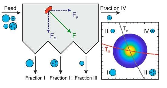
As example, a separation according to sedimentation with an orthogonal acting electrical field is chosen. The related parameters are the sedimentation coefficient s and electrical mobility µ. The separation functions will be denoted for the sedimentation and for the mobility. The forces which separate the feed particles are denoted FS and Fµ (see Figure 6). For the separations regarding sedimentation and mobility, the following values of the mean cut sizes are defined: scut ∈ with T1(scut) = 0.5 and µcut ∈ with T2 (µcut) = 0.5. Since there are two separations, the feed is subdivided into four basins, which are defined as:
I: s ≥ scut ∧ µ ≥ µcut coarse fraction with respect to both s and µ
II: s ≥ scut ∧ µ < µcut intermediate fraction (coarse for s, fine for µ)
III: s < scut ∧ µ ≥ µcut intermediate fraction (fine for s, coarse for µ)
IV: s < scut ∧ µ < µcut fine fraction with respect to both s and µ.
Each separation can be regarded as separation in one coarse (I), one fine (IV) and two intermediate fractions (II and III) with respect to the acting physical forces (Figure 7).
The two separation events can be regarded as independent because the acting forces are orthogonal to each other and no interaction between them is assumed, leading to the multiplication of the individual probabilities to obtain the probability for the combined event. The probability for a particle to be in basin , where the coarse material regarding both attributes is collected, is given by T1(s) T2(µ). Here it becomes evident that all investigations have to be performed based on the same set of parameters, namely the length and diameter; therefore, all quantities need to be expressed in terms of these parameters. The sedimentation coefficient is obtained via [22]
with the particle mass mparticle = V , volume of the particle , the particle density (gold bulk density) , the solvent density (water) , solvent viscosity η (water) and frictional ratio
where y is the logarithm of the aspect ratio y = [38] and the volume equivalent diameter of the particle . The electrical mobility is given in a simplified way [11] by
where the charge Q is the product of the particle surface area A multiplied with the surface density charge . The variables s and µ are linked to the geometric parameters (l, d) of the nanorod ensemble. Based on the integral mass balance, the feed PSD qFeed is given by the weighted sums of all basin PSDs and the related normalized mass fractions γi
The calculation of a missing PSD from a certain basin is possible, if all other PSDs including the feed and the relative amounts of the fractions are known
We summarize the product of the 1D separation efficiencies to T2D,I(l, d), which is the probability that a particle with (l, d), is in basin I (overall coarse fraction) and call it in the following the effective separation function for basin I. The PSD in fraction I can be determined—equivalent to Equation (6)—via
qFeed (l, d) is the number-weighted PSD, which is multiplied with the probability of a particle being in I and normalized a posteriori via
For the other basins, the PSDs can be determined similarly. The separation efficiency for basin IV (overall fines fraction), where the fines from both separations are collected, is (1−T1(s)) (1−T2(µ)). For the two intermediate basins, the particles belong to the coarse fraction of one attribute and to the fine fraction of the other one. Thus, we determine the efficiencies of fraction II with T1(s) (1−T2(µ)) and for fraction III with (1−T1(s)) T2(µ). The resulting separation functions for the four basins are illustrated in Figure 8a. The individual separation functions are not ideally sharp, resulting in qFeed(l, d) not beeing sharply divided into the four fractions. Therefore, the PSDs of the single fractions always contain particles from the other fractions as well; see Figure 8b. In summary, the PSDs resulting from two orthogonal separations are obtained via the following steps:
- Determine the individual separation functions as functions of the acting physical principles, e.g., T1(s), T2(µ);
- Translate the parameter-dependent functions to the set of the investigated parameters, e.g., length and diameter (l d)T;
- Determine the number of fractions;
- Determine if each fraction belongs to the coarse or fine fraction with respect to the individual separations;
- Calculate the effective separation functions for each basin;
- Calculate the PSD for each basin via the effective separation function and the prefactors γi.
The resulting distributions and separation efficiencies contain all relevant information for additional transformations, analogously to the previous sections. One important quantity is the amount of misplaced particles Λ, which can be obtained by conditional integration of the corresponding PSDs. For example, for fraction I the misplaced amount ΛI is in the regions where the sedimentation coefficient and mobility values are smaller than the previously defined cut sizes’ equivalent mean T-values; this corresponds to the fractions labelled II, III and IV.
4.3. Consecutive Separations
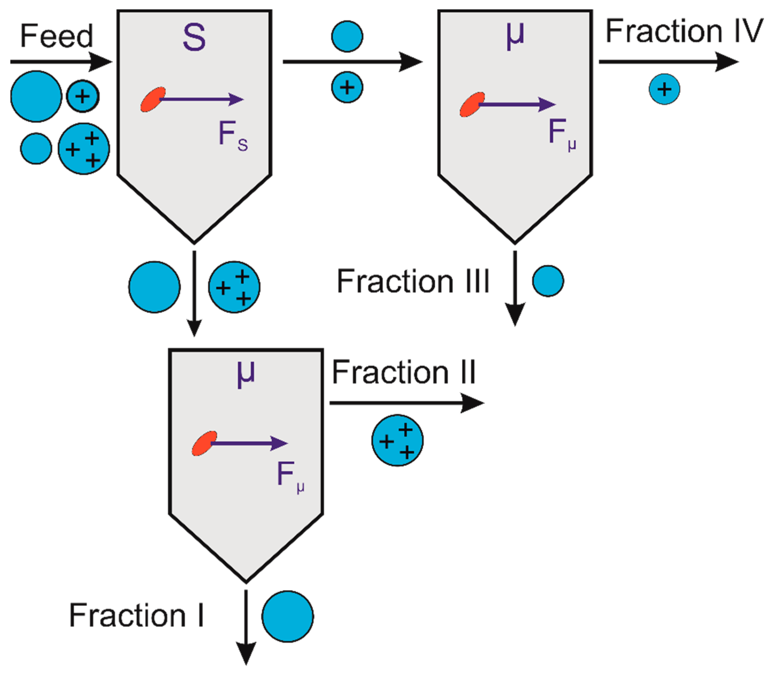
The separation with two acting orthogonal forces is similar to consecutive separations as shown in Figure 9. A prerequisite for the equivalence of simultaneous and consecutive separations is the ability to describe the separation process in terms of a perpendicular set of forces under the assumption of negligible interparticulate forces.
With the two separating forces acting perpendicularly, the particle motions can be considered independent of each other. In the first stage, the particles are separated in two fractions exhibiting either slow or fast sedimentation (s). Each fraction can then be separated individually according to its electric properties (µ), delivering similar fractions I-IV, as for the simultaneous separation apparatus. The consecutive separation from s to µ is applied to the coarse and to the fine fractions and results in four basins with four classes of particles: fast sedimenting neutral (I), fast sedimenting charged (II), slowly sedimenting neutral (III) and slowly sedimenting charged (IV) particles, as indicated in Figure 9. The separation function can be determined according to Equation (24) from particle trajectory calculations and the resulting final position of a particle with respect to the four basins.
For orthogonal separations, it does not matter if the two separations are performed simultaneously in one apparatus or in series in different apparatus. The more general case of non-orthogonal forces does not allow us to decouple the separation into individual separation steps independently of each other. In this case, the transport of the particle through the apparatus must be determined by full-scale particle-trajectory calculations, based on the flow and force fields in the apparatus. Today, coupled CFD-DEM simulations are widely used, which would also allow us to take also particle–particle interactions into account.
5. Generalization to M-Fold Orthogonal Separations Acting on Multidimensional PSDs
The investigation of multidimensional PSDs, which are subject to multi-fold separation processes, is a straightforward, generalized extension of the methodology outlined in Section 3. An nD number weighted PSD is separated in a distinct number of basins by separation processes. The number of basins is defined as and depends on the separation techniques used. The m separation functions are again expressed in the same coordinates that are used to describe the particle ensemble—the coordinates—and are denoted as with . The probability for a particle to be in certain basin is given by the multiplication of the m single probabilities resulting from the separation processes. Once again, each separation leads to a separation of the feed into coarse and fine fractions. For these, we can define two sets of separation processes for each basin
which contain all separations that sort into basin j. With these sets, the calculation of the PSD in the basin j can be expressed as
with the effective separation function for the basin , which is calculated via the multiplications from the two product functions, . Similar to the 2D case, the prefactor γj still yields the same information—the amount of particles in the basin j—and can be obtained via a posteriori normalization of the separation result from the global mass balance
We note here that with γj and given, the original PSD can be reconstructed as
This equation holds, since each particle has to belong to exactly one fraction and therefore the probabilities sum up to 1. With this in mind, we can also reconstruct a PSD , with r ∈ {1,…, m }, if the other PSDs and are known. In this case we determine
6. Examples of Technical Realizations
6.1. Hydrocyclone: Fractionation with Respect to Size and Shape
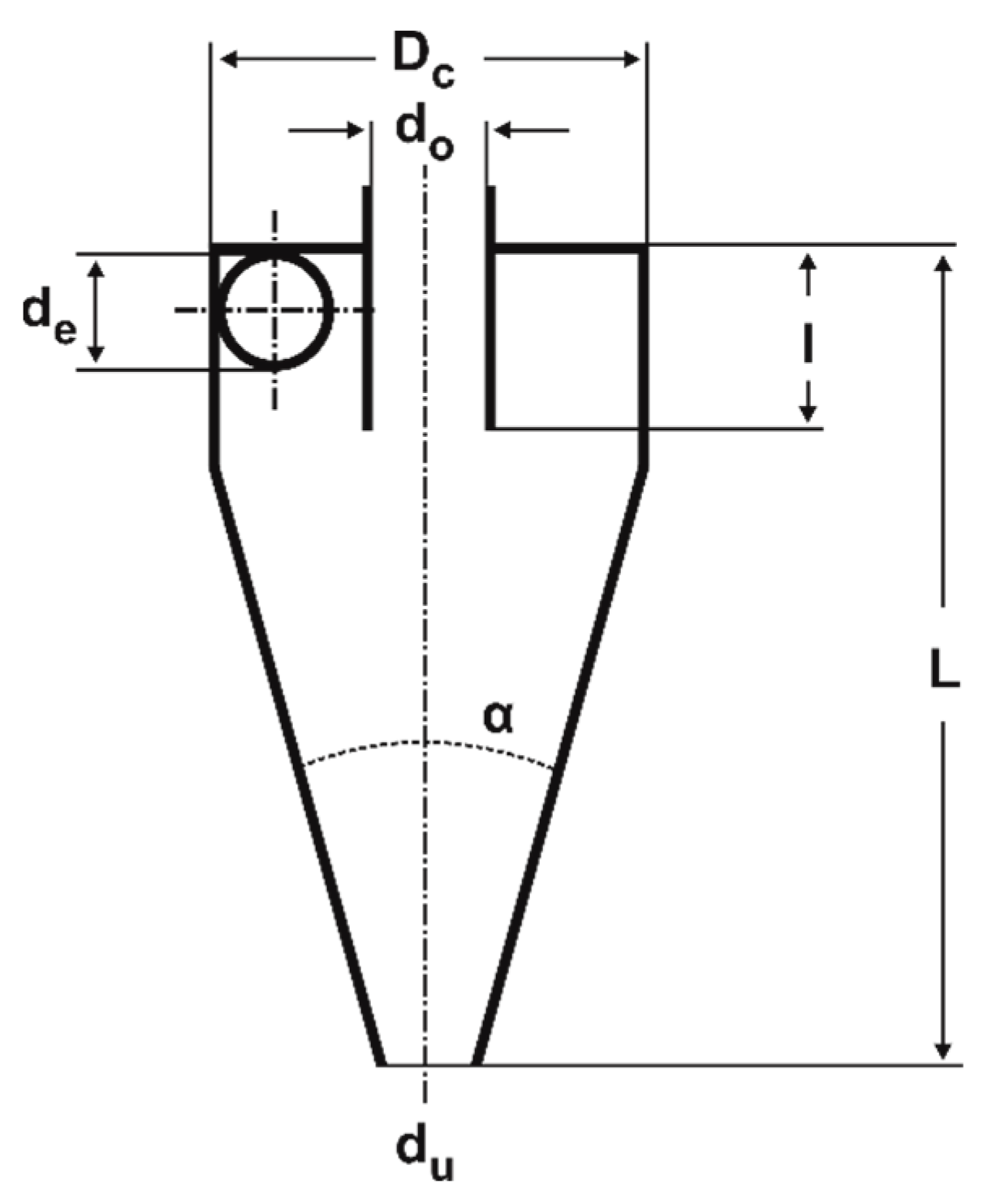
Hydrocyclones are used to separate solid or liquid particles from a liquid phase by centrifugal forces. The advantage of the hydrocyclone over other centrifugal separators is that no moving parts are used (Figure 10). Hydrocyclones are widely applied in the mineral, starch and offshore industries.
This example is related to a recently developed process in our group to deform spherical glass particles to platelets below the brittle–ductile transition in a stirred media mill [37,39]. We assume a quadratic volume based PSD (q3) of spheres between 2–7 µm. These spheres are deformed into cylinders with a final thickness of l = 200 nm using a stirred-media ball mill. During compression, the particle density increases due to internal densification; for calculations, it is assumed that the density increases linearly from 100% (spheres) to 110% for fully deformed particles with a final thickness of 200 nm. The resulting number-weighted PSDs of the spheres (starting shape) and the plates with a thickness of 200 nm (final shape) are shown in a 2D diagram in Supporting Information, Figure S1. In order to obtain a realistic distribution of the particle ensemble during this process, the different stages between spheres and cylinders with a final thickness of 200 nm are calculated via the aspect ratio (l/d). At each stage, the aspect ratio (l/d) is assumed to be normally distributed. The resulting PSD of the feed can be seen in Figure 11b.
For the separation of the feed, a hydrocyclone with a geometry according to Rietema (Supporting information, Table S1) is designed. The cut size xcut can be calculated using the Reynolds number Re (33), the Euler number Eu (32) and the product of the Stokes and Euler number Stk50Eu (31), as described in the literature [40]. The values of the constants ki and ni (Supplementary Materials Table S2) are dependent on the geometry of the cyclone and can be taken from the literature for Rietema cyclones [41]:
By assuming a feed flow rate of 15 L/min, a feed concentration cV of 5%, a liquid density of pentanol of = 810 kg/m³, a solid density of silica particles of = 2200 kg/m³ and liquid viscosity of 3.68 mPas as operation parameters, a cut size xcut of 4.8 μm results. The corresponding hydrocyclone diameter is 10 cm, the pressure drop is 39.7 bar and the water flow ratio RW is 7.4%. Similar hydrocyclone sizes and pressure drops can also be found in the literature [42]. Using the classical equation of Rosin and Rammler as proposed by Plitt, the corrected separation function can be calculated using (35). For the purpose of simplicity and comprehensibility of the example, the corrected separation function is used:
T(x)′ is corrected to avoid the typical fish hook and spans from 0 to 1. Here, the parameter b is a measure for the sharpness of separation. For Rietema hydrocyclones, a value of 2.45 is used, which corresponds to a separation sharpness of 53%. dC refers to a characteristic diameter of the particle. In the case of a sphere, dC is the sphere diameter, but in the case of deviating geometries, form factors must be applied.
Particle shape influences separation through the shape-dependent movement of the particles through the hydrocyclone. The separation efficiency can be modelled by taking into account all forces acting on the particles (in particular centrifugal, gravitational and drag forces) [43].
For simplicity, we only refer to the fundamental balance of centrifugal and drag forces and neglect the complicated motion of non-spherical particles. Here, the centrifugal force acts on the volume of the particle ( and the drag force acts on the cross-section ( of the particle. By assuming a steady state and laminar flow conditions in the Stokes regime, the equation of motion simplifies to (39), where the form factor enters with an exponent of −0.25. Thereby, the chosen form factor (38) is defined as the ratio of the diameter of the volume equal sphere xV to the diameter of the projection area equal sphere xA and ranges between 1 (sphere) and 0. This is similar to the well-known sphericity according to Wadell, but relates the volume equivalent diameter to the diameter of the same projection area rather than the same surface area. Thus, as integrated into the separation function as can be seen in (40):
In the case of the cylinders, it can be assumed that they are oriented in such a way that they show their minimum projection area in the main flow direction (circular path in the hydrocyclone) in order to minimize the drag force. Therefore, for the radial movement of the cylinders, the maximum projection area is included in the drag force (xA = d) [43].
The results depicted in Figure 11 show the corrected separation function and the PSD of the feed, as well as the coarse fraction and the fine fraction, in 2D space.
Figure 11a shows the 2D separation function. It can be clearly seen from the isolines of the same volume that the separation performance improves with increasing deformation from sphere to plate. The reason for this is the increasing cross-section of the particles with increasing deformation, which raises the drag force. This enables the separation of spheres and plates. As can be seen in Figure 11b, the feed consists of spheres (d/l ratio = 1) and plate-shaped cylinders (d/l ratio > 1) up to a minimum thickness of 200 nm. Applying the separation function (Figure 11a) to the feed distribution results in the fine fraction and coarse fraction. The separation is most clearly visible in the coarse material. Here, the peak of the distribution shifts from a diameter of 4.4 µm and a length of 0.7 µm towards larger diameters of 10.2 µm and shorter length of 0.3 µm, i.e., more plate-shaped particles. The fines with the more spherical particles can be sent back to the mill for further deformation. This enables a quasi-continuous operation of the process, in which the coarse material is separated after fixed time intervals and the fine material is fed back into the mill with new feed material.
6.2. Disc Separator: Fractionation with Respect to Size and Density Separation
Finally, we extend the classification to a size- and density-distributed particle ensemble using a disc separator (disc stack centrifuge), where the separation depends on the particle size as well as the density difference between the liquid and solid phase function (Figure 12).
Details on the design and operating principle can be found in the literature [45,46]. The separation function of a disc separator can be estimated from [47]
where ρp and ρf are the particle and fluid density, x the diameter of the particles, ra and ri the outer and inner radius of the discs, f the fluid viscosity and α the angle of the discs; see Supporting Information, Table S3, for the values of the material properties. The angular velocity ω is calculated from the rotational speed n by
Assuming that the feed is equally distributed among the individual disc gaps, the flow rate of each disc gap T is expressed by
where is the total feed volume flow and N the number of disc gaps. In the Supporting Information, Table S3, the material parameters and the dimensions of the centrifuge are listed.
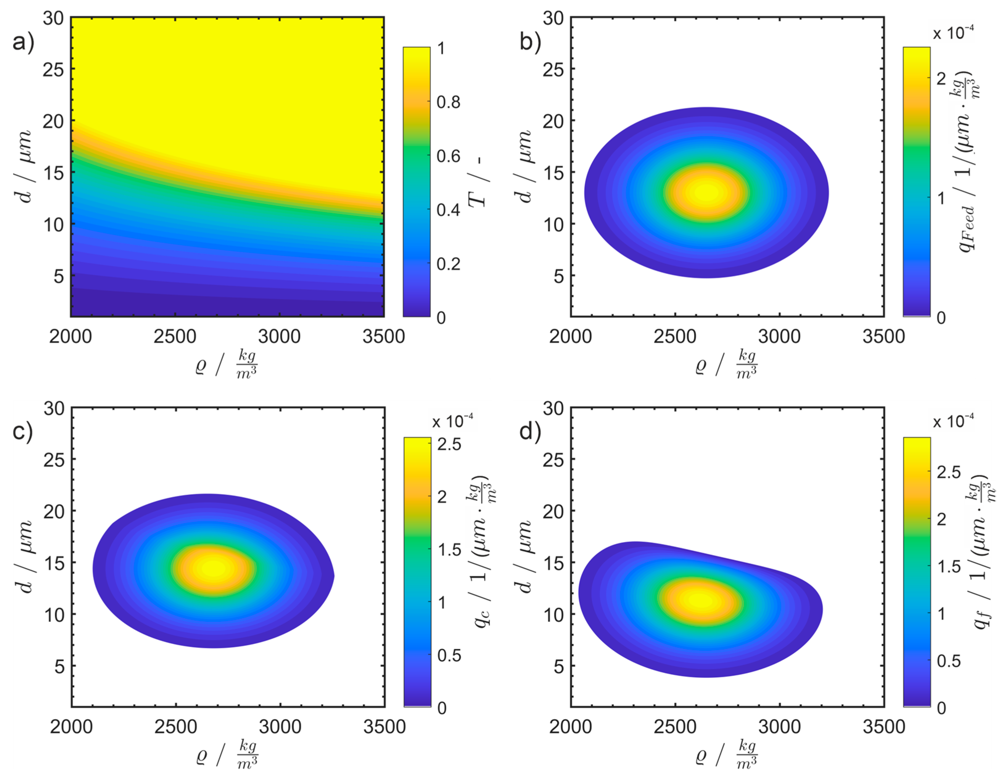
For the calculations, a size- and density-distributed particle system as shown in Figure 13a is assumed. Using Equation (43) and the material and geometric data in the SI, the separation function T(d, ρp) is then calculated (see Figure 13b). The corresponding PSDs of the coarse and fine fraction are given in Figure 13c,d.
As can be seen from the initial distribution in Figure 13a, the feed consists of particles with a mean size of ~13 µm and a mean density of ~2650 . After classification with the disc separator by applying Equation (43) to the feed distribution, the initial particle size and density distribution is classified into a coarse and fine fraction. While the distribution of the feed dispersion lies within the range ~5 µm to ~21 µm and ~2050 kgm−3 to 3250 kgm−3, the distribution of the coarse fraction ranges from ~7 µm to ~21 µm and ~2100 kgm−3 to ~3250 kgm−3. Therefore, all particles below 7 µm and particles with a density smaller than 2100 kgm−3 are completely classified into the fine fraction. Particles larger than 17 µm and particles with a density higher than 3200 kgm−3 can be found only the coarse fraction. Thus, the center of the coarse fraction is shifted to ~14 µm and ~2700 kgm−3 and the center of the fine fraction is observed at ~11 µm and ~2600 kgm−3.
7. Conclusions
Based on the comprehensive mathematical framework for multidimensional particle size and property distributions [1] and the ways of calculating these illustrated [20,21,48], we describe one or higher dimensional separation processes for the fractionation of nD property distributions. As a particular example, we discuss the separation processes of 2D PSDs for nanorods, where we distinguish between a single separation step, two orthogonal separations and consecutive and simultaneous separation, as well as non-orthogonal and interacting separations.
A simultaneous separation according to two physical quantities can be described as two consecutive separations in the case of two perpendicular acting separation forces. For the two orthogonal separations, a fractionation according to sedimentation and electrical mobility is chosen as example. This leads to the classification of the feed into four fractions. The non-orthogonal superposition of two field forces is the most complex case and requires full particle-trajectory calculations.
The mathematical framework is generalized to m-fold orthogonal separations on multidimensional PSDs. The number of fractions depends upon the number and kind of applied separation processes, where each separation process can be considered individually with its individual coarse and fine fraction. This leads to a superposition of all separation functions and effective separation functions for each fraction. As illustrative simplified examples, we present shape-selective separations in hydrocyclone and density-dependent separations in a disc centrifuge. Building on the presented framework, studies on the chromatographic separations of nanoparticles are underway.
Supplementary Materials
The following supporting information can be downloaded at: https://www.mdpi.com/article/10.3390/separations10040252/s1, Figure S1: Number-weighted particle size distribution q0 of the sphere (l = d) and the spheres deformed into cylinders with a thickness of 0.2 µm shown in a 3D diagram; Table S1: Geometry of Rietema hydrocyclones; Table S2: Constants k and n for different hydrocyclone designs; Table S3: Material properties and geometrical data of the disc separator. References [41,49] are cited in the Supplementary Materials.
Author Contributions
U.F.: Conceptualization, data curation, formal analysis, investigation; methodology, project administration, visualization, writing—original draft, writing—review and editing. J.D.: Data curation, formal analysis, investigation, methodology, writing—review and editing. F.T.: Formal analysis, investigation, visualization, Writing—original draft; writing—review and editing. S.E.W.: Conceptualization, writing—original draft. L.G.: Formal analysis, Investigation; Visualization; Writing—original draft; writing—review and editing. J.W.: Writing—review and editing. F.L.: Formal analysis, Writing—review and editing. W.P.: Conceptualization, resources, Writing—original draft; Writing—review and editing, supervision, funding acquisition. All authors have read and agreed to the published version of the manuscript.
Funding
This research was funded by the Deutsche Forschungsgemeinschaft (DFG, German Research Foundation) within SPP 2045 “Highly specific and multidimensional fractionation of fine particle systems with technical relevance” (Project-ID 313858373), CRC 814 “Additive Manufacturing” (Project-ID 61375930) and SFB 1411 Design of Particulate Product (Project-ID 416229255).
Data Availability Statement
The data that support the findings of this study are available from the corresponding author, upon reasonable request.
Acknowledgments
We gratefully acknowledge financial support by Deutsche Forschungsgemeinschaft and Friedrich-Alexander-Universität Erlangen-Nürnberg within the funding program “Open Access Publication Funding.
Conflicts of Interest
The authors declare no conflict of interest.
Abbreviations
| µ | electrical mobility |
| aZ | centrifugal acceleration |
| B | number of basins |
| b | measure for the sharpness of separation |
| c | coarse fraction |
| cV | volume concentration |
| d | diameter of a cylinder |
| DC | hydrocyclone diameter |
| Eu | Euler number |
| f | fine fraction |
| f/f0 | frictional ratio |
| FD | drag force |
| FZ | centrifugal force |
| l | length |
| M | mass |
| Mc,r | r weighted amounts of particle |
| Mr,k | moment |
| N | number of disc gaps |
| nD | n-dimensional |
| PSD | particle size distribution |
| qr(x) | r weighted property density distribution |
| Qr(x) | r weighted property sum distribution |
| qr(x) | charge |
| RW | water flow ratio |
| Re | Reynolds number |
| s | sedimentation coefficient |
| T(x) | separation efficiency |
| T(x)′ | corrected separation efficiency |
| V | volume |
| flow rate | |
| x | particle diameter |
| xcut | cut size |
| α | angle |
| γi | normalized mass fractions |
| ΔP | pressure drop |
| η | solvent density |
| κ(x) | a weighting function |
| Λi | yield |
| density | |
| ϕ | form factor |
| ω | angular velocity |
References
- Frank, U.; Wawra, S.E.; Pflug, L.; Peukert, W. Multidimensional Particle Size Distributions and Their Application to Nonspherical Particle Systems in Two Dimensions. Part. Part. Syst. Charact. 2019, 36, 1800554. [Google Scholar] [CrossRef]
- Backes, C.; Higgins, T.M.; Kelly, A.; Boland, C.; Harvey, A.; Hanlon, D.; Coleman, J.N. Guidelines for Exfoliation, Characterization and Processing of Layered Materials Produced by Liquid Exfoliation. Chem. Mater. 2017, 29, 243–255. [Google Scholar] [CrossRef]
- Knieke, C.; Berger, A.; Voigt, M.; Taylor, R.N.K.; Röhrl, J.; Peukert, W. Scalable production of graphene sheets by mechanical delamination. Carbon 2010, 48, 3196–3204. [Google Scholar] [CrossRef]
- Völkl, A.; Klupp Taylor, R.N. Investigation and mitigation of reagent ageing during the continuous flow synthesis of patchy particles. Chem. Eng. Res. Des. 2022, 181, 133–143. [Google Scholar] [CrossRef]
- Akdas, T.; Walter, J.; Segets, D.; Distaso, M.; Winter, B.; Birajdar, B.; Spiecker, E.; Peukert, W. Investigation of the size-property relationship in CuInS2 quantum dots. Nanoscale 2015, 7, 18105–18118. [Google Scholar] [CrossRef] [Green Version]
- Ahmad, R.; Brandl, M.; Distaso, M.; Herre, P.; Spiecker, E.; Hock, R.; Peukert, W. A comprehensive study on the mechanism behind formation and depletion of Cu2 ZnSnS4 (CZTS) phases. CrystEngComm 2015, 17, 6972–6984. [Google Scholar] [CrossRef] [Green Version]
- Nitta, N.; Wu, F.; Lee, J.T.; Yushin, G. Li-ion battery materials: Present and future. Mater. Today 2015, 18, 252–264. [Google Scholar] [CrossRef]
- Winkler, M.; Rhein, F.; Nirschl, H.; Gleiss, M. Real-Time Modeling of Volume and Form Dependent Nanoparticle Fractionation in Tubular Centrifuges. Nanomaterials 2022, 12, 3161. [Google Scholar] [CrossRef]
- Plüisch, C.S.; Bössenecker, B.; Dobler, L.; Wittemann, A. Zonal rotor centrifugation revisited: New horizons in sorting nanoparticles. RSC Adv. 2019, 9, 27549–27559. [Google Scholar] [CrossRef] [Green Version]
- Leschonski, K. The feasibility of producing small cut sizes in an electrostatic classifier. Powder Technol. 1987, 51, 49–59. [Google Scholar] [CrossRef]
- Thajudeen, T.; Walter, J.; Srikantharajah, R.; Lübbert, C.; Peukert, W. Determination of the length and diameter of nanorods by a combination of analytical ultracentrifugation and scanning mobility particle sizer. Nanoscale Horiz. 2017, 2, 253–260. [Google Scholar] [CrossRef] [PubMed]
- Barasinski, M.; Hilbig, J.; Neumann, S.; Rafaja, D.; Garnweitner, G. Simple model of the electrophoretic migration of spherical and rod-shaped Au nanoparticles in gels with varied mesh sizes. Colloids Surf. A Physicochem. Eng. Asp. 2022, 651, 129716. [Google Scholar] [CrossRef]
- Segets, D.; Komada, S.; Butz, B.; Spiecker, E.; Mori, Y.; Peukert, W. Quantitative evaluation of size selective precipitation of Mn-doped ZnS quantum dots by size distributions calculated from UV/Vis absorbance spectra. J. Nanopart. Res. 2013, 15, 1486. [Google Scholar] [CrossRef]
- Michaud, V.; Pracht, J.; Schilfarth, F.; Damm, C.; Platzer, B.; Haines, P.; Harreiß, C.; Guldi, D.M.; Spiecker, E.; Peukert, W. Well-separated water-soluble carbon dots via gradient chromatography. Nanoscale 2021, 13, 13116–13128. [Google Scholar] [CrossRef]
- Hersam, M.C. Progress towards monodisperse single-walled carbon nanotubes. Nat. Nanotechnol. 2008, 3, 387–394. [Google Scholar] [CrossRef]
- Gromotka, L.; Uttinger, M.J.; Schlumberger, C.; Thommes, M.; Peukert, W. Classification and characterization of multimodal nanoparticle size distributions by size-exclusion chromatography. Nanoscale 2022, 14, 17354–17364. [Google Scholar] [CrossRef]
- Süβ, S.; Bartsch, K.; Wasmus, C.; Damm, C.; Segets, D.; Peukert, W. Chromatographic property classification of narrowly distributed ZnS quantum dots. Nanoscale 2020, 12, 12114–12125. [Google Scholar] [CrossRef]
- Backes, C.; Szydłowska, B.M.; Harvey, A.; Yuan, S.; Vega-Mayoral, V.; Davies, B.R.; Zhao, P.-L.; Hanlon, D.; Santos, E.J.G.; Katsnelson, M.I.; et al. Production of Highly Monolayer Enriched Dispersions of Liquid-Exfoliated Nanosheets by Liquid Cascade Centrifugation. ACS Nano 2016, 10, 1589–1601. [Google Scholar] [CrossRef]
- Buchwald, T.; Ditscherlein, R.; Peuker, U.A. Beschreibung von Trennoperationen mit mehrdimensionalen Partikeleigenschaftsverteilungen. Chem. Ing. Tech. 2023, 95, 199–209. [Google Scholar] [CrossRef]
- Frank, U.; Uttinger, M.J.; Wawra, S.E.; Lübbert, C.; Peukert, W. Progress in Multidimensional Particle Characterization. KONA Powder Part. J. 2022, 39, 3–28. [Google Scholar] [CrossRef]
- Wawra, S.E.; Pflug, L.; Thajudeen, T.; Kryschi, C.; Stingl, M.; Peukert, W. Determination of the two-dimensional distributions of gold nanorods by multiwavelength analytical ultracentrifugation. Nat. Commun. 2018, 9, 4898. [Google Scholar] [CrossRef] [PubMed]
- Walter, J.; Gorbet, G.; Akdas, T.; Segets, D.; Demeler, B.; Peukert, W. 2D analysis of polydisperse core-shell nanoparticles using analytical ultracentrifugation. Analyst 2016, 142, 206–217. [Google Scholar] [CrossRef] [PubMed] [Green Version]
- Frank, U.; Drobek, D.; Sanchez-Iglesias, A.; Wawra, S.; Nees, N.; Walter, J.; Pflug, L.; Apeleo Zubiri, B.; Spiecker, E.; Liz-Marzan, L.; et al. Determination of 2D particle size distributions in plasmonic nanoparticle colloids via analytical ultracentrifugation - Application to gold bipyramids. ACS Nano 2023, 17, 5785–5798. [Google Scholar] [CrossRef] [PubMed]
- Furat, O.; Leißner, T.; Ditscherlein, R.; Šedivý, O.; Weber, M.; Bachmann, K.; Gutzmer, J.; Peuker, U.; Schmidt, V. Description of Ore Particles from X-Ray Microtomography (XMT) Images, Supported by Scanning Electron Microscope (SEM)-Based Image Analysis. Microsc. Microanal. 2018, 24, 461–470. [Google Scholar] [CrossRef]
- Buchmann, M.; Schach, E.; Tolosana-Delgado, R.; Leißner, T.; Astoveza, J.; Kern, M.; Möckel, R.; Ebert, D.; Rudolph, M.; van den Boogaart, K.; et al. Evaluation of Magnetic Separation Efficiency on a Cassiterite-Bearing Skarn Ore by Means of Integrative SEM-Based Image and XRF–XRD Data Analysis. Minerals 2018, 8, 390. [Google Scholar] [CrossRef] [Green Version]
- Segets, D.; Lutz, C.; Yamamoto, K.; Komada, S.; Süß, S.; Mori, Y.; Peukert, W. Classification of Zinc Sulfide Quantum Dots by Size: Insights into the Particle Surface–Solvent Interaction of Colloids. J. Phys. Chem. C 2015, 119, 4009–4022. [Google Scholar] [CrossRef]
- Leschonski, K.; Alex, W.; Koglin, B. Teilchengrößenanalyse. 1. Darstellung und Auswertung von Teilchengrößenverteilungen. Chem. Ing. Tech. 1974, 46, 23–26. [Google Scholar] [CrossRef]
- Leschonski, K.; Alex, W.; Koglin, B. Teilchengrößenanalyse. 1. Darstellung und Auswertung von Teilchengrößenverteilungen (Fortsetzung). Chem. Ing. Tech. 1974, 46, 101–106. [Google Scholar] [CrossRef]
- Stiess, M. Mechanische Verfahrenstechnik—Partikeltechnologie 1, 3rd ed.; Springer: Berlin/Heidelberg, Germany, 2009; ISBN 978-3-540-32551-2. [Google Scholar]
- Modena, M.M.; Rühle, B.; Burg, T.P.; Wuttke, S. Nanoparticle Characterization: What to Measure? Adv. Mater. 2019, 31, e1901556. [Google Scholar] [CrossRef]
- Coulson, J.M.; Richardson, J.F. Coulson and Richardson’s Chemical Engineering, 6th ed.; Butterworth-Heinemann: Amsterdam, The Netherlands, 2018; ISBN 9780081010976. [Google Scholar]
- Liang, S. Numerical Study of Classification of Ultrafine Particles in a Gas-Solid Field of Elbow-Jet Classifier. Chem. Eng. Commun. 2010, 197, 1016–1032. [Google Scholar] [CrossRef]
- Giddings, J.C. Field-flow fractionation: Analysis of macromolecular, colloidal, and particulate materials. Science 1993, 260, 1456–1465. [Google Scholar] [CrossRef] [PubMed]
- Schach, E.; Buchmann, M.; Tolosana-Delgado, R.; Leißner, T.; Kern, M.; van den Gerald Boogaart, K.; Rudolph, M.; Peuker, U.A. Multidimensional characterization of separation processes—Part 1: Introducing kernel methods and entropy in the context of mineral processing using SEM-based image analysis. Miner. Eng. 2019, 137, 78–86. [Google Scholar] [CrossRef]
- Buchmann, M.; Schach, E.; Leißner, T.; Kern, M.; Mütze, T.; Rudolph, M.; Peuker, U.A.; Tolosana-Delgado, R. Multidimensional characterization of separation processes—Part 2: Comparability of separation efficiency. Miner. Eng. 2020, 150, 106284. [Google Scholar] [CrossRef]
- Cardenas Lopez, P.; Uttinger, M.J.; Traoré, N.E.; Khan, H.A.; Drobek, D.; Apeleo Zubiri, B.; Spiecker, E.; Pflug, L.; Peukert, W.; Walter, J. Multidimensional characterization of noble metal alloy nanoparticles by multiwavelength analytical ultracentrifugation. Nanoscale 2022, 14, 12928–12939. [Google Scholar] [CrossRef] [PubMed]
- Esper, J.D.; Liu, L.; Willnauer, J.; Strobel, A.; Schwenger, J.; Romeis, S.; Peukert, W. Scalable production of glass flakes via compression in the liquid phase. Adv. Powder Technol. 2020, 31, 4145–4156. [Google Scholar] [CrossRef]
- Hansen, S. Translational friction coefficients for cylinders of arbitrary axial ratios estimated by Monte Carlo simulation. J. Chem. Phys. 2004, 121, 9111–9115. [Google Scholar] [CrossRef] [PubMed]
- Esper, J.D.; Maußner, F.; Romeis, S.; Zhuo, Y.; Barr, M.K.S.; Yokosawa, T.; Spiecker, E.; Bachmann, J.; Peukert, W. SiO2–GeO2 Glass–Ceramic Flakes as an Anode Material for High-Performance Lithium-Ion Batteries. Energy Tech. 2022, 10, 2200072. [Google Scholar] [CrossRef]
- Coelho, M.; Medronho, R. A model for performance prediction of hydrocyclones. Chem. Eng. J. 2001, 84, 7–14. [Google Scholar] [CrossRef]
- Castilho, L.R.; Medronho, R.A. A simple procedure for design and performance prediction of Bradley and Rietema hydrocyclones. Miner. Eng. 2000, 13, 183–191. [Google Scholar] [CrossRef]
- Neesse, T.; Dueck, J.; Schwemmer, H.; Farghaly, M. Using a high pressure hydrocyclone for solids classification in the submicron range. Miner. Eng. 2015, 71, 85–88. [Google Scholar] [CrossRef]
- Niazi, S.; Habibian, M.; Rahimi, M. A Comparative Study on the Separation of Different-Shape Particles Using a Mini-Hydrocyclone. Chem. Eng. Technol. 2017, 40, 699–708. [Google Scholar] [CrossRef]
- Tarleton, E.S.; Wakeman, R.J. Solid/Liquid Separation Equipment. Solid/Liquid Separation; Elsevier: Amsterdam, The Netherlands, 2007; pp. 1–77. ISBN 9781856174213. [Google Scholar]
- Mannweiler, K.; Hoare, M. The scale-down of an industrial disc stack centrifuge. Bioprocess Eng. 1992, 8, 19–25. [Google Scholar] [CrossRef]
- Maybury, J.P.; Mannweiler, K.; Titchener-Hooker, N.J.; Hoare, M.; Dunnill, P. The performance of a scaled down industrial disc stack centrifuge with a reduced feed material requirement. Bioprocess Eng. 1998, 18, 191. [Google Scholar] [CrossRef]
- Piesche, M.; Zink, A.; Schütz, S. Strömungs- und Trennverhalten von Tellerseparatoren zur Abscheidung von Ölnebelaerosolen, Untersuchungen zum Rotor/Rotor-Konzept. Chem. Ing. Tech. 2008, 80, 1487–1500. [Google Scholar] [CrossRef]
- Furat, O.; Frank, U.; Weber, M.; Wawra, S.; Peukert, W.; Schmidt, V. Estimation of bivariate probability distributions of nanoparticle characteristics, based on univariate measurements. Inverse Probl. Sci. Eng. 2021, 29, 1343–1368. [Google Scholar] [CrossRef]
- Rietema, K. Performance and design of hydrocyclones—III: Separating power of the hydrocyclone. Chem. Eng. Sci. 1961, 15, 310–319. [Google Scholar] [CrossRef]
Figure 1.
Differently weighted 2D length-diameter PSDs of gold nanorods. Depicted are the modal values (stars) for number (, blue), surface (, cyan) and volume (, yellow) weighted distributions with an isoline that corresponds to a value of max . Reproduced with permission from [1]. Copyright 2019, Wiley.
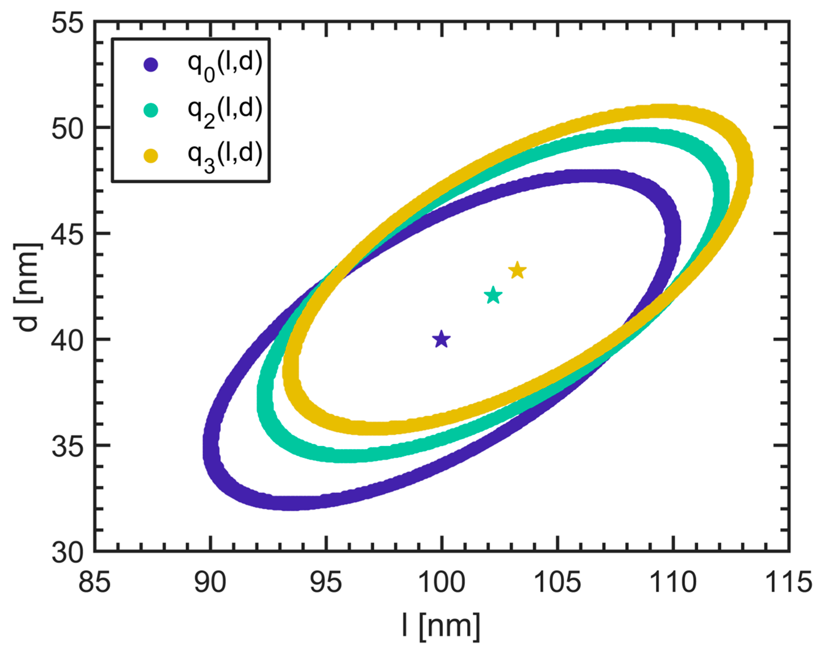
Figure 2.
Schematic drawing of a separation apparatus. A particle (red) is dragged by a force F (blue vector) to different locations within the apparatus. The particle is transported either to the coarse or fine fraction.
Figure 2.
Schematic drawing of a separation apparatus. A particle (red) is dragged by a force F (blue vector) to different locations within the apparatus. The particle is transported either to the coarse or fine fraction.
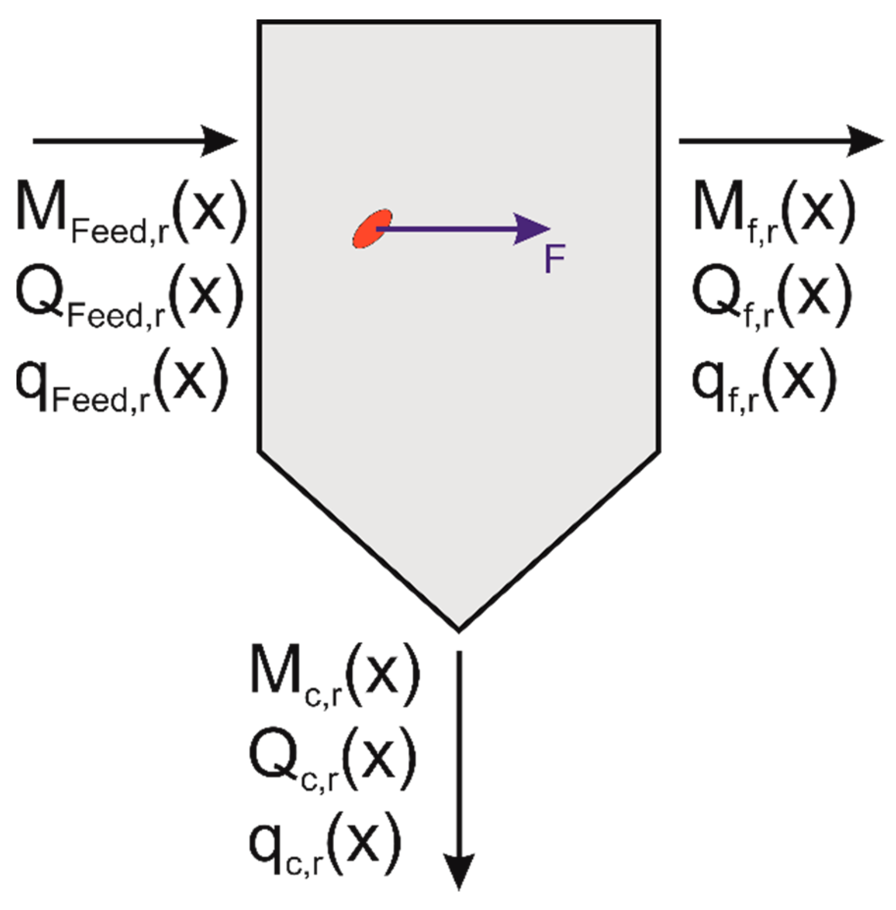
Figure 3.
(a) Example for a monomodal 1D number-based PSD (blue) with separation function (red). The grey lines indicate the 0.25, 0.5 and 0.75 values for the separation function in ascending order. The 0.25 and 0.75 values are commonly used for the calculation of the separation sharpness, while the 0.5 value is the cut size. (b) 1D PSD (blue) with resulting PSDs (dashed magenta) and (dashed green) after the separation process. The grey lines indicate the 0.25, 0.5 and 0.75 values for the separation function.
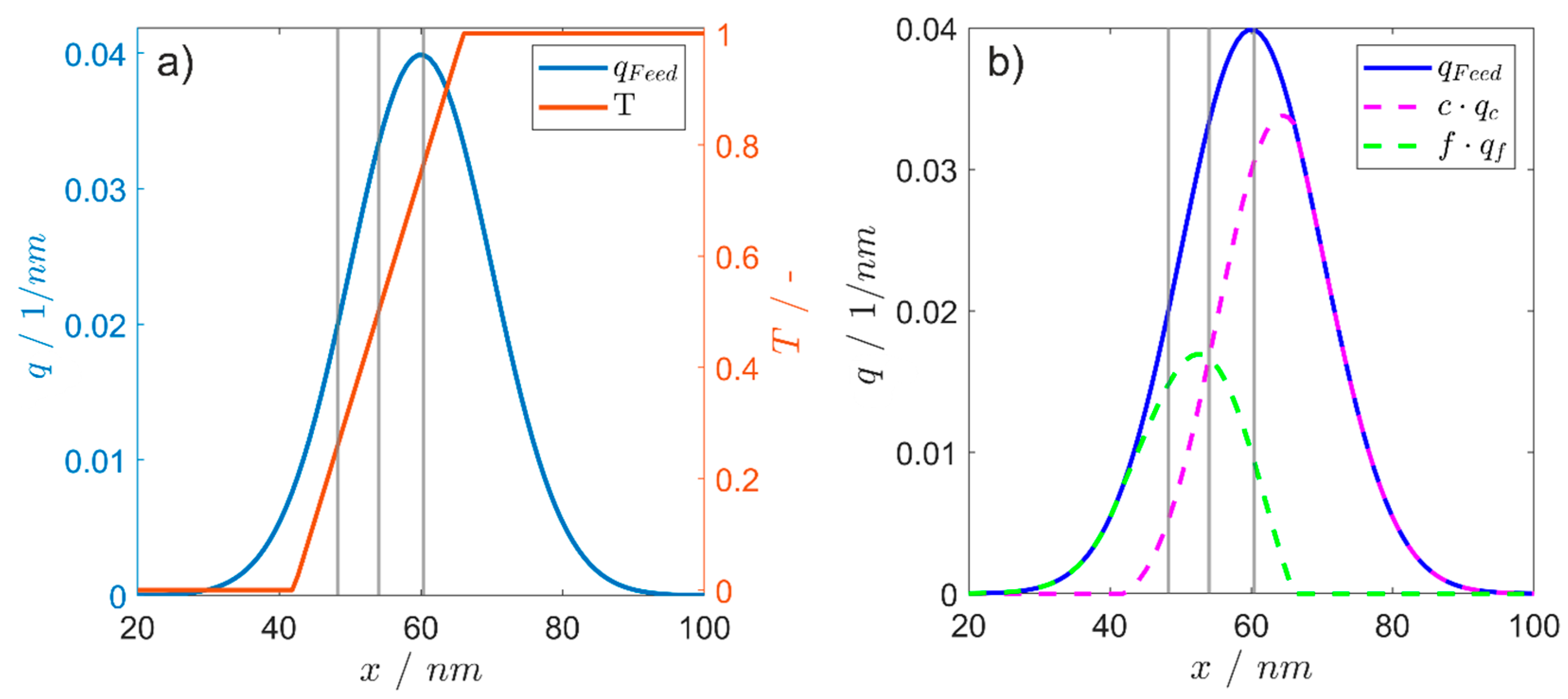
Figure 4.
(a) 1D volume-dependent separation function for the gold nanorods T(V). Between two volume values, the lower boundary (red line) and the upper limit of the volumes (green line) a linear function mimics the volume-dependent separation behavior; the black line marks the cut size with T(Vcut) = 0.5. (b) Translation of T(V) in the 2D length-diameter space as V(l, d). The illustrated isolines belong to the lower and upper boundaries and to the cut size from the left-handed plot. They are displayed in the same color. Small particles, in the sense of small length-diameter value combinations in the investigated 2D space, possess a smaller volume and have a lower probability to be sorted in the coarse fraction.

Figure 5.
(a) 2D Gaussian PSD of gold nanorods with isolines for the separation function values with T(Vcut) = 0.5 (black), T = 0, (red), T = 1 (green). The volume belonging to T(Vcut) = 0.5 corresponds to an isoline through the mean length-diameter value. The figure indicates that the PSD is split in a coarse and a fine fraction. The resulting PSDs of the coarse fraction are depicted in (b) and the PSD of the fine fraction in (c). Misplaced particles are visible as contributions below the black line for the coarse material and above the black line for the fine material.
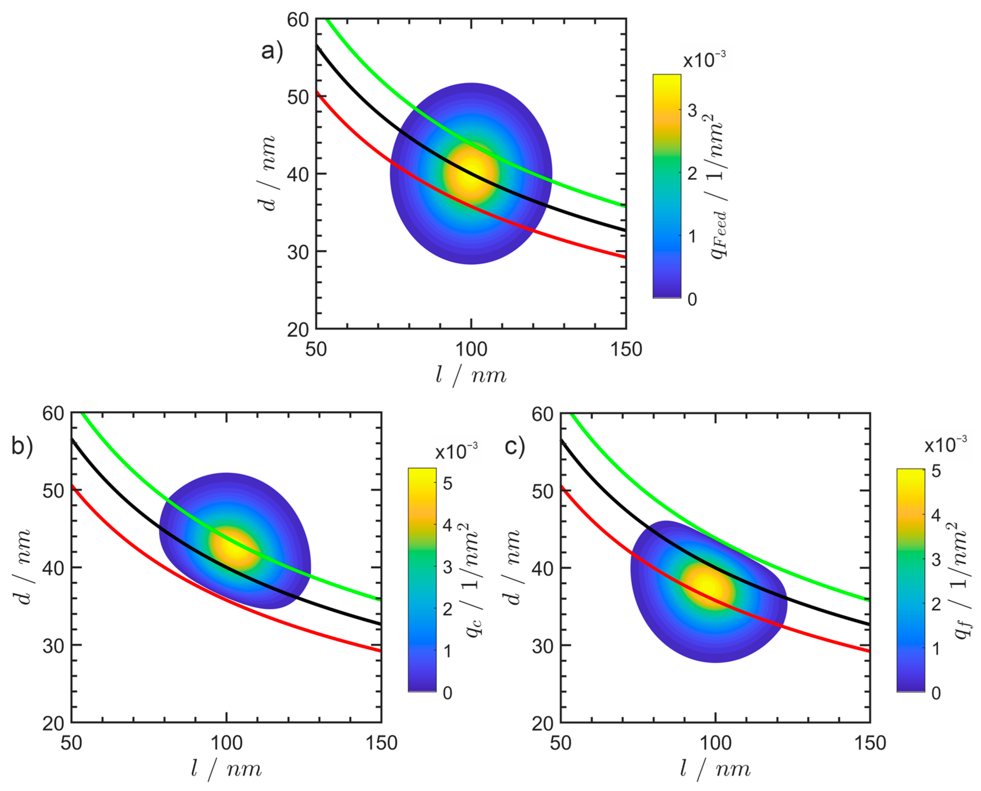
Figure 6.
Simultaneous separation with respect to two acting forces FS and Fµ, mass flows corresponding to consecutive separation.
Figure 6.
Simultaneous separation with respect to two acting forces FS and Fµ, mass flows corresponding to consecutive separation.
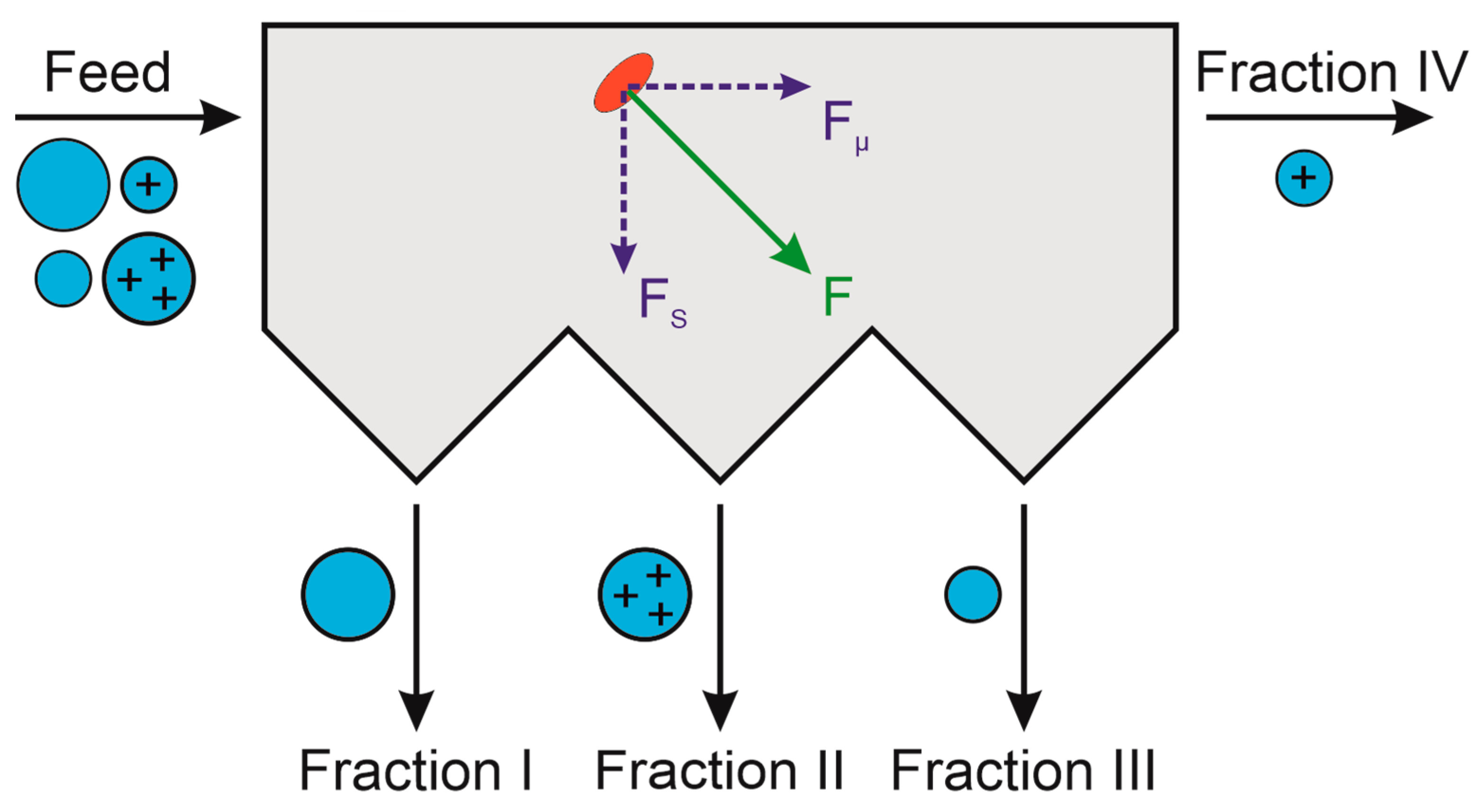
Figure 7.
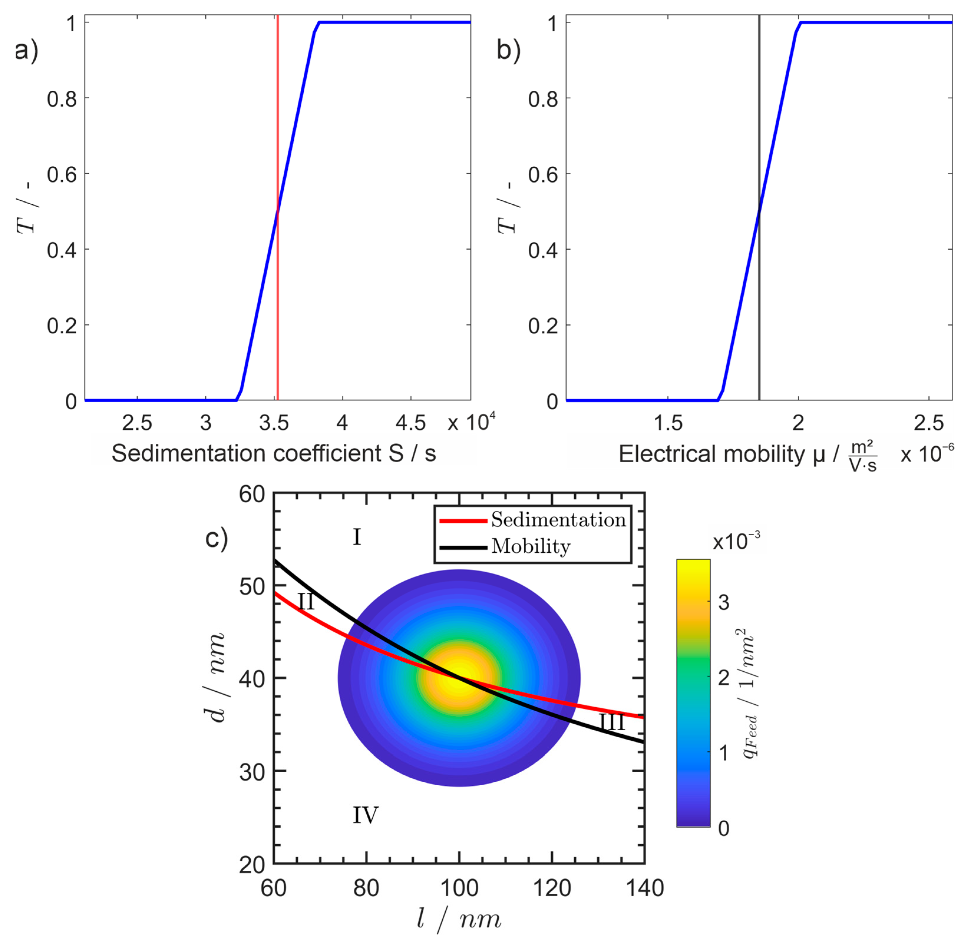
The assumed linear separation efficiencies for (a) a separation function with respect to sedimentation s and (b) a separation with respect to electrical mobility µ. The red and black lines correspond to the Ti = 0.5 values, respectively. (c) 2D Gaussian PSD qFeed (l, d) of the gold nanorods, which is separated in the fractions I-IV by the outlined separation in (a,b). The red line corresponds to an isoline of the sedimentation coefficients where s = scut, the black line is the isoline for all electrical mobilities with µ = µcut.
Figure 7.
The assumed linear separation efficiencies for (a) a separation function with respect to sedimentation s and (b) a separation with respect to electrical mobility µ. The red and black lines correspond to the Ti = 0.5 values, respectively. (c) 2D Gaussian PSD qFeed (l, d) of the gold nanorods, which is separated in the fractions I-IV by the outlined separation in (a,b). The red line corresponds to an isoline of the sedimentation coefficients where s = scut, the black line is the isoline for all electrical mobilities with µ = µcut.

Figure 8.
(a) Effective separation functions for the fractions. The fractions for coarse and fine material are defined by the T = 0.5 value of the separations. The values have a range of 0 (blue) to 1 (yellow). (b) Resulting PSDs in the fractions after the separation process through the effective separation functions. It is clearly visible that the outlined process can separate the fine-fine and coarse-coarse fractions rather well, but has difficulties separating particles, where either µ or s can be regarded as coarse-fine or fine-coarse material. This is induced by the imperfect sharpness of the individual separations.
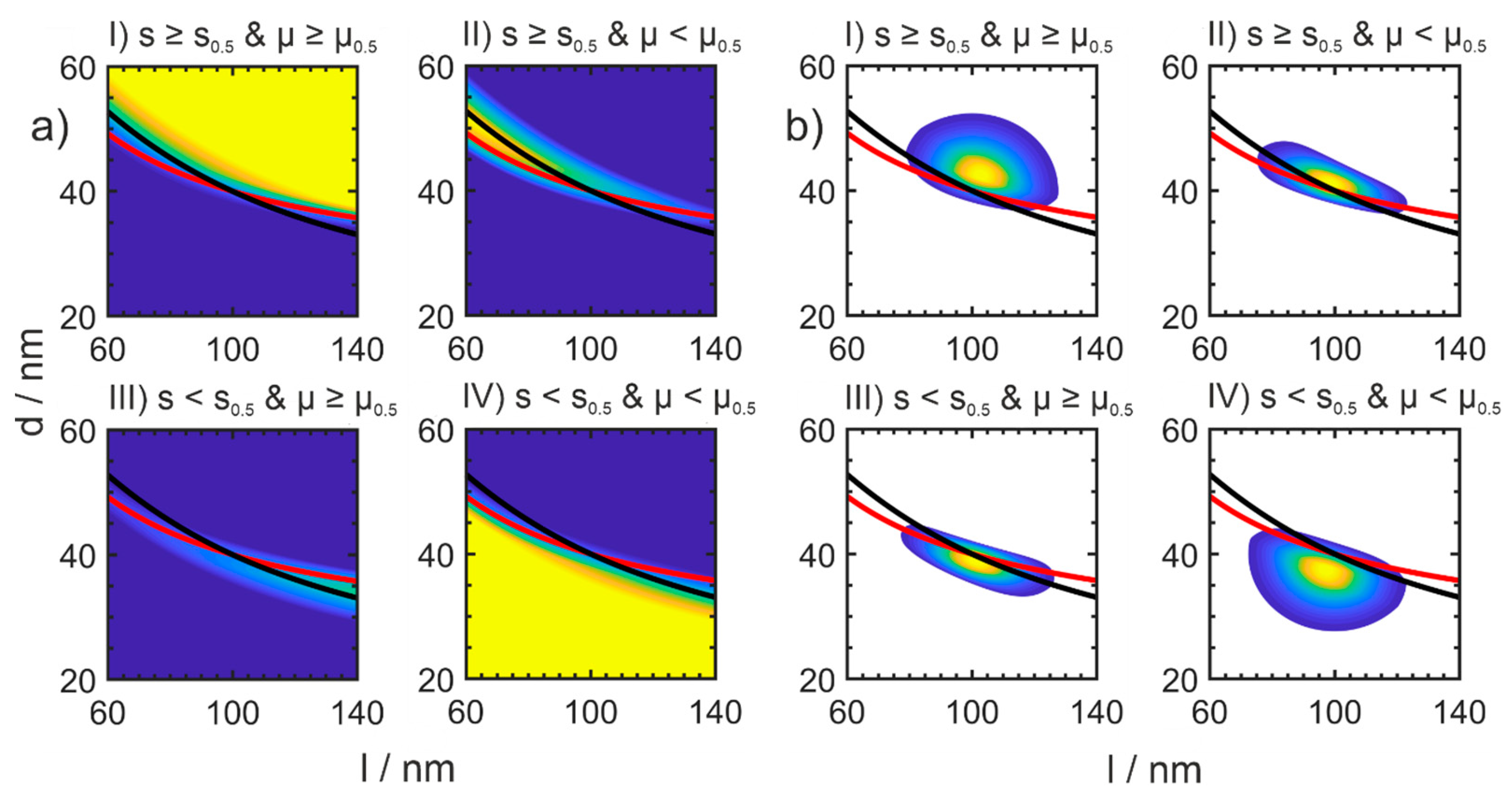
Figure 9.
Decoupled consecutive separations with orthogonal force separation corresponding to consecutive separation.
Figure 9.
Decoupled consecutive separations with orthogonal force separation corresponding to consecutive separation.

Figure 10.
Sketch of a hydrocyclone with characteristic dimensions.

Figure 11.
Corrected separation function T′(d, l) according to (40) for the separation of silica spheres and plates (a). Dashed lines show lines of the same volume (cylinders). Number-based particle size distributions for silica spheres and platelets of the feed (b), the fine fraction (c) and the coarse fraction (d). Dashed lines show the T25 and T75, solid line the T50.
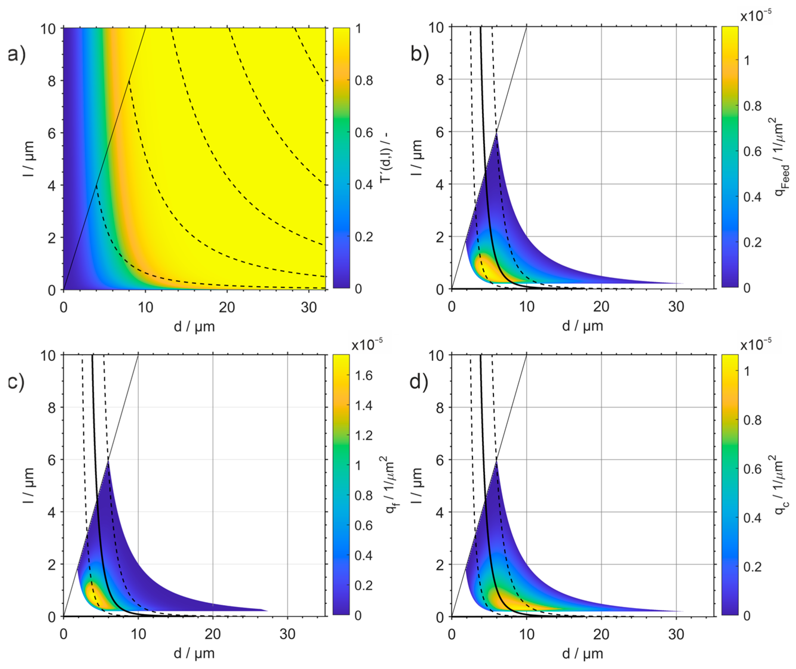
Figure 12.
Sketch of a plate separator. Reproduced with permission from [44]. Copyright 2023, Elsevier.
Figure 12.
Sketch of a plate separator. Reproduced with permission from [44]. Copyright 2023, Elsevier.
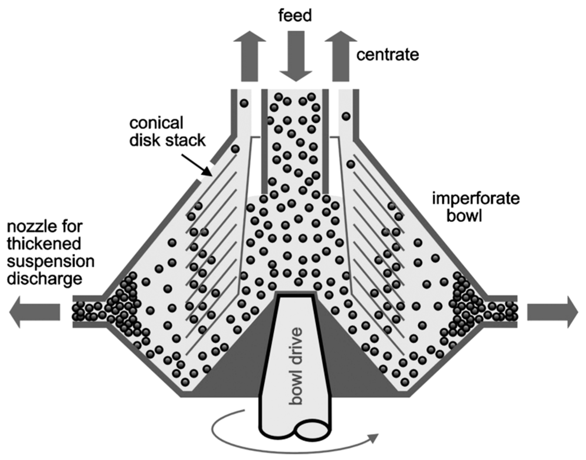
Figure 13.
Size and density distribution of the feed dispersion (a), calculated 2D separation function (b), size and density distribution of coarse (c) and fine (d) fraction after classification with the disc separator.
Figure 13.
Size and density distribution of the feed dispersion (a), calculated 2D separation function (b), size and density distribution of coarse (c) and fine (d) fraction after classification with the disc separator.

Disclaimer/Publisher’s Note: The statements, opinions and data contained in all publications are solely those of the individual author(s) and contributor(s) and not of MDPI and/or the editor(s). MDPI and/or the editor(s) disclaim responsibility for any injury to people or property resulting from any ideas, methods, instructions or products referred to in the content. |
© 2023 by the authors. Licensee MDPI, Basel, Switzerland. This article is an open access article distributed under the terms and conditions of the Creative Commons Attribution (CC BY) license (https://creativecommons.org/licenses/by/4.0/).
Share and Cite
MDPI and ACS Style
Frank, U.; Dienstbier, J.; Tischer, F.; Wawra, S.E.; Gromotka, L.; Walter, J.; Liers, F.; Peukert, W. Multidimensional Fractionation of Particles. Separations 2023, 10, 252. https://doi.org/10.3390/separations10040252
AMA Style
Frank U, Dienstbier J, Tischer F, Wawra SE, Gromotka L, Walter J, Liers F, Peukert W. Multidimensional Fractionation of Particles. Separations. 2023; 10(4):252. https://doi.org/10.3390/separations10040252
Chicago/Turabian StyleFrank, Uwe, Jana Dienstbier, Florentin Tischer, Simon E. Wawra, Lukas Gromotka, Johannes Walter, Frauke Liers, and Wolfgang Peukert. 2023. "Multidimensional Fractionation of Particles" Separations 10, no. 4: 252. https://doi.org/10.3390/separations10040252
Note that from the first issue of 2016, this journal uses article numbers instead of page numbers. See further details here.