Development of a Combined Heart-Cut and Comprehensive Two-Dimensional Gas Chromatography System to Extend the Carbon Range of Volatile Organic Compounds Analysis in a Single Instrument

Abstract

The majority of atmospheric measurements of volatile organic compounds (VOCs) are usually limited to a small range, either in volatility or time resolution. A combined heart-cut gas chromatography (GC) with comprehensive two-dimensional GC (GC×GC) instrument was developed, specifically to increase the number of VOCs analysed using a single instrument. The system uses valve based modulation and was fully automated, making it suitable for use in the field. A laboratory comparison to an existing dual-channel GC (DC-GC) instrument demonstrated that this new GC-GC×GC can accurately measure atmospheric mixing ratios of C${}_5$-C${}_{13}$ VOC species with a wide range of functionalities. Approximately hourly field measurements were conducted at a remote marine atmospheric research station in Bachok, Malaysia. This region was shown to be influenced by clean marine air masses, local anthropogenic and biogenic emission sources and aged emissions transported from highly polluted South East Asian regions. A dramatic shift in air mass direction was observed each day associated with the development of a sea breeze, which influenced the diurnal profiles of species measured at the Bachok site. A proton-transfer-reaction mass spectrometer (PTR-MS) was also deployed at Bachok and compared to the new GC-GC×GC instrument. Overall, the GC-GC×GC instrument has been shown to perform well in lab comparisons and during field observations. This represents a good compromise between volatility and high complexity $online$ measurements of VOCs.

1. Introduction

Volatile organic compounds (VOCs) play a central role in the atmosphere through reactions which can produce secondary pollutants such as secondary organic aerosol (SOA) and ozone (O${}_3$), both of which are detrimental to health. Atmospheric VOC measurements generally fall into one of two categories; $offline$, where the sample is collected and analysed back at the laboratory, or $online$, where the instrument is deployed to the field. There are a variety of instruments designed to measure the atmospheric concentrations of VOCs. One of the most common methods of VOC analysis, both off and online, is thermal desorption gas chromatography coupled to either a flame ionisation detector or mass spectrometer (TD-GC-FID/MS) [1].

The majority of online, longer term atmospheric VOC measurements span a range of C${}_2$-C${}_8$ hydrocarbons; including alkanes, alkenes and simple aromatic compounds such as benzene, toluene and xylenes. This select group of VOCs are routinely measured in many countries for compliance with air quality policy, however there are potentially many thousands of VOC compounds that are not routinely measured and as a result their influence on local processes and secondary pollution generation is not well established. The complexity is further complicated by the exponential increase in structural isomers with increasing carbon number [2].

Measurement of higher carbon number VOCs in the atmosphere is much rarer than small chain hydrocarbons. Our previous measurement approach, detailed in Dunmore et al. (2015), used comprehensive two-dimensional GC (GC×GC) [3], a method that can increase the number of VOC species identified in complex mixtures, such as urban air, when compared to single column GC [4]. GC×GC instruments subject the entire sample under analysis to a separation in two dimensions through the use of two GC columns connected via a modulator. The modulator fractionates the eluent from the primary column and injects it onto the secondary column at rapid, regular time intervals. The secondary column subjects the sample to a fast separation, typically less than 10 s, prior to the next modulation. This combination of two GC columns with different selectivities improves the separation and resolution power of the instrument and is particularly effective at resolving compounds with similar boiling points but different polarities [5].

During the Clean air for London (ClearfLo) campaign of 2012 (detailed in Bohnenstengel et al. (2014) [6] and Dunmore et al. (2015) [3]), the original GC×GC instrument was unable to fully separate, and therefore quantify, isoprene from the band of other aliphatic compounds in the chromatogram (shown in Appendix Figure A1). This is likely a direct result of using a narrow primary BPX-5 column (0.15 mm), needed for the valve based GC×GC system, but does lead to a more limited separation of the most volatile VOC species. A Dual Channel (DC)-GC instrument (described in Hopkins et al. (2011) [7]) was also deployed during the ClearfLo campaign, which could accurately and reliable quantify isoprene, and other C${}_2$-C${}_8$ VOCs allowing an extensive characterisation of the VOC mix in urban air.

Isoprene has been shown to be extremely important in tropical regions, particularly those with forested areas [8] meaning that the existing GC×GC method missed a vital VOC. The overall aim of this development was to extend the carbon range of VOCs that could be quantified using a single instrument. In particular, obtaining both an accurate and reproducible measure of isoprene in addition to maintaining the separation of larger carbon number species was a key goal of this research.

The coupling of either multiple GC techniques or detectors into a hyphenated system can provide a superior method to studying complex samples, such as the VOC composition of the atmosphere [9], These systems could be a combination of one dimensional (1D) GC, heart-cut GC (GC-GC) and/or GC×GC in a single instrument that can be implemented to provide the best resolution and separation of a sample [9]. Multi-dimensional GC systems are typically comprised of GC-GC, where targeted and discrete sections of the 1D column separation are transferred either for further separation on a second dimension (2D) and/or to a different detection system [9,10]. The columns are connected through the use of either a switching valve or pressure-driven switching device [11]. The targeted regions are subjected to a greater separation than would be possible using 1D GC alone [9].

This paper details the development of a new combined heart-cut and GC×GC instrument (GC-GC×GC) to measure a wider range of VOCs. There are several methods that could have been used to optimise the original GC×GC instrument; for example, changing the modulation parameters, introducing a secondary oven, changing the detector from an FID to MS etc. The latter however, would have made the instrument less portable than with an FID. Ideally, this new instrument should be as close to the original design as possible but still be field portable to very remote locations. A well established and validated DC-GC instrument was able to quantify several high volatility VOCs, specifically isoprene thus the setup of this instrument was used to inform the design of the new GC-GC×GC. This new instrument was then compared to the DC-GC described in Hopkins et al. (2011) [7]. The GC-GC×GC instrument was deployed at a newly developed research facility located at the University of Malaya Bachok Marine Research Station (BMRS). The campaign during January and February 2014 was designed to investigate the composition of air flowing from industrialised regions to the north of the South China Sea.

Bachok, Malaysia is at the centre of an important region of the globe, often referred to as the Maritime Continent (MC) in South East Asia which comprises many islands, peninsulas and shallow seas between approximately 10${}^{\circ }$ S to 20${}^{\circ }$ N and 90 to 150${}^{\circ }$ E. This region is subject to a complex mix of anthropogenic and biogenic emissions including; industrial emissions from the rapidly-developing nations in Asia (particularly the south east), biomass burning emissions from tropical forests, and emissions from natural and cultivated terrestrial and marine ecosystems. The large scale transport of atmospheric species in this region is controlled by the oscillation of the intertropical convergence zone and the accompanying monsoon seasons. Of particular interest during the winter months, is the flow of air from highly industrialised and populated regions in China, Japan, Korea and Taiwan over the South China Sea. This, in conjunction with the increasing anthropogenic emissions from these countries, due to the rapid development they are undergoing, could be potentially significant when considering regional radiative forcing. Even though this region is of high interest, there have so far been a limited number of studies conducted.

2. Materials and Methods

The GC-GC×GC system comprised of an Agilent 7890 GC with two FIDs operating at 200 Hz (Agilent Technologies, Wilmington, DE, USA). The FIDs were both heated to 300 ${}^{\circ }\mathrm{C}$, with 30 mL·min${}^{-1}$ hydrogen and 300 mL·min${}^{-1}$ compressed air, (provided by generators in the laboratory and cylinders in the field). This system is made up of three columns: the GC×GC stage used a primary BPX-5 column (25 m, 0.15 mm, 0.4 $\mathsf{\mu }$m, SGE Analytical Science, Victoria, Australia; column pressure of 60 psi) and a secondary BP-20 column (5 m, 0.25 mm, 0.25 $\mathsf{\mu }$m, SGE Analytical Science; 23 psi), and the heart-cut stage used a secondary aluminium oxide Porous Layer Open Tubular (PLOT, 25 m, 0.25 mm, 0.4 $\mathsf{\mu }$m, Agilent Technologies, Edinburgh, UK; 11 psi) column. The columns used constant pressure throughout the GC run, with helium as the carrier gas (provided by cylinders of CP grade equivalents in both the laboratory and in the field). Two 4-port, 2-way valves (Valco Instruments, Houston, TX, USA) were used to switch between the heart-cut and GC×GC stages. A 6-port, 2-way diaphragm valve (Valco Instruments) was used as the total transfer flow modulator for the GC×GC stage. The modulator was held at 100 ${}^{\circ }\mathrm{C}$ throughout the run and had a modulation period of 5 s (comprised of a 4.7 s sample and 0.3 s injection periods).

Thermal desorption of ambient samples was achieved using a Markes TT24-7 unit with an air server attachment (Markes International, Llantrisant, UK), sampling at a rate of 100 mL·min${}^{-1}$ for 55 min, to give a total sample volume of 5.5 L. The trapping temperature was set at −10 ${}^{\circ }\mathrm{C}$, and then heated to 200 ${}^{\circ }\mathrm{C}$ at 100 ${}^{\circ }\mathrm{C}$·min${}^{-1}$ (maximum temperature held for 3 min, combined trap desorption time of 5 min) to desorb all analytes of interest.

During an intercomparison phase, outside air was sampled from a manifold attached to the roof of the Wolfson Atmospheric Chemistry Laboratory based on the University of York, Heslington West campus. Air samples were pumped through a glass finger in an ethylene glycol bath held at −30 ${}^{\circ }\mathrm{C}$, to remove any moisture present. An oven temperature programme for the GC-GC×GC instrument was developed to optimise the separation and resolution of analytes. The initial temperature was 50 ${}^{\circ }\mathrm{C}$, held for 3 min, ramped at 2.5 ${}^{\circ }\mathrm{C}$·min${}^{-1}$ to 130 ${}^{\circ }\mathrm{C}$, held for 2 min then ramped at 10 ${}^{\circ }$$\mathrm{C}$·min${}^{-1}$ to 200 ${}^{\circ }\mathrm{C}$, and held for 6 min; giving a total run time of 50 min. The total analysis time was 55 min.

The GC-GC×GC instrument developed was compared to a well-established DC-GC that is operated by the National Centre for Atmospheric Science (NCAS) Atmospheric Measurements Facility. A detailed reporting of the DC-GC set up and calibration is provided by Hopkins et al. (2003) [12]. Briefly, this instrument has two GC columns; an aluminium oxide PLOT column and a LOWOX column for the analysis of VOCs and oxygenated VOCs (OVOCs) respectively.

2.1. Bachok Demonstration ‘International Opportunities Fund’ Campaign

The GC-GC×GC was deployed at the University of Malaya BMRS, located on the eastern coast of Peninsular Malaysia, within 100 m of the South China Sea (6${}^{\circ }$0’31.878”N, 102${}^{\circ }$25’49.2672”E). This site is owned and operated by the University of Malaya (UM) as part of the Institute of Ocean and Earth Sciences (IOES). The intensive demonstration activity ran from st 21 January until th 6 February 2014, was funded by the National Environment Research Council and the UM and involved several UK universities (Universities of East Anglia, Cambridge, York, Leeds, Leicester and Royal Holloway University of London), NCAS, UM and Met Malaysia. Measurements were taken from the top of an atmospheric observation tower (7 floors, ≈ 15 m) on the beach side of the site, using the GC-GC×GC method described in the previous section. The gases used during this sampling period were from cylinders at the same purity as previously described.

2.2. Compound Identification and Quantification

Individual VOC compounds were identified and quantified using either a certified gas standard or using retention indices from liquid standards. The certified gas standard contained 30 ozone precursor VOC compounds (C${}_2$-C${}_9$, NPL 30, National Physical Laboratory, Teddington, UK) at 3–5 ppb levels. This was used at regular intervals both in the laboratory and in the field based study to perform gas phase calibrations. Compounds not included in the gas standard were identified and quantified using splitless injections from liquid standards. This was discussed in detail in the Supplementary Information, Section 1.3 of Dunmore et al. (2015) [3]. The data processing and integration was done using ChemStation (Agilent Technologies) for the 1D GC data and Zoex GC image (Zoex, Houston, TX, USA) for the 2D GC data.

2.3. Supporting Measurements

Measurements of nitric oxide (NO) and nitrogen dioxide (NO${}_2$) were performed using a two channel TE42i commercial gas analyser (Thermo Scientific, Waltham, MA, USA) which utilises the chemiluminescence produced by the reaction between NO and ozone (O${}_3$). Measurements are made alternately using a single reaction chamber with an upstream solenoid to select between NO and NO${}_2$, where the NO${}_2$ is converted to NO using a molybdenum convertor operated at 350 ${}^{\circ }\mathrm{C}$. Due to the high non-selectivity of the molybdenum convertor the NO${}_2$ measurement can be positively biased due to the conversion of other reactive nitrogen compounds (i.e., Peroxyacyl nitrates, alkyl nitrates and nitric acid) to NO. Calibration was routinely performed with a 1 ppm NO reference gas standard certified with an accuracy of ± 1 percent (Alpha gas standard, BOC Industrial Gases, Surrey, UK).

3. Results and Discussion

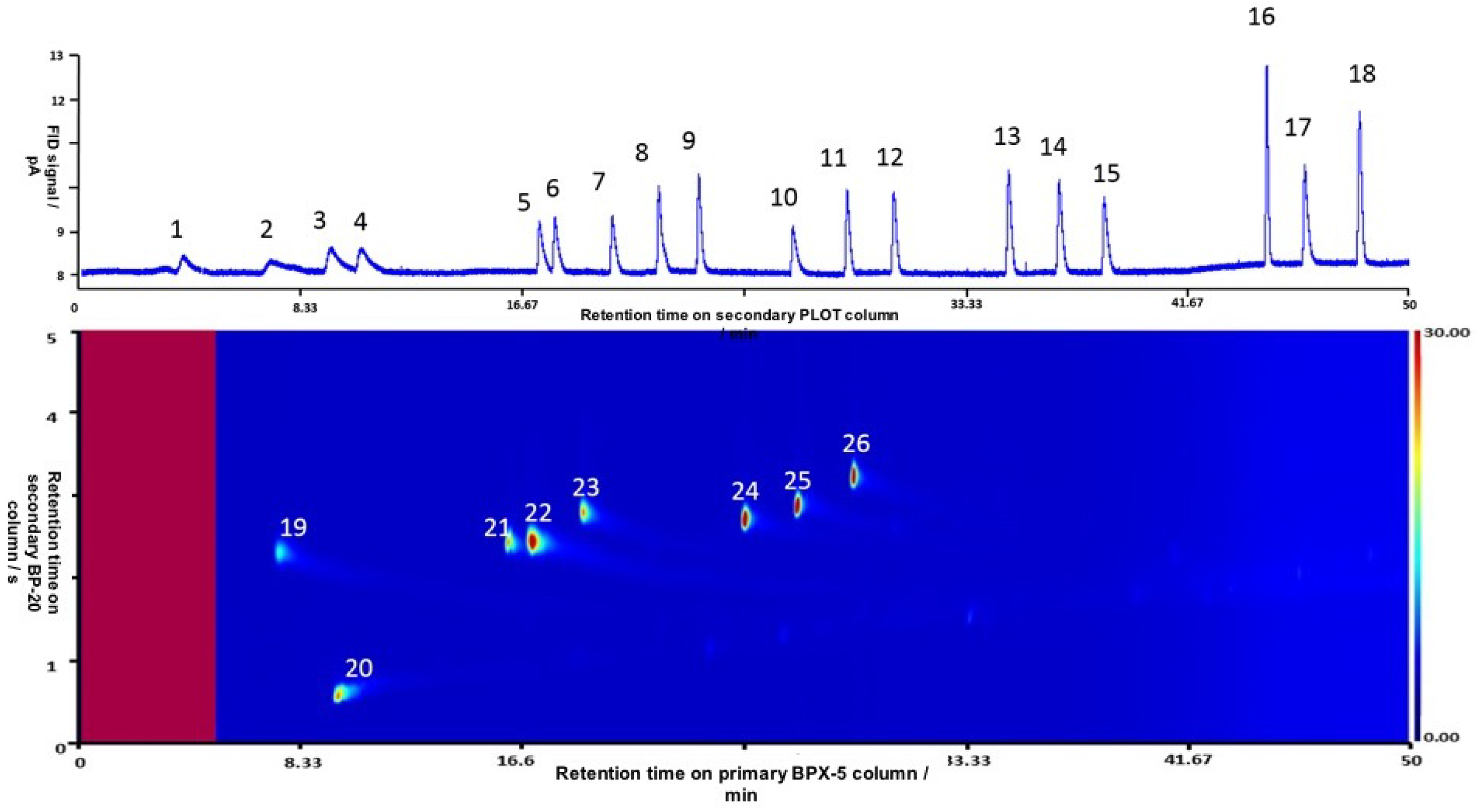
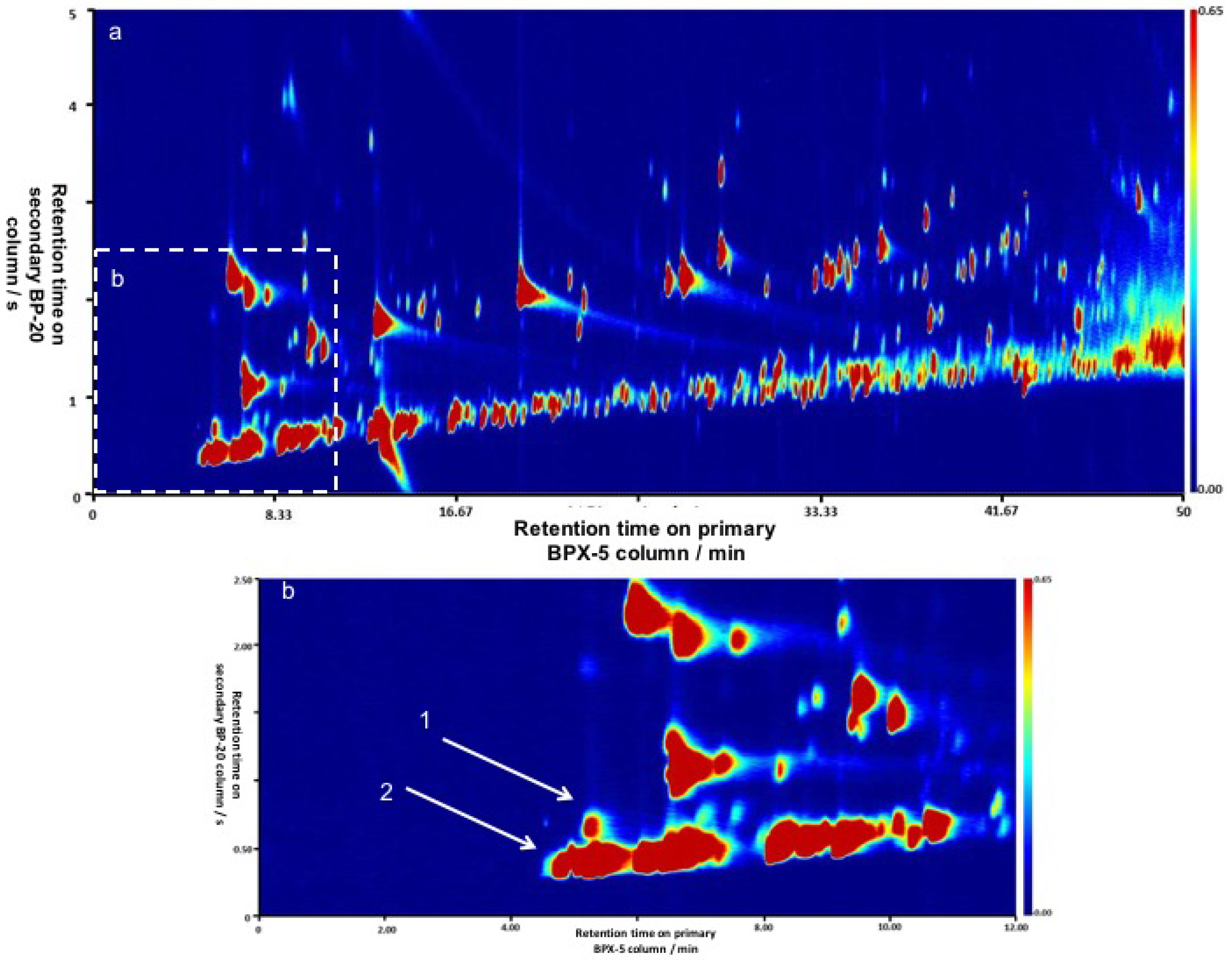
3.1. Development of the GC-GC×GC

The GC-GC×GC instrument had two operating modes, a volatile heart-cut stage (GC-, first 5 min) and a normal GC×GC stage (5 to 50 min) as shown in Figure 1. For the heart-cut stage, eluent was directed down the primary BPX-5 column, through valves 1 and 2, onto a secondary PLOT column coupled to FID 1. After 5 min, the valves switch position and the secondary PLOT column was supplied with an auxiliary helium flow of 11 psi. The heart-cut stage essentially acts to inject the most volatile VOCs (C${}_4$-C${}_7$), which are unretained by the primary BPX-5 column, onto the secondary PLOT column. For the rest of the duty cycle, these volatile species are separated on the secondary PLOT column. The remainder of the VOCs (C${}_8$-C${}_{13}$) are separated in the GC×GC stage, where eluent from the primary BPX-5 column is modulated using the total transfer flow valve modulator. The secondary BP-20 column was connected to FID 2 for detection.

One of the issues encountered when sampling ambient air using a thermal desorption unit and injecting onto a relatively narrow primary BPX-5 column (0.15 mm) was a high degree of band broadening, ultimately resulting in poor chromatographic resolution. A cryogenic (cryo)-focusing step was introduced after the TDU, to allow for the sample to be re-focused and held at the front of the primary BPX-5 column prior to separation, as shown in Figure 2a. Turning off the cryogen allowed the sample to be injected as a narrow plug. To make this step suitable for field work, a re-focusing T-piece (SGE Analytical Science) was used in conjunction with a cylinder of liquid CO₂ [13]. As shown in Figure 2a, the primary BPX-5 column is threaded through the T-piece and liquid CO₂ was sprayed around the column during sample injection activated by a solenoid. In order for the trapped analytes to be released, the T-piece was housed within the GC oven to allow rapid temperature equilibration after the cryogen was switched off.

Duplicate injections were run using an $in-house$ produced toluene gas cylinder at 26 ppbv to investigate the effects of cryo re-focusing on the separation in the first and second dimensions during GC×GC analysis. When the cryo re-focusing was on, the toluene peak was much narrower in the first dimension, with only 6 modulated peaks (Figure 2e) as opposed to over 16 without re-focusing (Figure 2d). The first dimension retention time was also slightly increased as a result of the re-focusing process.

The optimum re-focusing time was investigated by changing the cryo re-focusing time period from 0 s to 120 s at 30 s increments. For compounds which are weakly retained, a cryo-focusing period of over 60 s results in progressively more band broadening. Conversely, for strongly retained compounds, there was no significant amount of re-focusing until 120 s. However with longer time periods, the T-piece became blocked with ice, which reduced the efficiency of the re-focusing step. A 60 s time period was found to be optimum, with reduced peak widths and little distortion of the peak shapes.

Figure 3 shows the chromatogram of the 30 ozone precursor VOC compound gas standard (NPL 30) obtained using the GC-GC×GC instrument. Of the 30 VOC compounds in this standard, 27 were fully separated and quantified although m- and p-xylene were identified as one as they co-eluted. The three compounds not separated are ethane, ethene, and propene due to the very small carbon numbers, and low boiling points of these compounds. The upper panel shows the 1D GC-FID chromatogram, where the x-axis is retention time on the secondary PLOT column and the y-axis is peak amplitude. The lower panel shows the GC×GC-FID chromatogram in the form of a contour plot, where the x and y-axis are the retention times on the primary BPX-5 (separation based on boiling point) and secondary BP-20 (based on polarity) columns respectively and the coloured contour is peak intensity. The red section at the start of the chromatogram is indicative of the first 5 min of the run when the system was in heart-cut mode, such that no GC×GC separation occurs. This chromatogram shows good separation of the species of interest and the ability to separate and resolve isoprene. The 1D GC-FID chromatogram (upper panel) contains hydrocarbons from C₃-C₇, inclusive of isoprene and benzene, while the GC×GC contour plot (lower panel) consists of higher carbon number species (C₇-C₁₃); such as larger aromatics and aliphatics, along with other functional groups.

The use of online sorbent tube sampling via a thermal desorption unit is a common practice for in-situ field campaigns, however it is essential that breakthrough tests are carried out to test the validity of the method to sample ambient air. Breakthrough tests are used to determine what parameters should be maintained to ensure that none of the analyte of interest was lost or undetected [14]. If not carried out the wrong sampling volume may be used, i.e., too high a volume could cause the sorbent to become saturated with analyte leading to a false quantification.

To test the sorbent tubes used, a set of serial dilutions were conducted using the 30 component VOC gas standard (NPL 30). A particular focus of this testing was to determine the linearity of the calibration for the more volatile compounds being targeted by the new set-up (i.e., C₃-C₆) over a range of mixing ratios from 0.4 to 4 ppbv. The results of these tests showed that this method was not suitable for the analysis of species with 4 or less carbon atoms but gave a linear response for isoprene, the specific target compound of interest, at expected atmospheric mixing ratios (shown in

Table 1. Gradient, intercepts and R${}^2$ values for breakthrough test compounds. Numbers correspond to the identified peaks in Figure 3, acetylene and $cis$-2-pentene are not included.

	Compounds	Gradient	Intercept/10${}^{-15}$	R${}^2$
1	n-Propane	−1.5010	4.1427	0.15
2	$iso$-Butane	−1.8479	4.5295	0.17
3	n-Butane	−0.3147	4.5533	0.58
5	$trans$-2-Butene	0.0995	−0.7799	0.81
6	1-Butene	0.1419	−1.0857	0.69
7	$cis$-Butene	0.0937	−0.7115	0.83
8	$iso$-Pentane	0.0916	−0.9669	0.87
9	n-Pentane	0.0368	−0.0771	0.99
10	1,3-Butadiene	0.0654	0.2000	0.43
11	$trans$-2-Pentene	0.0393	−0.0736	0.99
13	2/3-methyl Pentane	0.0322	−0.1313	0.99
14	n-Hexane	0.0302	−0.0658	0.99
15	Isoprene	0.0397	−0.0623	0.99
16	n-Heptane	0.0264	−0.0751	0.99
17	Benzene	0.0312	−0.0910	0.99
18	2,2,4-trimethyl-Pentane	0.0231	−0.0602	0.99

).

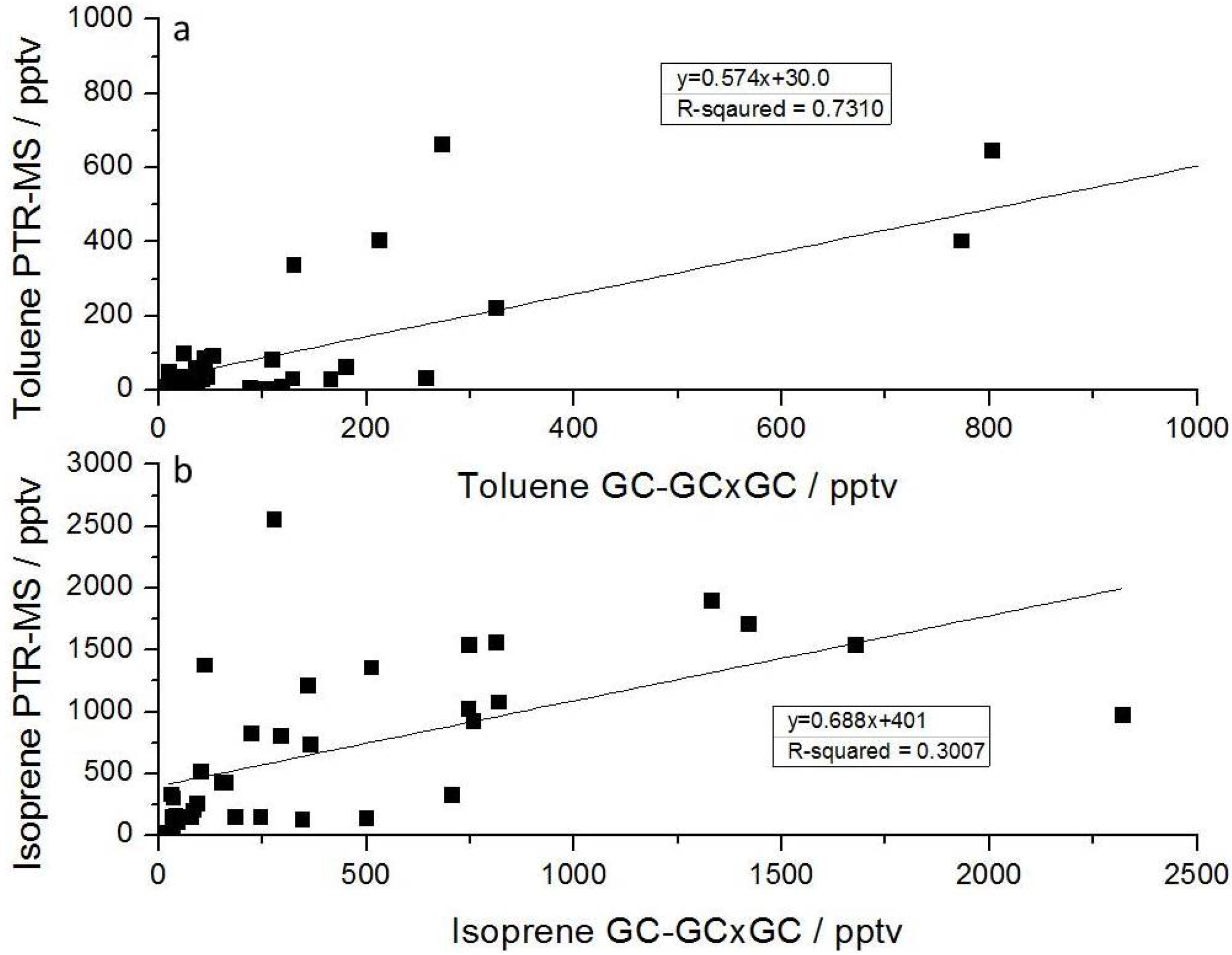
3.2. Comparison of GC-GC×GC with an Established DC-GC

By comparing this new GC-GC×GC instrument against a well established DC-GC instrument [7], its performance was evaluated. The two instruments both observed 27 of the compounds in the 30 component VOC gas standard (i.e., those shown in Figure 3 with m- and p-xylene identified as one compound). The measured atmospheric mixing ratios of two of the compounds, n-pentane and isoprene, observed in York by both instruments, are shown in Figure 4. These two compounds were chosen to show whether the new GC-GC×GC instrument can accurately observe the target compound, isoprene, and n-pentane another more volatile VOC than the previous GC×GC setup could observe. The two instruments compare very well for both compounds, (with linear regression correlations of R${}^2$ of 0.992 for n-pentane and R${}^2$ of 0.997 for isoprene). There are some discrepancies between the techniques, towards the end of the n-pentane time series. This analysis was carried out at the Department of Chemistry, University of York so it was likely emissions of n-pentane from solvent use in the department may be influencing the time series. The two instruments also have very different sampling methods which may be another reason for this discrepancy. The DC-GC instrument samples for 10 min and runs the sample for 50 min, while the GC-GC×GC instrument continuously samples for 55 min and runs for 50 min. Therefore the two instruments will observe different mixing ratios, especially when concentrations are changing rapidly.

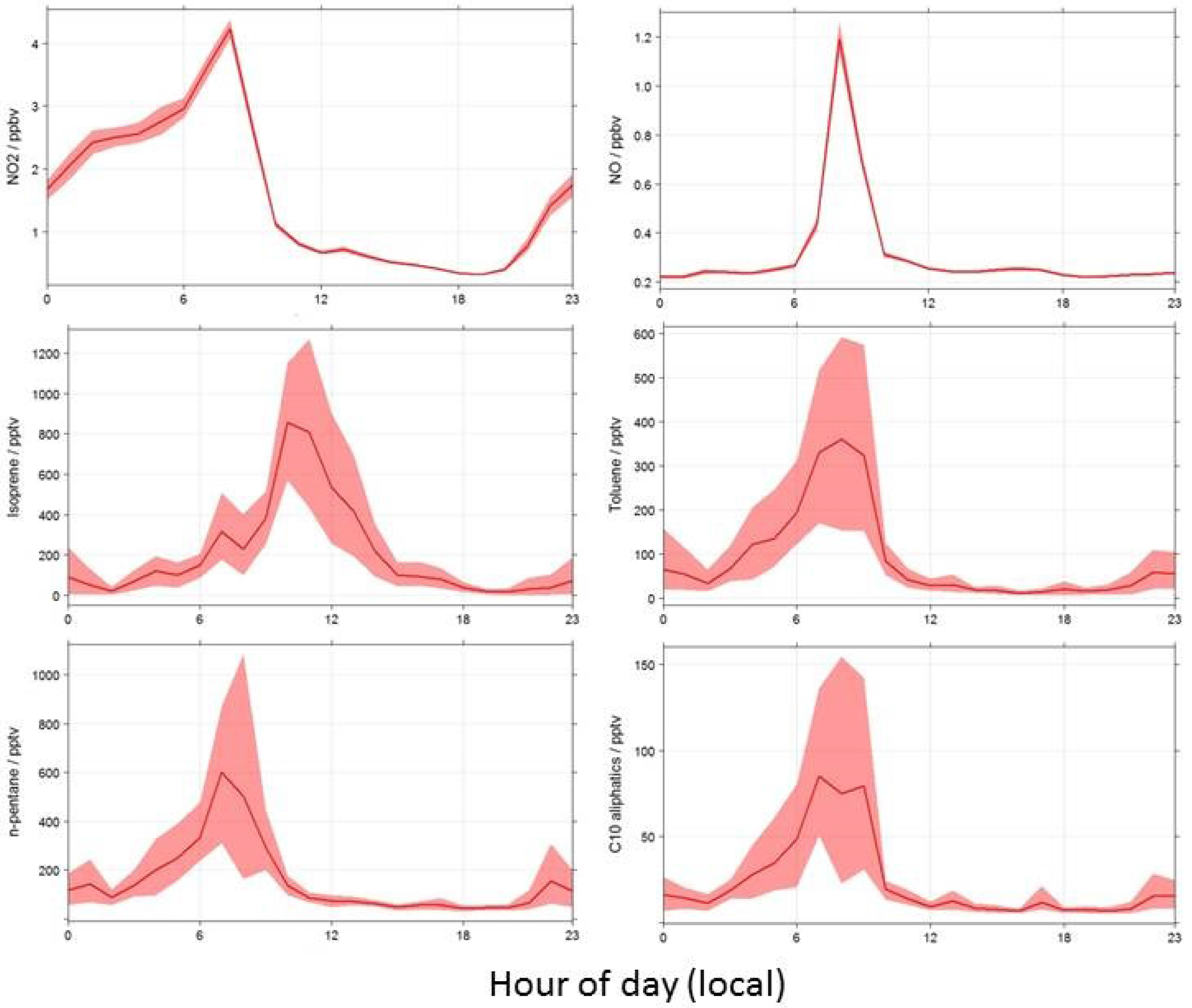
3.3. Bachok Demonstration ‘International Opportunities Fund’ campaign

The GC-GC×GC instrument was deployed to Bachok and a sample chromatogram from 22:32 (local time) on 01/02/2014 is shown in Figure 5. This figure shows the 1D GC chromatogram in the upper panel (a), the GC×GC chromatogram in the middle panel (b) and a zoomed in section of the 1D GC chromatogram in the lower panel (c, indicated by the dashed box in panel a). The combination of the 1D GC chromatogram and the 2D GC contour plot shows the presence of approximately a hundred individual VOC species in the atmosphere. A selection of individual and grouped VOCs are identified in Figure 5 to show the breadth of species that can be quantified. The zoomed in section of the 1D GC chromatogram (c in Figure 5) shows that, although the chromatogram is dominated by one thus far unidentified compound, there are also many other VOCs with less than 7 carbon atoms present at low mixing ratios. From Figure 5b, it appears that there was some co-elution with toluene and another VOC compound. This other compound has not been positively identified however was taken into account during quantification.

Figure 6 shows the average diurnal profiles observed during the entire measurement period at Bachok for selected VOCs, nitrogen oxide (NO) and nitrogen dioxide (NO₂). The profiles of NO and the anthropogenic VOCs (toluene, n-pentane and C₁₀ aliphatics) show a morning peak at approximately 07:00, with a sharp decrease seen around 10:00 where the concentrations are sustained at a minimum until the next morning. NO₂ shows a similar profile, except that it begins to increase from ≈ 20:00 to the maximum early in the morning (≈ 08:00). The diurnal profile of isoprene shows a maximum just before midday that is not present in the profiles of the anthropogenic VOCs, consistent with the presence of an overwhelming biogenic source that is driven by solar intensity. However, the profile still drops off faster than expected as a result of a switch in wind direction most days at approximately midday as a sea breeze developed. During the morning hours, the air being sampled was coming over the land and showed very high levels of NO, NO₂ and the anthropogenic VOCs. The sources of these were likely local small scale open burning of primarily household refuse, seen by the peaks in all species at approximately 08:00. When the wind direction changes, a rapid decrease in concentration was observed, particularly in the profiles of NO, NO2 and anthropogenic VOCs.

During the Bachok demonstration campaign, the University of East Anglia also measured VOCs using a PTR-MS (instrument details are described in Murphy et al. (2010) [18]). Some of these species overlapped with those measured using the GC-GC×GC instrument. During periods where both instruments were operational, similar trends and profiles were observed, though the PTR-MS produced more structured data due to its faster time resolution (approximately minute data, compared to almost hourly data from the GC-GC×GC), shown in Figure 7. Both instruments observed the sharp decrease prior to midday for the anthropogenic VOCs, assumed to be when the wind direction changed from land to marine influenced air masses as a result of the sea breeze. The PTR-MS did show significantly higher observed mixing ratios of isoprene than the GC-GC×GC instrument (Figure 7c,d). This may be due to interferences from furan, which could also appear at the same m/z channel as isoprene. This is evident in the linear regression correlation plot for isoprene (Figure 8b) which has a high intercept (+401 pptv) on the line of best fit for the PTR-MS. In contrast, the linear regression correlation for toluene from both instruments shows that they compare quite well, (R${}^2$ of 0.7310), and there is only a very small offset (+30 pptv) in the intercept which could be due to calibration bias or from differences in time resolution.

4. Conclusions

The GC×GC instrument detailed in Dunmore et al. (2015) [3] performed well for the majority of compounds, however it was unable to accurately quantify isoprene due to the incomplete separation and resolution of the species from surrounding compounds. Combining heartcut 1D GC with GC×GC has allowed the range of VOCs quantified to be extended using a single, field deployable instrument (GC-GC×GC) and provides a method that can accurately quantify isoprene. Comparison to an existing instrument demonstrated that this new GC-GC×GC can accurately measure C₅-C₁₃ VOC species with a wide range of functionalities. Approximately hourly measurements were conducted in a remote environment, Bachok, Malaysia. This region was shown to be influenced by marine air masses, local anthropogenic and biogenic emission sources and transported emissions from across highly polluted regions. There appears to be a dramatic shift in air mass direction each day, which has been shown to influence the diurnal profiles of species measured at the Bachok site. A PTR-MS was also deployed to Bachok and the two instruments compared well. The linear regression correlation between the two instruments for isoprene was shown to be rather poor ((R${}^2$ of 0.3007), likely from integer mass interference on the PTR-MS. This was not seen with other compounds that both instruments measured, such as toluene (R${}^2$ of 0.7310). Overall, this new GC-GC×GC instrument has been shown to perform well in lab comparisons and in situ operation. This instrument has the potential to expand the range of VOCs that can be observed in remote, hard to access regions to provide a more detailed characterisation of the atmospheric VOC loading. It may be possible to use this instrument in other research areas as well such as, fragrance, breath, or indoor air monitoring.

References

1. Singh, H. Guidance for the Collection and Use of Ambient Hydrocarbon Species Data in Development of Ozone Control Strategies; U.S. Environment Protection Agency, EPA 450/4-80-008: 1980. Available online: http://nepis.epa.gov/Exe/ZyNET.exe/91010WPX.TXT?ZyActionD=ZyDocument&Client=EPA&Index=1976+Thru+1980&Docs=&Query=&Time=&EndTime=&SearchMethod=1&TocRestrict=n&Toc=&TocEntry=&QField=&QFieldYear=&QFieldMonth=&QFieldDay=&IntQFieldOp=0&ExtQFieldOp=0&XmlQuery=&File=D%3A%5Czyfiles%5CIndex%20Data%5C76thru80%5CTxt%5C00000021%5C91010WPX.txt&User=ANONYMOUS&Password=anonymous&SortMethod=h%7C-&MaximumDocuments=1&FuzzyDegree=0&ImageQuality=r75g8/r75g8/x150y150g16/i425&Display=p%7Cf&DefSeekPage=x&SearchBack=ZyActionL&Back=ZyActionS&BackDesc=Results%20page&MaximumPages=1&ZyEntry=1&SeekPage=x&ZyPURL (accessed on 1 June 2016).
2. Goldstein, A.; Galbally, I. Known and unexplored organic constituents in the Earth’s atmosphere. Environ. Sci. Technol. 2007, 41, 1514–1521. [Google Scholar] [CrossRef] [PubMed]
3. Dunmore, R.; Hopkins, J.; Lidster, R.; Lee, J.; Evans, M.; Rickard, A.; Lewis, A.; Hamilton, J. Diesel-related hydrocarbons can dominate gas phase reactive carbon in megacities. Atmos. Chem. Phys. 2015, 15, 9983–9996. [Google Scholar] [CrossRef]
4. Amador-Munoz, O.; Marriott, P. Quantification in comprehensive two-dimensional gas chromatography and a model of quantification based on selected summed modulated peaks. J. Chromatogr. A 2008, 1184, 323–340. [Google Scholar] [CrossRef] [PubMed]
5. Kallio, M.; Jussila, M.; Rissanen, T.; Anttila, P.; Hartonen, K.; Reissell, A.; Vreuls, R.; Adahchour, M.; Hyotylainen, T. Comprehensive two-dimensional gas chromatography coupled to time-of-flight mass spectrometry in the identification of organic compounds in atmospheric aerosols from coniferous forest. J. Chromatogr. A 2006, 1125, 234–243. [Google Scholar] [CrossRef] [PubMed]
6. Bohnenstengel, S.; Belcher, S.; Aiken, A.; Allan, J.; Allen, G.; Bacak, A.; Bannan, T.; Barlow, J.; Beddows, D.; Bloss, W.; et al. Meteorology, air quality, and health in London: The ClearfLo project. Bull. Am. Meteorol. Soc. 2014. [Google Scholar] [CrossRef]
7. Hopkins, J.; Jones, C.; Lewis, A. A dual channel gas chromatograph for atmospheric analysis of volatile organic compounds including oxygenated and monoterpene compounds. J. Environ. Monit. 2011, 13, 2268–2276. [Google Scholar] [CrossRef] [PubMed]
8. Hewitt, C.; Lee, J.; MacKenzie, A.; Barkley, M.; Carslaw, N.; Carver, G.; Chappell, N.; Coe, H.; Collier, C.; Commane, R.; et al. Overview: oxidant and particle photochemical processes above a south-east Asian tropical rainforest (the OP3 project): introduction, rationale, location characteristics and tools. Atmos. Chem. Phys. 2010, 10, 169–199. [Google Scholar] [CrossRef] [Green Version]
9. Chin, S.; Eyres, G.; Marriott, P. System Design for Integrated Comprehensive and Multidimensional Gas Chromatography with Mass Spectrometry and Olfactometry. Anal. Chem. 2012, 84, 9154–9162. [Google Scholar] [CrossRef] [PubMed]
10. Maikhunthod, B.; Morrison, P.; Small, D.; Marriott, P. Development of a switchable multidimensional/ comprehensive two-dimensional gas chromatographic analytical system. J. Chromatogr. A 2010, 1217, 1522–1529. [Google Scholar] [CrossRef] [PubMed]
11. Wong, Y.; Hartmann, C.; Marriott, P. Multidimensional gas chromatography methods for bioanalytical research. Bioanalysis 2014, 6, 2461–2479. [Google Scholar] [CrossRef] [PubMed]
12. Hopkins, J.; Lewis, A.; Read, K. A two-column method for long-term monitoring of non-methane hydrocarbons (NMHCs) and oxygenated volatile organic compounds (OVOCs). J. Environ. Monit. 2003, 5, 8–13. [Google Scholar] [CrossRef] [PubMed]
13. Lidster, R.; Hamilton, J.; Lewis, A. The application of two total transfer valve modulators for comprehensive two-dimensional gas chromatography of volatile organic compounds. J. Sep. Sci. 2011, 34, 812–821. [Google Scholar] [CrossRef] [PubMed]
14. Kim, K.; Lee, M.; Szulejko, J. Simulation of the breakthrough behavior of volatile organic compounds against sorbent tube sampler as a function of concentration level and sampling volume. Anal. Chim. Acta 2014, 835, 46–55. [Google Scholar] [CrossRef] [PubMed]
15. Carslaw, D.; Ropkins, K. Openair—An R package for air quality data analysis. Environ. Model. Softw. 2012, 27–28, 52–61. [Google Scholar] [CrossRef]
16. Carslaw, D.; Ropkins, K. Openair: Open-Source Tools for the Analysis of Air Pollution Data. R package version 0.6-2. 2012. Available online: http://journal.r-project.org/archive/2012-1/RJournal 2012-1 Ropkins+Carslaw.pdf (accessed on 1 June 2016).
17. R Development Core Team. R: A Language and Environment for Statistical Computing, R Foundation for Statistical Computing; R Development Core Team: Vienna, Austria, 2012. [Google Scholar]
18. Murphy, J.; Oram, D.; Reeves, C. Measurements of volatile organic compounds over West Africa. Atmos. Chem. Phys. 2010, 10, 5281–5294. [Google Scholar] [CrossRef]
Figure 1. Gas chromatography (GC)-GC×GC schematic: (a) column flows and valve positions during the volatile heart-cut stage (first 5 min of operation); (b) column flows and valve positions during the GC×GC stage (5–50 min). TDU represents the thermal desorption unit and cryo re-focuser represents the cryogenic re-focusing unit.
Separations 03 00021 g001
Figure 2. Liquid CO2 re-focusing: (a), schematic of the T-piece, (b), injection of a 26 ppbv toluene gas sample from the GC×GC stage with cryo re-focusing off, (c), injection of a 26 ppbv toluene gas sample from the GC×GC stage with cryo re-focusing on, d and e, modulated toluene peaks in more detail.
Separations 03 00021 g002
Figure 3. Chromatogram from the GC-GC×GC instrument run with a 30 component C2-C9 VOC gas standard: upper panel is a one-dimensional GC plot from the volatile heart-cut stage and the lower panel is a two-dimensional GC plot from the GC×GC stage. Compounds are identified as follows: (1) n-propane, (2) i s o -butane, (3) n-butane, (4) acetylene, (5) t r a n s -2-butene, (6) 1-butene, (7) c i s -butene, (8) i s o -pentane, (9) n-pentane, (10) 1,3-butadiene, (11) t r a n s -2-pentene, (12) c i s -2-pentene, (13) 2+3-methyl pentane, (14) n-hexane, (15) isoprene, (16) n-heptane, (17) benzene, (18) 2,2,4-trimethyl pentane, (19) toluene, (20) n-octane, (21) ethyl benzene, (22) m + p -xylene, (23) o-xylene, (24) 1,3,5-trimethyl benzene, (25) 1,2,4-trimethyl benzene and (26) 1,2,3-trimethyl benzene.
Separations 03 00021 g003
Figure 4. Left panel: Time series of n-pentane (upper) and isoprene (lower) from the GC-GC×GC (black) and dual-channel (DC)-GC (red) instruments, right panel: Linear regression comparisons for n-pentane (upper) and isoprene (lower) (a linear regression line has been fitted to the data with the equation of the line and R 2 for each correlation shown).
Separations 03 00021 g004
Figure 5. Typical GC-GC×GC chromatogram from Bachok from 01/02/2014 at 22:32 (local time) with selected VOCs identified, (a) 1D GC chromatogram from the volatile heart-cut stage; (b) GC×GC chromatogram and (c): shows a zoomed in section of the 1D GC chromatogram, highlighted by the black dashed box in Plot a.
Separations 03 00021 g005
Figure 6. Diurnal profiles of NO, NO2, and selected volatile organic compounds (VOCs) from the GC-GC×GC instrument (isoprene, toluene, n-pentane and C10 aliphatic species), constructed using the openair project for R where the solid line represents the mean daily concentration and the shaded regions shows the 95% confidence intervals surrounding the mean [15,16,17].
Separations 03 00021 g006
Figure 7. Time series of toluene and isoprene from the proton-transfer-reaction mass spectrometer (PTR-MS) and GC-GC×GC instrument; (a) toluene from the PTR-MS; (b) toluene from the GC-GC×GC; (c) isoprene from the PTR-MS and (d) isoprene from the GC-GC×GC.
Separations 03 00021 g007
Figure 8. Linear regression comparisions for (a), toluene and (b), isoprene (a linear regression line has been fitted to the data with the equation of the line and R 2 for each correlation shown).
Separations 03 00021 g008