Positive Almost Periodic Solutions for a Delayed Predator–Prey Model with Hassell-Varley Type Functional Response

Abstract

By means of a fixed point theorem of coincidence degree theory, sufficient conditions are established for the existence of a positive almost periodic solution to a kind of delayed predator–prey model with Hassell-Varley type functional response. The method used in this paper offers a possible means to study the existence of positive almost periodic solutions to the models in biological populations. Finally, an example as well as numerical simulations are given to illustrate the feasibility and effectiveness of our results.

1. Introduction

It is well-known that the theoretical study of predator–prey systems in mathematical ecology has a long history starting with the pioneering work of Lotka and Volterra [1,2]. The principles of the Lotka-Volterra model, conservation of mass and decomposition of the rates of change in birth and death processes have remained valid until today, and many theoretical ecologists still adhere to them. This general approach has been applied to many biological systems, in particular with functional response. In population dynamics, a functional response of the predator to the prey density refers to the change in the density of prey attached per unit of time per predator as the prey density changes. During the last 10 years, there has been extensive investigation of the dynamics of predator–prey models with the different functional responses in the literature, (see [3,4,5,6,7,8,9,10,11,12,13]] and references therein).

In 1969, Hassell and Varleys [14] introduced a general predator–prey system, in which the functional response is dependent on the predator density in different ways. It is called a Hassell-Varley type functional response, which takes the following form:

$$\begin{array}{c}\hfill \left\{\begin{array}{c}{\dot{N}}_1=r{N}_1\left[1-\frac{N_1}{K}\right]-\frac{c{N}_1{N}_2}{m{N}_2^{\theta }+N_1},\hfill \\ {\dot{N}}_2=N_2\left[-d+\frac{f{N}_1}{m{N}_2^{\theta }+N_1}\right],\hfill \end{array}\right.(0<\theta <1)\end{array}$$

(1)

where θ is called the Hassell-Varley constant. In the typical predator–prey interaction where predators do not form groups, one can assume that $\theta =1$, producing the so-called ratio-dependent predator–prey system. For terrestrial predators that form a fixed number of tight groups, it is often reasonable to assume $\theta =1/2$. For aquatic predators that form a fixed number of tights groups, $\theta =1/3$ may be more appropriate. A unified mechanistic approach was provided by Cosner [16] where the Hassell-Varley functional response was derived. Hsu [16] studied System (1) and presented a systematic global qualitative analysis of it. In [17], Wang considered the following periodic predator–prey model with Hassell-Varley type functional response and time-varying delay:

$$\begin{array}{c}\hfill \left\{\begin{array}{c}{\dot{N}}_1\left(t\right)=N_1\left(t\right)\left[a\left(t\right)-b\left(t\right)N_1(t-\delta \left(t\right))-\frac{c\left(t\right)N_2\left(t\right)}{m{N}_2^{\theta }\left(t\right)+N_1\left(t\right)}\right],\hfill \\ {\dot{N}}_2\left(t\right)=N_2\left(t\right)\left[-d\left(t\right)+\frac{r\left(t\right)N_1\left(t\right)}{m{N}_2^{\theta }\left(t\right)+N_1\left(t\right)}\right],\hfill \end{array}\right.(0<\theta <1)\end{array}$$

(2)

where a, b, c, d, r and δ are nonnegative periodic functions with period T and m is a nonnegative constant. By using Mawhin’s continuation theorem of coincidence degree theory, they obtained sufficient conditions for the existence of positive periodic solutions of System (2).

In real world phenomena, the environment varies due to various factors such as the seasonal effects of weather, food supplies, mating habits and harvesting, etc. So, it is usual to assume the periodicity of parameters in the systems. However, in applications, if the various constituent components of the temporally nonuniform environment has incommensurable (nonintegral multiples, see Example 1) periods, then one has to consider the environment to be almost periodic since there is no a priori reason to expect the existence of periodic solutions. Hence, if we consider the effects of environmental factors, almost periodicity is sometimes more realistic and more general than periodicity. In recent years, the almost periodic solution of the continuous models in biological populations has been studied extensively (see [18,19,20,21,22,23,24,25] and the references cited therein).

Example 1. Let us consider the following simple population model:

$$\begin{array}{c}\hfill \dot{N}\left(t\right)=N\left(t\right)\left[|sin\left(\sqrt{2}t\right)|-|sin\left(\sqrt{3}t\right)|N\left(t\right)\right]\end{array}$$

(3)

In Equation 3, $|sin(\sqrt{2}t\left)\right|$ is $\frac{\sqrt{2}\pi }{2}$-periodic function and $|sin(\sqrt{3}t\left)\right|$ is $\frac{\sqrt{3}\pi }{3}$-periodic function, which imply that Equation (3) has incommensurable periods. Then, there is no a priori reason to expect the existence of periodic solutions of Equation (3). Thus, it is important to study the existence of almost periodic solutions to Equation (3).

Motivated by the above reason and considering that a delay may occur in the functional response of System (2), in this paper, we consider the following almost periodic predator–prey model with Hassell-Varley type functional response and time-varying delays:

$$\begin{array}{c}\hfill \left\{\begin{array}{c}{\dot{N}}_1\left(t\right)=N_1\left(t\right)\left[a\left(t\right)-b\left(t\right)N_1(t-\delta \left(t\right))-\frac{c\left(t\right)N_2(t-\tau \left(t\right))}{m{N}_2^{\theta }(t-\tau \left(t\right))+N_1\left(t\right)}\right],\hfill \\ {\dot{N}}_2\left(t\right)=N_2\left(t\right)\left[-d\left(t\right)+\frac{r\left(t\right)N_1(t-\sigma \left(t\right))}{m{N}_2^{\theta }\left(t\right)+N_1(t-\sigma \left(t\right))}\right],\hfill \end{array}\right.(0<\theta <1)\end{array}$$

(4)

where a, b, c, d, r, δ, τ and σ are nonnegative almost periodic functions and m is a nonnegative constant.

It is well known that Mawhin’s continuation theorem of coincidence degree theory is an important method to investigate the existence of positive periodic solutions to some kinds of non-linear ecosystems (see [11,12,13,26,27,28,29,30,31,32,33,34]). However, it is difficult to use it to investigate the existence of positive almost periodic solutions of non-linear ecosystems. Therefore, to the best of the author’s knowledge, so far, there have been scarcely any papers concerning the existence of positive almost periodic solutions to System (4) by using Mawhin’s continuation theorem. Motivated by the above reason, the main purpose of this paper is to establish some new sufficient conditions based on the existence of positive almost periodic solutions to System (4) by using Mawhin’s continuous theorem of coincidence degree theory.

Let $\mathbb{R}$, $\mathbb{Z}$ and ${\mathbb{N}}^{+}$ denote the sets of real numbers, integers and positive integers, respectively. Related to a continuous bounded function f, we use the following notations:

$$f^{-}=\underset{s\in \mathbb{R}}{inf}f\left(s\right),f^{+}=\underset{s\in \mathbb{R}}{sup}{f\left(s\right),\left|f\right|}_{\infty }=\underset{s\in \mathbb{R}}{sup}\left|f\left(s\right)\right|.$$

The organization of this paper is as follows. In Section 2, we make some preparations. In Section 3, by using Mawhin’s continuation theorem of coincidence degree theory, we establish some new sufficient conditions for the existence of at least one positive almost periodic solution to System (4). Two illustrative examples and numerical simulations are given in Section 4.

2. Preliminaries

Definition 1. ([35,36]) $x\in C(\mathbb{R},\mathbb{R})$ is called almost periodic, if for any $ϵ>0$, it is possible to find a real number $l=l\left(ϵ\right)>0$, for any interval with length $l\left(ϵ\right)$, there exists a number τ in this interval such that $\left|x\right(t+\tau )-x(t\left)\right|<ϵ$, $\forall t\in \mathbb{R}$. τ is called to the ϵ-almost period of x, $T(x,ϵ)$ denotes the set of ϵ-almost periods for x and l is called to the length of the inclusion interval for $T(x,ϵ)$. The collection of such functions is denoted by $AP\left(\mathbb{R}\right)$.

Lemma 1. ([35,36]) If $x\in AP\left(\mathbb{R}\right)$, then x is bounded and uniformly continuous on $\mathbb{R}$.

Lemma 2. ([35,36]) If $x\in AP\left(\mathbb{R}\right)$, then ${\int }_0^{t}x\left(s\right)\mathrm{d}s\in AP\left(\mathbb{R}\right)$ if and only if ${\int }_0^{t}x\left(s\right)\mathrm{d}s$ is bounded on $\mathbb{R}$.

Lemma 3. ([23]) Assume that $x\in AP\left(\mathbb{R}\right)\cap C^1\left(\mathbb{R}\right)$. For arbitrary interval $I=[a,b]$ with $b-a=\omega >0$, let $\xi \in [a,b]$ and $I_1=\left\{s\in [\xi ,b]:\dot{x}\left(s\right)\ge 0\right\}$, then ones have

$$x\left(t\right)\le x\left(\xi \right)+{\int }_{I_1}\dot{x}\left(s\right)\mathrm{d}s,\forall t\in [\xi ,b].$$

Lemma 4. ([23]) If $x\in AP\left(\mathbb{R}\right)$, then for arbitrary interval $I=[a,b]$ with $b-a=\omega >0$, there exist $\xi \in [a,b]$, $\underline{\xi }\in (-\infty ,a]$ and $\overline{\xi }\in [b,+\infty )$ such that

$$x\left(\underline{\xi }\right)=x\left(\overline{\xi }\right)\text{and}x\left(\xi \right)\le x\left(s\right),\forall s\in [\underline{\xi },\overline{\xi }].$$

Lemma 5. ([23]) If $x\in AP\left(\mathbb{R}\right)$, then for arbitrary interval $[a,b]$ with $I=b-a=\omega >0$, there exist $\eta \in [a,b]$, $\underline{\eta }\in (-\infty ,a]$ and $\overline{\eta }\in [b,+\infty )$ such that

$$x\left(\underline{\eta }\right)=x\left(\overline{\eta }\right)\text{and}x\left(\eta \right)\ge x\left(s\right),\forall s\in [\underline{\eta },\overline{\eta }].$$

Lemma 6. ([23]) If $x\in AP\left(\mathbb{R}\right)$, then for $\forall n\in {\mathbb{N}}^{+}$, there exists ${\alpha }_n\in \mathbb{R}$ such that $x\left({\alpha }_n\right)\in [x^{*}-\frac{1}{n},x^{*}]$, where $x^{*}={sup}_{s\in \mathbb{R}}x\left(s\right)$.

For $x\in AP\left(\mathbb{R}\right)$, we denote by

$$\overline{x}=m\left(x\right)=\underset{T\to \infty }{lim}\frac{1}{T}{\int }_0^{T}x\left(s\right)\mathrm{d}s,$$

$$a(x,\varpi )=\underset{T\to \infty }{lim}\frac{1}{T}{\int }_0^{T}x\left(s\right)e^{-\mathrm{i}\varpi s}\mathrm{d}s,$$

$$\Lambda \left(x\right)=\left\{\varpi \in \mathbb{R}:\underset{T\to \infty }{lim}\frac{1}{T}{\int }_0^{T}x\left(s\right)e^{-\mathrm{i}\varpi s}\mathrm{d}s\ne 0\right\}$$

the mean value and the set of Fourier exponents of x, respectively.

Lemma 7. ([23]) Assume that $x\in AP\left(\mathbb{R}\right)$ and $\overline{x}>0$, then for $\forall t_0\in \mathbb{R}$ and ${ϵ}_0\in (0,\overline{x})$, there exists a positive constant $T_0=T_0\left({ϵ}_0\right)$ independent of $t_0$ such that

$$\frac{1}{T}{\int }_{t_0}^{t_0+T}x\left(s\right)\mathrm{d}s\in \left[\overline{x}-{ϵ}_0,\overline{x}+{ϵ}_0\right],\forall T\ge T_0.$$

Let ${ϵ}_0=\frac{\overline{x}}{2}$ in the above lemma, we obtain

Lemma 8. Assume that $x\in AP\left(\mathbb{R}\right)$ and $\overline{x}>0$, then for $\forall t_0\in \mathbb{R}$, there exists a positive constant $T_0$ independent of $t_0$ such that

$$\frac{1}{T}{\int }_{t_0}^{t_0+T}x\left(s\right)\mathrm{d}s\in \left[\frac{\overline{x}}{2},\frac{3\overline{x}}{2}\right],\forall T\ge T_0.$$

In the following we recall the famous Mawhin’s coincidence degree theorem.

Let $\mathbb{X}$ and $\mathbb{Y}$ be real Banach spaces, $L:\mathrm{Dom}L\subseteq \mathbb{X}\to \mathbb{Y}$ be a linear mapping and $N:\mathbb{X}\to \mathbb{Y}$ be a continuous mapping. The mapping L is called a Fredholm mapping of index zero if the following conditions hold:

• $\mathrm{Im}L$ is closed in $\mathbb{Y}$;
• $\dim \mathrm{Ker}L=\mathrm{codim}\mathrm{Im}L<+\infty$.

If L is a Fredholm mapping of index zero and there exist continuous projectors $P:\mathbb{X}\to \mathbb{X}$ and $Q:\mathbb{Y}\to \mathbb{Y}$ such that $\mathrm{Im}P=\mathrm{Ker}L$, $\mathrm{Ker}Q=\mathrm{Im}L=\mathrm{Im}(I-Q)$. It follows that ${L|}_{\mathrm{Dom}L\cap \mathrm{Ker}P}:(I-P)\mathbb{X}\to \mathrm{Im}L$ is invertible and its inverse is denoted by $K_P$. If Ω is an open bounded subset of $\mathbb{X}$, the mapping N will be called L-compact on $\overline{\Omega }$ if the following conditions are satisfied:

• $QN\left(\overline{\Omega }\right)$ is bounded;
• $K_P(I-Q)N:\overline{\Omega }\to \mathbb{X}$ is compact.

Since $\mathrm{Im}Q$ is isomorphic to $\mathrm{Ker}L$, there exists an isomorphism $J:\mathrm{Im}Q\to \mathrm{Ker}L$.

Mawhin’s Continuous Theorem. ([37]) Let $\Omega \subseteq \mathbb{X}$ be an open bounded set, L be a Fredholm mapping of index zero and N be L-compact on $\overline{\Omega }$. If all the following conditions hold:

(a) 

$Lx\ne \lambda Nx,$$\forall x\in \partial \Omega \cap \mathrm{Dom}L,$$\lambda \in (0,1);$

(b) 

$QNx\ne 0,$$\forall x\in \partial \Omega \cap \mathrm{Ker}L;$

(c) 

$\mathrm{deg}\{JQN,\Omega \cap \mathrm{Ker}L,0\}\ne 0,$ where $J:\mathrm{Im}Q\to \mathrm{Ker}L$ is an isomorphism.

Then, $Lx=Nx$ has a solution to $\overline{\Omega }\cap \mathrm{Dom}L.$

Under the invariant transformation ${(N_1,N_2)}^T={(e^u,e^v)}^T$, System (4) reduces to

$$\begin{array}{c}\hfill \left\{\begin{array}{c}\dot{u}\left(t\right)=a\left(t\right)-b\left(t\right)e^{u(t-\delta (t\left)\right)}-\frac{c\left(t\right)e^{v(t-\tau (t\left)\right)}}{m{e}^{\theta v(t-\tau (t\left)\right)}+e^{u\left(t\right)}}\hfill \\ \dot{v}\left(t\right)=-d\left(t\right)+\frac{r\left(t\right)e^{u(t-\sigma (t\left)\right)}}{m{e}^{\theta v\left(t\right)}+e^{u(t-\sigma (t\left)\right)}}\hfill \end{array}\right.\end{array}$$

(5)

Set $\mathbb{X}=\mathbb{Y}={\mathbb{V}}_1⨁{\mathbb{V}}_2$, where

$$\begin{array}{ccc}\hfill *{\mathbb{V}}_1=\{z={(u,v)}^T\in AP(\mathbb{R},{\mathbb{R}}^2):& & \mathrm{mod}\left(u\right)\subseteq \mathrm{mod}\left(L_u\right),\hfill \\ & & \mathrm{mod}\left(v\right)\subseteq \mathrm{mod}\left(L_v\right),\forall \varpi \in \Lambda \left(u\right)\cup \Lambda \left(v\right),\left|\varpi \right|\ge {\theta }_0\},\hfill \end{array}$$

$${\mathbb{V}}_2=\left\{z={(u,v)}^T\equiv {(k_1,k_2)}^T,k_1,k_2\in \mathbb{R}\right\},$$

where

$$L_u=L_u(t,\phi )=a\left(t\right)-b\left(t\right)e^{{\phi }_1(-\delta \left(0\right))}-\frac{c\left(t\right)e^{{\phi }_2(0-\tau \left(0\right))}}{m{e}^{\theta {\phi }_2(-\tau \left(0\right))}+e^{{\phi }_1\left(0\right)}},$$

$$L_v=L_v(t,\phi )=-d\left(t\right)+\frac{r\left(t\right)e^{{\phi }_1(-\sigma \left(0\right))}}{m{e}^{\theta {\phi }_2\left(0\right)}+e^{{\phi }_1(-\sigma \left(0\right))}},$$

$\phi ={({\phi }_1,{\phi }_2)}^T\in C([-l,0],{\mathbb{R}}^2)$, $l=max\{{\tau }^{+},{\delta }^{+},{\sigma }^{+}\}$, ${\theta }_0$ is a given positive constant. Define the norm

$${\parallel z\parallel }_{\mathbb{X}}=max\left\{\underset{s\in \mathbb{R}}{sup}\left|u\left(s\right)\right|,\underset{s\in \mathbb{R}}{sup}\left|v\left(s\right)\right|\right\},\forall z={(u,v)}^T\in \mathbb{X}=\mathbb{Y}.$$

Similar to the proof given in [23], it follows that

Lemma 9. ([23]) $\mathbb{X}$ and $\mathbb{Y}$ are Banach spaces endowed with ${\parallel ·\parallel }_{\mathbb{X}}$.

Lemma 10. ([23]) Let $L:\mathbb{X}\to \mathbb{Y}$, $Lz=L{(u,v)}^T={(\dot{u},\dot{v})}^T$, then L is a Fredholm mapping of index zero.

Lemma 11. ([23]) Define $N:\mathbb{X}\to \mathbb{Y}$, $P:\mathbb{X}\to \mathbb{X}$ and $Q:\mathbb{Y}\to \mathbb{Y}$ by

$$Nz=N\left(\begin{array}{c}u\\ v\end{array}\right)=\left(\begin{array}{c}a\left(t\right)-b\left(t\right)e^{u(t-\delta (t\left)\right)}-\frac{c\left(t\right)e^{v(t-\tau (t\left)\right)}}{m{e}^{\theta v(t-\tau (t\left)\right)}+e^{u\left(t\right)}}\\ -d\left(t\right)+\frac{r\left(t\right)e^{u(t-\sigma (t\left)\right)}}{m{e}^{\theta v\left(t\right)}+e^{u(t-\sigma (t\left)\right)}}\end{array}\right),$$

$$Pz=P\left(\begin{array}{c}u\\ v\end{array}\right)=\left(\begin{array}{c}m\left(u\right)\\ m\left(v\right)\end{array}\right)=Qz,\forall z=\left(\begin{array}{c}u\\ v\end{array}\right)\in \mathbb{X}=\mathbb{Y}.$$

Then N is L-compact on $\overline{\Omega }$$(\Omega$ is an open and bounded subset of $\mathbb{X})$.

3. Results

Let

$${\rho }_1=ln\frac{6\overline{a}}{\overline{b}}+\frac{3\overline{a}\omega }{2},{\varrho }_1=\frac{1}{\theta }ln\frac{3\overline{r}{e}^{{\rho }_1}}{m\overline{d}}+\frac{3\overline{r}\omega }{2},\mu \left(s\right)=a\left(s\right)-\frac{c\left(s\right)e^{(1-\theta ){\varrho }_1}}{m},\forall s\in \mathbb{R},$$

where ω is defined as that in Equation (8).

Theorem 1. Assume that

$\left(H_1\right)$

$\overline{a}>0$, $\overline{b}>0$, $\overline{\mu }>0$ and $\overline{r}>\overline{d}>0$,

then System (4) has at least one positive almost periodic solution.

Proof. It is easy to see that if System (5) has one almost periodic solution ${(u,v)}^T$, then ${(N_1,N_2)}^T={(e^u,e^v)}^T$ is a positive almost periodic solution to System (4). Therefore, to complete the proof, it can be given that System (5) has one almost periodic solution.

In order to use the Mawhin’s continuous theorem, we set the Banach spaces $\mathbb{X}$ and $\mathbb{Y}$ as those in Lemma 9 and $L,N,P,Q$ the same as those defined in Lemmas 10 and 11, respectively. We must still find an appropriate open and bounded subset $\Omega \subseteq \mathbb{X}$.

Corresponding to the operator equation $Lz=\lambda z$, $\lambda \in (0,1)$, we have

$$\begin{array}{c}\hfill \left\{\begin{array}{c}\dot{u}\left(t\right)=\lambda \left[a\left(t\right)-b\left(t\right)e^{u(t-\delta (t\left)\right)}-\frac{c\left(t\right)e^{v(t-\tau (t\left)\right)}}{m{e}^{\theta v(t-\tau (t\left)\right)}+e^{u\left(t\right)}}\right]\hfill \\ \dot{v}\left(t\right)=\lambda \left[-d\left(t\right)+\frac{r\left(t\right)e^{u(t-\sigma (t\left)\right)}}{m{e}^{\theta v\left(t\right)}+e^{u(t-\sigma (t\left)\right)}}\right]\hfill \end{array}\right.\end{array}$$

(6)

Suppose that $z={(u,v)}^T\in \mathrm{Dom}L\subseteq \mathbb{X}$ is a solution of System (6) for some $\lambda \in (0,1)$, where $\mathrm{Dom}L=\{z={(u,v)}^T\in \mathbb{X}:u,v\in C^1\left(\mathbb{R}\right),\dot{u},\dot{v}\in C\left(\mathbb{R}\right)\}$. By Lemma 6, there exist two sequences $\{{\alpha }_n:n\in {\mathbb{N}}^{+}\}$ and $\{{\beta }_n:n\in {\mathbb{N}}^{+}\}$ such that

$$\begin{array}{c}\hfill u\left({\alpha }_n\right)\in \left[u^{*}-\frac{1}{n},u^{*}\right],v\left({\beta }_n\right)\in \left[v^{*}-\frac{1}{n},v^{*}\right],n\in {\mathbb{N}}^{+}\end{array}$$

(7)

where $u^{*}={sup}_{s\in \mathbb{R}}u\left(s\right)$, $v^{*}={sup}_{s\in \mathbb{R}}v\left(s\right)$.

From $\left(H_1\right)$ and Lemma 8, for $\forall t_0\in \mathbb{R}$, there exists a constant $\omega >2{\delta }^{+}$ independent of $t_0$ such that

$$\begin{array}{c}\hfill \frac{1}{T}{\int }_{t_0}^{t_0+T}a\left(s\right)\mathrm{d}s\in \left[\frac{\overline{a}}{2},\frac{3\overline{a}}{2}\right],\frac{1}{T}{\int }_{t_0}^{t_0+T}b\left(s\right)\mathrm{d}s\in \left[\frac{\overline{b}}{2},\frac{3\overline{b}}{2}\right],\forall T\ge \frac{\omega }{2}\end{array}$$

(8)

For $\forall n_0\in {\mathbb{N}}^{+}$, we consider $[{\alpha }_{n_0}-\omega ,{\alpha }_{n_0}]$ and $[{\beta }_{n_0}-\omega ,{\beta }_{n_0}]$, where ω is defined as that in Equation (8). By Lemma 4, there exist $\xi \in [{\alpha }_{n_0}-\omega ,{\alpha }_{n_0}]$, $\underline{\xi }\in (-\infty ,{\alpha }_{n_0}-\omega ]$ and $\overline{\xi }\in [{\alpha }_{n_0},+\infty )$ such that

$$\begin{array}{c}\hfill u\left(\underline{\xi }\right)=u\left(\overline{\xi }\right)\text{and}u\left(\xi \right)\le u\left(s\right),\forall s\in [\underline{\xi },\overline{\xi }]\end{array}$$

(9)

Integrating the first equation of System (6) from $\underline{\xi }$ to $\overline{\xi }$ leads to

$$\begin{array}{c}\hfill {\int }_{\underline{\xi }}^{\overline{\xi }}\left[a\left(s\right)-b\left(s\right)e^{u(s-\delta (s\left)\right)}-\frac{c\left(s\right)e^{v(s-\tau (s\left)\right)}}{m{e}^{\theta v(s-\tau (s\left)\right)}+e^{u\left(s\right)}}\right]\mathrm{d}s=0,\end{array}$$

which yields that

$$\begin{array}{c}\hfill {\int }_{\underline{\xi }+{\delta }^{+}}^{\overline{\xi }}b\left(s\right)e^{u(s-\delta (s\left)\right)}\mathrm{d}s\le {\int }_{\underline{\xi }}^{\overline{\xi }}b\left(s\right)e^{u(s-\delta (s\left)\right)}\mathrm{d}s\le {\int }_{\underline{\xi }}^{\overline{\xi }}a\left(s\right)\mathrm{d}s\end{array}$$

(10)

By the integral mean value theorem, in Equations (8) and (9), there exists $s_0\in [\underline{\xi }+{\delta }^{+},\overline{\xi }](s_0-\delta \left(s_0\right)\in [\underline{\xi },\overline{\xi }])$ such that

$$\begin{array}{ccc}\hfill \frac{1}{\overline{\xi }-\underline{\xi }}{\int }_{\underline{\xi }+{\delta }^{+}}^{\overline{\xi }}b\left(s\right)e^{u(s-\delta (s\left)\right)}\mathrm{d}s& =& \frac{\overline{\xi }-\underline{\xi }-{\delta }^{+}}{\overline{\xi }-\underline{\xi }}\frac{1}{\overline{\xi }-\underline{\xi }-{\delta }^{+}}{\int }_{\underline{\xi }+{\delta }^{+}}^{\overline{\xi }}b\left(s\right)\mathrm{d}s{e}^{u(s_0-\delta \left(s_0\right))}\hfill \\ & \ge & \frac{\overline{\xi }-\underline{\xi }-{\delta }^{+}}{\overline{\xi }-\underline{\xi }}\frac{\overline{b}}{2}{e}^{u\left(\xi \right)}\hfill \\ & \ge & \left[1-\frac{{\delta }^{+}}{\omega }\right]\frac{\overline{b}}{2}{e}^{u\left(\xi \right)}\hfill \\ & \ge & \frac{\overline{b}}{4}{e}^{u\left(\xi \right)},\hfill \end{array}$$

which implies from Equation (10) that

$$\begin{array}{c}\hfill \frac{\overline{b}}{4}{e}^{u\left(\xi \right)}\le \frac{1}{\overline{\xi }-\underline{\xi }}{\int }_{\underline{\xi }}^{\overline{\xi }}a\left(s\right)\mathrm{d}s\le \frac{3}{2}\overline{a},\end{array}$$

which implies that

$$\begin{array}{c}\hfill u\left(\xi \right)\le ln\frac{6\overline{a}}{\overline{b}}\end{array}$$

(11)

Let $I=[\xi ,{\alpha }_{n_0}]$ and $I_1=\{s\in I:\dot{u}\left(s\right)\ge 0\}$. It follows from the first equation of System 6 that

$$\begin{array}{ccc}\hfill {\int }_{I_1}\dot{u}\left(s\right)\mathrm{d}s& =& {\int }_{I_1}\lambda \left[a\left(s\right)-b\left(s\right)e^{u(s-\delta (s\left)\right)}-\frac{c\left(s\right)e^{v(s-\tau (s\left)\right)}}{m{e}^{\theta v(s-\tau (s\left)\right)}+e^{u\left(s\right)}}\right]\mathrm{d}s\hfill \\ & \le & {\int }_{I_1}a\left(s\right)\mathrm{d}s\le {\int }_{{\alpha }_{n_0}-\omega }^{{\alpha }_{n_0}}a\left(s\right)\mathrm{d}s\hfill \\ & \le & \frac{3\overline{a}\omega }{2}\hfill \end{array}$$

(12)

By Lemma 3, it follows from Equations (11) and (12) that

$$\begin{array}{c}\hfill u\left(t\right)\le u\left(\xi \right)+{\int }_{I_1}\dot{u}\left(s\right)\mathrm{d}s\le ln\frac{6\overline{a}}{\overline{b}}+\frac{3\overline{a}\omega }{2}:={\rho }_1,\forall t\in [\xi ,{\alpha }_{n_0}],\end{array}$$

which implies that

$$u\left({\alpha }_{n_0}\right)\le {\rho }_1.$$

In view of Equation (7), letting $n_0\to +\infty$ in the above inequality leads to

$$\begin{array}{c}\hfill u^{*}=\underset{n_0\to +\infty }{lim}u\left({\alpha }_{n_0}\right)\le {\rho }_1\end{array}$$

(13)

Similarly, in view of Lemma 4, there exist $\zeta \in [{\beta }_{n_0}-\omega ,{\beta }_{n_0}]$, $\underline{\zeta }\in (-\infty ,{\beta }_{n_0}-\omega ]$ and $\overline{\zeta }\in [{\beta }_{n_0},+\infty )$ such that

$$\begin{array}{c}\hfill v\left(\underline{\zeta }\right)=v\left(\overline{\zeta }\right)\text{and}v\left(\zeta \right)\le v\left(s\right),\forall s\in [\underline{\zeta },\overline{\zeta }]\end{array}$$

(14)

Multiplying both sides of the second equation of System (6) by $e^{\theta v\left(t\right)}$ and integrating it from $\underline{\zeta }$ to $\overline{\zeta }$ leads to

$$\begin{array}{c}\hfill {\int }_{\underline{\zeta }}^{\overline{\zeta }}\left[-d\left(s\right)e^{\theta v\left(s\right)}+\frac{r\left(s\right)e^{u(s-\sigma (s\left)\right)+\theta v\left(s\right)}}{m{e}^{\theta v\left(s\right)}+e^{u(s-\sigma (s\left)\right)}}\right]\mathrm{d}s=0,\end{array}$$

which yields from Equation (8) that

$$\begin{array}{c}\hfill {\int }_{\underline{\zeta }}^{\overline{\zeta }}d\left(s\right)e^{\theta v\left(s\right)}\mathrm{d}s={\int }_{\underline{\zeta }}^{\overline{\zeta }}\frac{r\left(s\right)e^{u(s-\sigma (s\left)\right)+\theta v\left(s\right)}}{m{e}^{\theta v\left(s\right)}+e^{u(s-\sigma (s\left)\right)}}\mathrm{d}s\le {\int }_{\underline{\zeta }}^{\overline{\zeta }}\frac{r\left(s\right)e^{{\rho }_1}}{m}\mathrm{d}s\le \frac{3\overline{r}{e}^{{\rho }_1}}{2m}(\overline{\zeta }-\underline{\zeta })\end{array}$$

(15)

From Equations (8) and (14), we get from Equation (15) that

$$\begin{array}{c}\hfill v\left(\zeta \right)\le \frac{1}{\theta }ln\frac{3\overline{r}{e}^{{\rho }_1}}{m\overline{d}}\end{array}$$

(16)

Let $J=[\zeta ,{\beta }_{n_0}]$ and $J_1=\{s\in J:\dot{v}\left(s\right)\ge 0\}$. It follows from the second equation of System (6) that

$$\begin{array}{ccc}\hfill {\int }_{J_1}\dot{v}\left(s\right)\mathrm{d}s& =& {\int }_{J_1}\lambda \left[-d\left(s\right)+\frac{r\left(s\right)e^{u(s-\sigma (s\left)\right)}}{m{e}^{\theta v\left(s\right)}+e^{u(s-\sigma (s\left)\right)}}\right]\mathrm{d}s\hfill \\ & \le & {\int }_{J_1}\frac{r\left(s\right)e^{u(s-\sigma (s\left)\right)}}{m{e}^{\theta v\left(s\right)}+e^{u(s-\sigma (s\left)\right)}}\mathrm{d}s\le {\int }_{{\beta }_{n_0}-\omega }^{{\beta }_{n_0}}r\left(s\right)\mathrm{d}s\hfill \\ & \le & \frac{3\overline{r}\omega }{2}\hfill \end{array}$$

(17)

By Lemma 3, it follows from Equations (16) and (17) that

$$\begin{array}{c}\hfill v\left(t\right)\le v\left(\zeta \right)+{\int }_{J_1}\dot{v}\left(s\right)\mathrm{d}s\le \frac{1}{\theta }ln\frac{3\overline{r}{e}^{{\rho }_1}}{m\overline{d}}+\frac{3\overline{r}\omega }{2}:={\varrho }_1,\forall t\in [\zeta ,{\beta }_{n_0}],\end{array}$$

which implies that

$$v\left({\beta }_{n_0}\right)\le {\varrho }_1.$$

In view of Equation (7), letting $n_0\to +\infty$ in the above inequality leads to

$$\begin{array}{c}\hfill v^{*}=\underset{n_0\to +\infty }{lim}v\left({\beta }_{n_0}\right)\le {\varrho }_1\end{array}$$

(18)

From $\left(H_1\right)$ and Lemma 8, for $\forall t_0\in \mathbb{R}$, there exists a constant ${\omega }_0>\omega$ independent of $t_0$ such that

$$\begin{array}{c}\hfill \frac{1}{T}{\int }_{t_0}^{t_0+T}\mu \left(s\right)\mathrm{d}s\in \left[\frac{\overline{\mu }}{2},\frac{3\overline{\mu }}{2}\right],\forall T\ge {\omega }_0\end{array}$$

(19)

Let

$$l=max\left\{{\omega }_0,\frac{4b^{+}{e}^{{\rho }_1}{\delta }^{+}}{\overline{\mu }}\right\}.$$

On the other hand, for $\forall n_0\in \mathbb{Z}$, by Lemma 5, there exist $\eta \in [n_0\omega ,n_0\omega +\omega ]$, $\underline{\eta }\in (-\infty ,n_0\omega ]$ and $\overline{\eta }\in [n_0\omega +\omega ,+\infty )$ such that

$$\begin{array}{c}\hfill u\left(\underline{\eta }\right)=u\left(\overline{\eta }\right)\text{and}u\left(\eta \right)\ge u\left(s\right),\forall s\in [\underline{\eta },\overline{\eta }]\end{array}$$

(20)

Integrating the first equation of System (6) from $\underline{\eta }$ to $\overline{\eta }$ leads to

$$\begin{array}{c}\hfill {\int }_{\underline{\eta }}^{\overline{\eta }}\left[a\left(s\right)-b\left(s\right)e^{u(s-\delta (s\left)\right)}-\frac{c\left(s\right)e^{v(s-\tau (s\left)\right)}}{m{e}^{\theta v(s-\tau (s\left)\right)}+e^{u\left(s\right)}}\right]\mathrm{d}s=0,\end{array}$$

which yields from Equation (19) that

$$\begin{array}{ccc}\hfill \frac{1}{\overline{\eta }-\underline{\eta }}{\int }_{\underline{\eta }}^{\overline{\eta }}b\left(s\right)e^{u(s-\delta (s\left)\right)}\mathrm{d}s& =& \frac{1}{\overline{\eta }-\underline{\eta }}{\int }_{\underline{\eta }}^{\overline{\eta }}\left[a\left(s\right)-\frac{c\left(s\right)e^{v(s-\tau (s\left)\right)}}{m{e}^{\theta v(s-\tau (s\left)\right)}+e^{u\left(s\right)}}\right]\mathrm{d}s\hfill \\ & \ge & \frac{1}{\overline{\eta }-\underline{\eta }}{\int }_{\underline{\eta }}^{\overline{\eta }}\left[a\left(s\right)-\frac{c\left(s\right)e^{(1-\theta ){\varrho }_1}}{m}\right]\mathrm{d}s\hfill \\ & =& \frac{1}{\overline{\eta }-\underline{\eta }}{\int }_{\underline{\eta }}^{\overline{\eta }}\mu \left(s\right)\mathrm{d}s\ge \frac{\overline{\mu }}{2}\hfill \end{array}$$

(21)

By Equation (20), we have that

$$\begin{array}{ccc}\hfill \frac{1}{\overline{\eta }-\underline{\eta }}{\int }_{\underline{\eta }}^{\overline{\eta }}b\left(s\right)e^{u(s-\delta (s\left)\right)}\mathrm{d}s& \le & \frac{b^{+}}{\overline{\eta }-\underline{\eta }}{\int }_{\underline{\eta }}^{\overline{\eta }}{e}^{u(s-\delta (s\left)\right)}\mathrm{d}s\hfill \\ & =& \frac{b^{+}}{\overline{\eta }-\underline{\eta }}\left[{\int }_{\underline{\eta }+{\delta }^{+}}^{\overline{\eta }}{e}^{u(s-\delta (s\left)\right)}\mathrm{d}s+{\int }_{\underline{\eta }}^{\underline{\eta }+{\delta }^{+}}{e}^{u(s-\delta (s\left)\right)}\mathrm{d}s\right]\hfill \\ & \le & \frac{b^{+}}{\overline{\eta }-\underline{\eta }}\left[e^{u\left(\eta \right)}(\overline{\eta }-\underline{\eta }-{\delta }^{+})+e^{{\rho }_1}{\delta }^{+}\right]\hfill \\ & \le & b^{+}{e}^{u\left(\eta \right)}+\frac{b^{+}{e}^{{\rho }_1}{\delta }^{+}}{l}\hfill \\ & \le & b^{+}{e}^{u\left(\eta \right)}+\frac{\overline{\mu }}{4}.\hfill \end{array}$$

It follows from (21) that

$$\begin{array}{c}\hfill u\left(\eta \right)\ge ln\frac{\overline{\mu }}{4b^{+}}\end{array}$$

(22)

Further, we obtain from the first equation of System (6) that

$$\begin{array}{ccc}\hfill {\int }_{n_{0}l}^{n_{0}l+l}\left|\dot{u}\left(s\right)\right|\mathrm{d}s& =& {\int }_{n_{0}l}^{n_{0}l+l}\lambda |a\left(s\right)-b\left(s\right)e^{u(s-\delta (s\left)\right)}-\frac{c\left(s\right)e^{v(s-\tau (s\left)\right)}}{m{e}^{\theta v(s-\tau (s\left)\right)}+e^{u\left(s\right)}}|\mathrm{d}s\hfill \\ & \le & \left[a^{+}+b^{+}{e}^{{\rho }_1}+\frac{c\left(s\right)e^{(1-\theta ){\varrho }_1}}{m}\right]l\hfill \end{array}$$

(23)

It follows from Equations (22) and (23) that

$$\begin{array}{ccc}\hfill u\left(t\right)& \ge & u\left(\eta \right)-{\int }_{n_{0}l}^{n_{0}l+l}\left|\dot{u}\left(s\right)\right|\mathrm{d}s\hfill \\ & \ge & ln\frac{\overline{\mu }}{4b^{+}}-\left[a^{+}+b^{+}{e}^{{\rho }_1}+\frac{c\left(s\right)e^{(1-\theta ){\varrho }_1}}{m}\right]l\hfill \\ & :=& {\rho }_2,\forall t\in [n_{0}l,n_{0}l+l]\hfill \end{array}$$

(24)

Obviously, ${\rho }_2$ is a constant independent of $n_0$. So it follows from Equation (24) that

$$\begin{array}{c}\hfill u_{*}=\underset{s\in \mathbb{R}}{inf}u\left(s\right)=\underset{n_0\in \mathbb{Z}}{inf}\left\{\underset{s\in [n_{0}l,n_{0}l+l]}{min}u\left(s\right)\right\}\ge \underset{n_0\in \mathbb{Z}}{inf}\left\{{\rho }_2\right\}={\rho }_2\end{array}$$

(25)

In view of $\left(H_1\right)$, there must exist small enough ${ϵ}_0>0$ such that $\overline{r}-{ϵ}_0>\overline{d}+{ϵ}_0$. By Lemma 7, for $\forall t_0\in \mathbb{R}$, there must exist $T_0=T_0\left({ϵ}_0\right)>l$ such that

$$\begin{array}{c}\hfill \frac{1}{T}{\int }_{t_0}^{t_0+T}r\left(s\right)\mathrm{d}s\in \left[\overline{r}-{ϵ}_0,\overline{r}+{ϵ}_0\right],\frac{1}{T}{\int }_{t_0}^{t_0+T}d\left(s\right)\mathrm{d}s\in \left[\overline{d}-{ϵ}_0,\overline{d}+{ϵ}_0\right],\forall T\ge T_0.\end{array}$$

From Lemma 5, there also exist $\varsigma \in [n_0{T}_0,n_0{T}_0+T_0]$, $\underline{\varsigma }\in (-\infty ,n_0{T}_0]$ and $\overline{\varsigma }\in [n_0{T}_0+T_0,+\infty )$ such that

$$\begin{array}{c}\hfill v\left(\underline{\varsigma }\right)=v\left(\overline{\varsigma }\right)\text{and}v\left(\varsigma \right)\ge v\left(s\right),\forall s\in [\underline{\varsigma },\overline{\varsigma }]\end{array}$$

(26)

Integrating the second equation of System (6) from $\underline{\varsigma }$ to $\overline{\varsigma }$ leads to

$$\begin{array}{c}\hfill {\int }_{\underline{\varsigma }}^{\overline{\varsigma }}\left[-d\left(s\right)+\frac{r\left(s\right)e^{u(s-\sigma (s\left)\right)}}{m{e}^{\theta v\left(s\right)}+e^{u(s-\sigma (s\left)\right)}}\right]\mathrm{d}s=0,\end{array}$$

which yields from (26) that

$$\begin{array}{ccc}\hfill \overline{d}+{ϵ}_0& \ge & \frac{1}{\overline{\varsigma }-\underline{\varsigma }}{\int }_{\underline{\varsigma }}^{\overline{\varsigma }}d\left(s\right)\mathrm{d}s\hfill \\ & =& \frac{1}{\overline{\varsigma }-\underline{\varsigma }}{\int }_{\underline{\varsigma }}^{\overline{\varsigma }}\frac{r\left(s\right)e^{u(s-\sigma (s\left)\right)}}{m{e}^{\theta v\left(s\right)}+e^{u(s-\sigma (s\left)\right)}}\mathrm{d}s\hfill \\ & \ge & \frac{e^{{\rho }_2}}{m{e}^{\theta v\left(\varsigma \right)}+e^{{\rho }_2}}\frac{1}{\overline{\varsigma }-\underline{\varsigma }}{\int }_{\underline{\varsigma }}^{\overline{\varsigma }}r\left(s\right)\mathrm{d}s\hfill \\ & \ge & \frac{e^{{\rho }_2}(\overline{r}-{ϵ}_0)}{2m{e}^{\theta v\left(\varsigma \right)}+2e^{{\rho }_2}}\hfill \end{array}$$

which implies that

$$\begin{array}{c}\hfill v\left(\varsigma \right)\ge \frac{1}{\theta }ln\frac{(\overline{r}-\overline{d}-2{ϵ}_0)e^{{\rho }_2}}{3m(\overline{d}+{ϵ}_0)}\end{array}$$

(27)

Further, we obtain from the second equation of System (6) that

$$\begin{array}{ccc}\hfill {\int }_{n_0{T}_0}^{n_0{T}_0+T_0}\left|\dot{v}\left(s\right)\right|\mathrm{d}s& =& {\int }_{n_0{T}_0}^{n_0{T}_0+T_0}\lambda |-d\left(s\right)+\frac{r\left(s\right)e^{u(s-\sigma (s\left)\right)}}{m{e}^{\theta v\left(s\right)}+e^{u(s-\sigma (s\left)\right)}}|\mathrm{d}s\hfill \\ & \le & (d^{+}+r^{+})T_0\hfill \end{array}$$

(28)

It follows from Equations (27) and (28) that

$$\begin{array}{ccc}\hfill v\left(t\right)& \ge & v\left(\varsigma \right)-{\int }_{n_0{T}_0}^{n_0{T}_0+T_0}\left|\dot{v}\left(s\right)\right|\mathrm{d}s\hfill \\ & \ge & \frac{1}{\theta }ln\frac{(\overline{r}-\overline{d}-2{ϵ}_0)e^{{\rho }_2}}{3m(\overline{d}+{ϵ}_0)}-(d^{+}+r^{+})T_0\hfill \\ & :=& {\varrho }_2,\forall t\in [n_0{T}_0,n_0{T}_0+T_0]\hfill \end{array}$$

(29)

Obviously, ${\varrho }_2$ is a constant independent of $n_0$. So it follows from Equation (29) that

$$\begin{array}{c}\hfill v_{*}=\underset{s\in \mathbb{R}}{inf}v\left(s\right)=\underset{n_0\in \mathbb{Z}}{inf}\left\{\underset{s\in [n_0{T}_0,n_0{T}_0+T_0]}{min}v\left(s\right)\right\}\ge \underset{n_0\in \mathbb{Z}}{inf}\left\{{\varrho }_2\right\}={\varrho }_2\end{array}$$

(30)

Set $C=|{\rho }_1|+|{\rho }_2|+|{\varrho }_1|+|{\varrho }_2|+1$. Clearly, C is independent of $\lambda \in (0,1)$. Let $\Omega =\{z\in \mathbb{X}:\parallel z{\parallel }_{\mathbb{X}}<C\}$. Therefore, Ω satisfies condition $\left(a\right)$ of Mawhin’s continuous theorem.

Now we show that condition $\left(b\right)$ of Mawhin’s continuous theorem holds, i.e., we prove that $QNz\ne 0$ for all $z={(u,v)}^T\in \partial \Omega \cap \mathrm{Ker}L=\partial \Omega \cap {\mathbb{R}}^2$. If it is not true, then there exists at least one constant vector $z_0={(u_0,v_0)}^T\in \partial \Omega$ such that

$$\begin{array}{c}\hfill \left\{\begin{array}{c}0=m\left[a\left(t\right)-b\left(t\right)e^{u_0}-\frac{c\left(t\right)e^{v_0}}{m{e}^{\theta v_0}+e^{u_0}}\right],\hfill \\ 0=m\left[-d\left(t\right)+\frac{r\left(t\right)e^{u_0}}{m{e}^{\theta v_0}+e^{u_0}}\right].\hfill \end{array}\right.\end{array}$$

Similar to the argument as that in Equations (13), (18), (25) and (30), it follows that

$${\rho }_2<u_0<{\rho }_1,{\varrho }_2<v_0<{\varrho }_1.$$

Then $z_0\in \Omega \cap {\mathbb{R}}^2$. This contradicts the fact that $z_0\in \partial \Omega$. This proves that condition $\left(b\right)$ of Mawhin’s continuous theorem holds.

Finally, we will show that condition $\left(c\right)$ of Mawhin’s continuous theorem is satisfied. Let us consider the homotopy

$$H(\iota ,z)=\iota QNz+(1-\iota )\Phi z,(\iota ,z)\in [0,1]\times {\mathbb{R}}^2,$$

where

$$\Phi z=\Phi \left(\begin{array}{c}u\\ v\end{array}\right)=\left(\begin{array}{c}\overline{a}-\overline{b}{e}^u\\ -\overline{d}+\frac{\overline{r}{e}^u}{m{e}^{\theta v}+e^u}\end{array}\right).$$

From the above discussion it is easy to verify that $H(\iota ,z)\ne 0$ on $\partial \Omega \cap \mathrm{Ker}L$, $\forall \iota \in [0,1]$. Further, $\Phi z=0$ has a solution:

$${(u^{*},v^{*})}^T={\left(ln\frac{\overline{a}}{\overline{b}},\frac{1}{\theta }ln\frac{(\overline{r}-\overline{d})e^{u^{*}}}{m\overline{d}}\right)}^T\in \Omega .$$

A direct computation yields

$$\begin{array}{c}\hfill deg\left(\Phi ,\Omega \cap \mathrm{Ker}L,0\right)=\mathrm{sign}\left|\begin{array}{cc}-\overline{b}{e}^{u^{*}}& 0\\ \frac{\overline{r}{e}^{u^{*}}(m{e}^{\theta v^{*}}+e^{u^{*}})-\overline{r}{e}^{2u^{*}}}{{(m{e}^{\theta v^{*}}+e^{u^{*}})}^2}& -\frac{m\theta \overline{r}{e}^{u^{*}}{e}^{\theta v^{*}}}{{(m{e}^{\theta v^{*}}+e^{u^{*}})}^2}\end{array}\right|=1.\end{array}$$

By the invariance property of homotopy, we have

$$deg\left(JQN,\Omega \cap \mathrm{Ker}L,0\right)=deg\left(QN,\Omega \cap \mathrm{Ker}L,0\right)=deg\left(\Phi ,\Omega \cap \mathrm{Ker}L,0\right)=1,$$

where $deg(·,·,·)$ is the Brouwer degree and J is the identity mapping since $\mathrm{Im}Q=\mathrm{Ker}L$. Obviously, all the conditions of Mawhin’s continuous theorem are satisfied. Therefore, System (5) has at least one almost periodic solution, that is, System (4) has at least one positive almost periodic solution. This completes the proof. ☐

Corollary 1. Assume that $\left(H_1\right)$ holds. Suppose further that a, b, c, d, r, δ, τ and σ of System (4) are continuous nonnegative periodic functions with different periods, then System (4) has at least one positive almost periodic solution.

Remark 1. By Corollary 1, it is easy to prove the existence of at least one positive almost periodic solution of Equation (3) in Example 1, although there is no a priori reason to expect that a positive periodic solution to Equation (3) exists.

Corollary 2. Assume that $\left(H_1\right)$ holds. Suppose further that a, b, c, d, r, δ, τ and σ of System (4) are continuous nonnegative ω-periodic functions, then System $\left(4\right)$ has at least one positive ω-periodic solution.

Remark 2. For the periodic case, Mawhin’s Continuous Theorem can be applied to the study of the discrete predator–prey model [38]. For the almost periodic case, by the Fourier series theory of almost periodic sequence [39], Mawhin’s Continuous Theorem could be also applied to the study of the discrete predator–prey model.

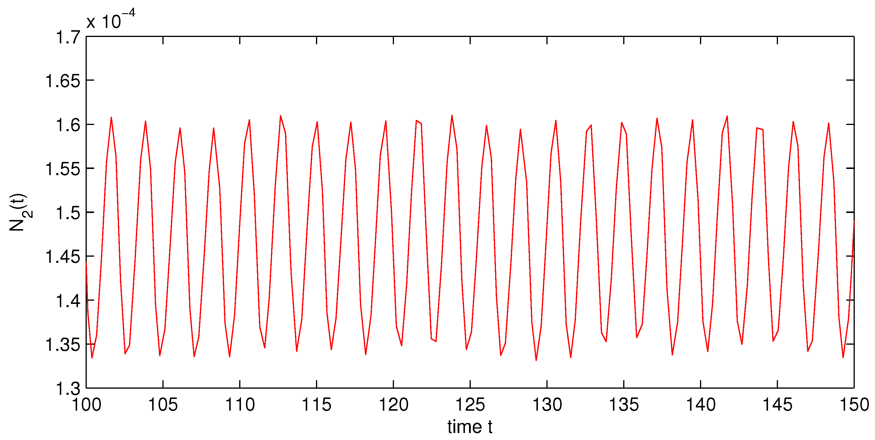
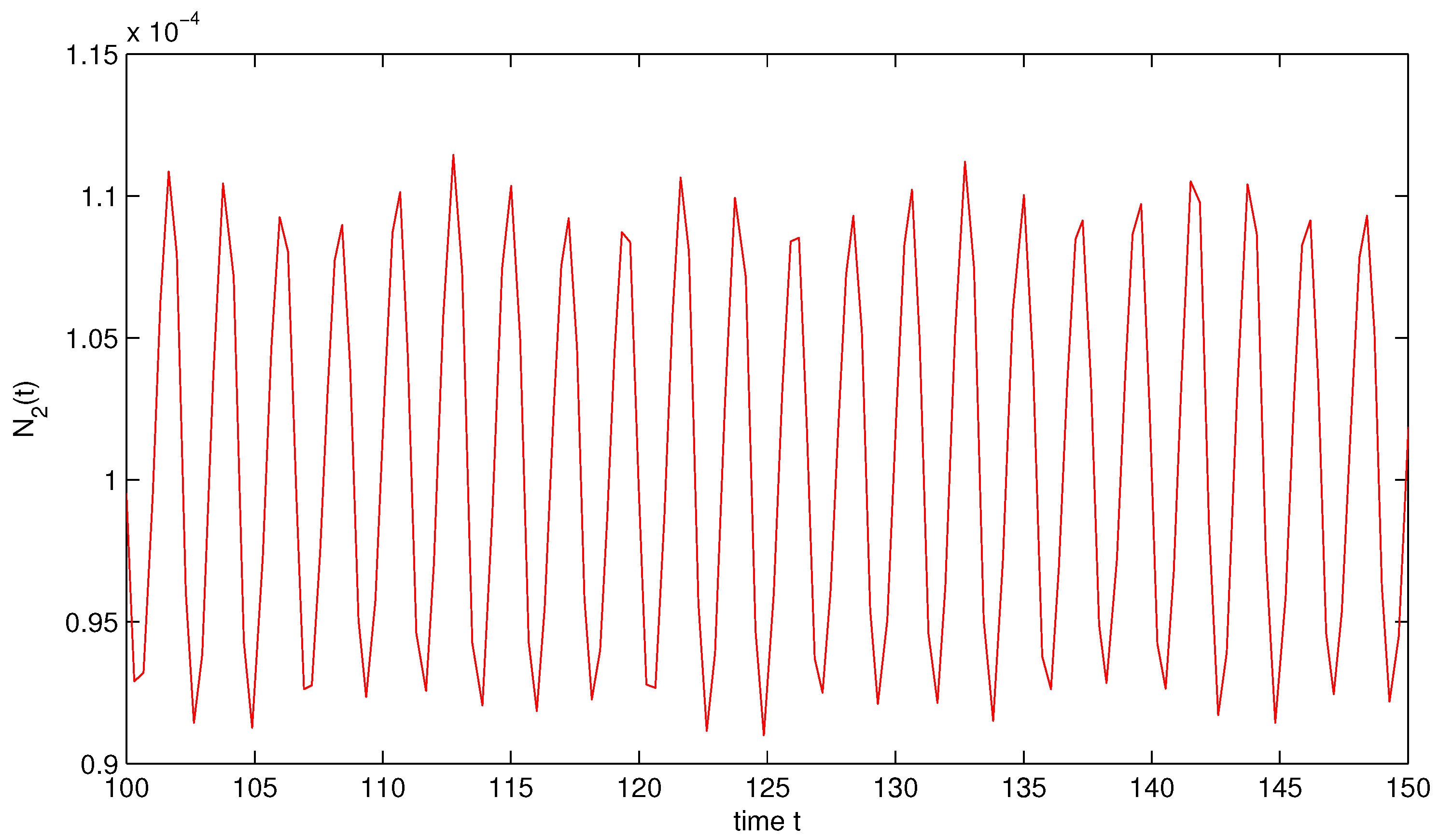
4. Two Examples and Numerical Simulations

Example 2. Consider the following delayed predator–prey model with Hassell-Varley type functional response:

$$\begin{array}{c}\hfill \left\{\begin{array}{c}{\dot{N}}_1\left(t\right)=N_1\left(t\right)\left[2-(10+{cos}^2\left(\sqrt{3}t\right))N_1\left(t\right)-\frac{e^{-17}{N}_2(t-1)}{10N_2^{0.5}(t-1)+N_1\left(t\right)}\right]\hfill \\ {\dot{N}}_2\left(t\right)=N_2\left(t\right)\left[-(1+0.1|sin\left(\sqrt{3}t\right)\left|\right)+\frac{(1+|sin\left(\sqrt{2}t\right)\left|\right)N_1(t-2)}{10N_2^{0.5}\left(t\right)+N_1(t-2)}\right]\hfill \end{array}\right.\end{array}$$

(31)

Then System (31) has at least one positive almost periodic solution.

Proof. Corresponding to System (4), we have $a=2$, $b\left(s\right)=10+{cos}^2\left(\sqrt{3}t\right)$, $c=e^{-17}$, $m=10$, $\theta =0.5$, $d=1+0.1|sin(\sqrt{3}t\left)\right|$ and $r\left(s\right)=1+|sin\left(\sqrt{2}t\right)|$, $\forall t\in \mathbb{R}$. Then $\overline{b}=10.5$ and $\overline{r}=1+\frac{2}{\pi }$. Choosing $\omega =4$ so that Equation (8) holds, that is, for $\forall t_0\in \mathbb{R}$,

$$\begin{array}{c}\hfill \frac{1}{T}{\int }_{t_0}^{t_0+T}a\left(s\right)\mathrm{d}s\in [1,3],\frac{1}{T}{\int }_{t_0}^{t_0+T}b\left(s\right)\mathrm{d}s\in [5.25,15.75],\forall T\ge 4.\end{array}$$

By an easy calculation, we obtain that

$${\rho }_1\approx 12,{\varrho }_1<34,\mu =2-0.1>1.9,$$

which implies that $\left(H_1\right)$ holds. By Theorem 1, System (31) gives at least one positive almost periodic solution (see Figure 1 and Figure 2). This completes the proof. ☐

Example 3. Consider the following delayed almost periodic predator–prey model with Hassell-Varley type functional response:

$$\begin{array}{c}\hfill \left\{\begin{array}{c}{\dot{N}}_1\left(t\right)=N_1\left(t\right)\left[2-\left(10+\frac{{cos}^2\left(\sqrt{2}t\right)+{cos}^2\left(\sqrt{3}t\right)}{2}\right)N_1\left(t\right)-\frac{e^{-17}{N}_2(t-1)}{10N_2^{0.5}(t-1)+N_1\left(t\right)}\right]\hfill \\ {\dot{N}}_2\left(t\right)=N_2\left(t\right)\left[-\left(1+\frac{|sin\sqrt{2}t|+|sin\sqrt{3}t|}{20}\right)+\frac{(1+|sin\left(\sqrt{2}t\right)\left|\right)N_1(t-2)}{10N_2^{0.5}\left(t\right)+N_1(t-2)}\right]\hfill \end{array}\right.\end{array}$$

(32)

In System (32), $|sin\sqrt{2}t|+|sin\sqrt{3}t|$ and ${cos}^2\left(\sqrt{2}t\right)+{cos}^2\left(\sqrt{3}t\right)$ are almost periodic functions, which are not periodic functions. Similar to the argument as given in Example 2, it is easy to prove that System (32) gives at least one positive almost periodic solution (see Figure 3 and Figure 4).

5. Conclusions

By using a fixed point theorem of coincidence degree theory, some criterions for the existence of positive almost periodic solution to a kind of delayed predator–prey model with Hassell-Varley type functional response are obtained. Theorem 1 provides sufficient conditions for the existence of a positive almost periodic solution to System (4). The results obtained in this paper are unprecedented, being different from the results obtained in [33,34]. Therefore, the method used in this paper provides a possible means to study the existence of positive almost periodic solutions to the models for biological populations.

References

1. Lotka, A.J. Elements of Physical Biology; Williams and Wilkins: Baltimore, MD, USA, 1925. [Google Scholar]
2. Volterra, V. Fluctuations in the abundance of species considered mathematically. Nature 1926, 118, 558–560. [Google Scholar] [CrossRef]
3. Ma, Z. Mathematical Modelling and Study of Species Ecology; Anhui Education Publishing Company: Hefei, China, 1996. [Google Scholar]
4. Chen, L.; Song, X.; Lu, Z. Mathematical Models and Methods in Ecology; Scientific and Technical Publisher of Sichuan: Chengdu, China, 2003. [Google Scholar]
5. Huo, H.F.; Li, W.T. Stable periodic solution of the discrete periodic Leslie-Gewer predator-prey model. Math. Comput. Model. 2004, 40, 261–269. [Google Scholar] [CrossRef]
6. Hsu, S.B.; Hwang, T.W.; Kuang, Y. Global analysis of the Michaelis-Menten type ratio-dependent predator-prey system. J. Math. Biol. 2001, 42, 489–506. [Google Scholar] [CrossRef] [PubMed]
7. Liu, S.; Beretta, E. A stage-structured predator-prey model of Beddington-DeAngelis type. SIAM J. Appl. Math. 2006, 66, 1101–1129. [Google Scholar] [CrossRef]
8. Fan, M.; Kuang, Y. Dynamics of a nonautonomous predator-prey system with the Beddington-DeAngelis functional. J. Math. Anal. Appl. 2004, 295, 15–39. [Google Scholar] [CrossRef]
9. Wang, H.; Zhong, S. Asymptotic behavior of solutions in nonautonomous predator-prey patchy system with beddington-type functional response. J. Appl. Math. Comput. 2006, 172, 122–140. [Google Scholar] [CrossRef]
10. Wang, H.L. Dispersal permanence of periodic predator-prey model with Ivlev-type functional response and impulsive effects. Appl. Math. Model. 2010, 34, 3713–3725. [Google Scholar] [CrossRef]
11. Ding, X.; Lu, C.; Liu, M. Periodic solutions for a semi-ratio-dependent predator-prey system with nonmonotonic functional response and time delay. Nonlinear Anal. RWA 2008, 9, 762–775. [Google Scholar] [CrossRef]
12. Wei, F.Y. Existence of multiple positive periodic solutions to a periodic predator-prey system with harvesting terms and Holling III type functional response. Commun. Nonlinear Sci. Numer. Simulat. 2011, 16, 2130–2138. [Google Scholar] [CrossRef]
13. Liu, G.R.; Yan, J.R. Positive periodic solutions for neutral delay ratio-dependent predator-prey model with Holling type III functional response. Appl. Math. Comput. 2011, 218, 4341–4348. [Google Scholar] [CrossRef]
14. Hassell, M.; Varley, G. New inductive population model for insect parasites and its bearing on biological control. Nature 1969, 223, 1133–1136. [Google Scholar] [CrossRef] [PubMed]
15. Cosner, C.; DeAngelis, D.; Ault, J.; Olson, D. Effects of spatial grouping on the functional response of predators. Theor. Popul. Biol. 1999, 56, 65–75. [Google Scholar] [CrossRef] [PubMed]
16. Hsu, S.B.; Hwang, T.W.; Kuang, Y. Global dynamics of a predator-prey model with Hassell-Varley type functional response. J. Math. Biol. 2008, 10, 1–15. [Google Scholar]
17. Wang, K. Periodic solutions to a delayed predator-prey model with Hassell-Varley type functional response. Nonlinear Anal. RWA 2011, 12, 137–145. [Google Scholar] [CrossRef]
18. Zhang, T.W. Multiplicity of positive almost periodic solutions in a delayed Hassell-Varleytype predator-prey model with harvesting on prey. Math. Meth. Appl. Sci. 2013, 37, 686–697. [Google Scholar]
19. Zhang, T.W.; Li, Y.K.; Ye, Y. Persistence and almost periodic solutions for a discrete fishing model with feedback control. Commun. Nonlinear Sci. Numer. Simul. 2011, 16, 1564–1573. [Google Scholar] [CrossRef]
20. Zhang, T.W.; Li, Y.K.; Ye, Y. On the existence and stability of a unique almost periodic solution of Schoener’s competition model with pure-delays and impulsive effects. Commun. Nonlinear Sci. Numer. Simul. 2012, 17, 1408–1422. [Google Scholar] [CrossRef]
21. Zhang, T.W.; Gan, X.R. Existence and permanence of almost periodic solutions for Leslie-Gower predator-prey model with variable delays. Elect. J. Differ. Equa. 2013, 2013, 1–21. [Google Scholar]
22. Zhang, T.W.; Gan, X.R. Almost periodic solutions for a discrete fishing model with feedback control and time delays. Commun. Nonlinear Sci. Numer. Simulat. 2014, 19, 150–163. [Google Scholar] [CrossRef]
23. Zhang, T.W. Almost periodic oscillations in a generalized Mackey-Glass model of respiratory dynamics with several delays. Int. J. Biomath. 2014, 7, 1450029. [Google Scholar] [CrossRef]
24. Shu, J.Y.; Zhang, T.W. Multiplicity of almost periodic oscillations in a harvesting mutualism model with time delays. Dynam. Cont. Disc. Impul. Syst. B Appl. Algor. 2013, 20, 463–483. [Google Scholar]
25. Liao, Y.Z.; Zhang, T.W. Almost periodic solutions of a discrete mutualism model with variable delays. Discret. Dyn. Nat. Soc. 2012, 2012, 742102. [Google Scholar] [CrossRef]
26. Zhang, T.W.; Li, Y.K. Positive periodic solutions for a generalized impulsive n-species Gilpin-Ayala competition system with continuously distributed delays on time scales. Int. J. Biomath. 2011, 4, 23–34. [Google Scholar] [CrossRef]
27. Fazly, M.; Hesaaraki, M. Periodic solutions for predator-prey systems with Beddington-DeAngelis functional response on time scales. Nonlinear Anal. RWA 2008, 9, 1224–1235. [Google Scholar] [CrossRef]
28. Zhu, Y.L.; Wang, K. Existence and global attractivity of positive periodic solutions for a predator-prey model with modified Leslie-Gower Holling-type II schemes. J. Math. Anal. Appl. 2011, 384, 400–408. [Google Scholar] [CrossRef]
29. Zhao, C.J. On a periodic predator-prey system with time delays. J. Math. Anal. Appl. 2007, 331, 978–985. [Google Scholar] [CrossRef]
30. Wang, K. Existence and global asymptotic stability of positive periodic solution for a predator-prey system with mutual interference. Nonlinear Anal. RWA 2009, 10, 2774–2783. [Google Scholar] [CrossRef]
31. Wang, K.; Zhu, Y.L. Global attractivity of positive periodic solution for a Volterra model. Appl. Math. Comput. 2008, 203, 493–501. [Google Scholar] [CrossRef]
32. Ding, X.Q.; Jiang, J.F. Periodicity in a generalized semi-ratio-dependent predator-prey system with time delays and impulses. J. Math. Anal. Appl. 2009, 360, 223–234. [Google Scholar] [CrossRef]
33. Liu, G.R.; Yan, J.R. Existence of positive periodic solutions for neutral delay Gause-type predator-prey system. Appl. Math. Model. 2011, 35, 5741–5750. [Google Scholar] [CrossRef]
34. Zhang, G.D.; Shen, Y.; Chen, B.S. Positive periodic solutions in a non-selective harvesting predator-prey model with multiple delays. J. Math. Anal. Appl. 2012, 395, 298–306. [Google Scholar] [CrossRef]
35. Fink, A.M. Almost Periodic Differential Equation; Spring-Verlag: Berlin, Germany; Heidleberg, Germany; New York, NY, USA, 1974. [Google Scholar]
36. He, C.Y. Almost Periodic Differential Equations; Higher Education Publishing House: Beijing, China, 1992. (In Chinese) [Google Scholar]
37. Gaines, R.; Mawhin, J. Coincidence Degree and Nonlinear Differential Equations; Springer Verlag: Berlin, Germany, 1977. [Google Scholar]
38. Zhang, G.D.; Shen, Y.; Chen, B.S. Bifurcation analysis in a discrete differential-algebraic predator-preysystem. Appl. Math. Model. 2014, 38, 4835–4848. [Google Scholar] [CrossRef]
39. Zhang, S.N.; Zheng, G. Almost periodic solutions of delay difference systems. Appl. Math. Comput. 2002, 131, 497–516. [Google Scholar] [CrossRef]
Figure 1. State variable N 1 of System (31).
Mca 21 00010 g001
Figure 2. State variable N 2 of System (31).
Mca 21 00010 g002
Figure 3. State variable N 1 of System (32).
Mca 21 00010 g003
Figure 4. State variable N 2 of System (32).
Mca 21 00010 g004