Holographic Tachyon in Fractal Geometry

Abstract

The search of a logical quantum gravity theory is one of the noteworthy issues in modern theoretical physics. It is known that most of the quantum gravity theories describe our universe as a dimensional flow. From this point of view, one can investigate whether and how these attractive properties are related with the ultraviolet-divergence problem. These important points motivated us to discuss the reconstruction of a scalar field problem in the fractal theory which is a well-known quantum theory of gravity. Making use of time-like fractal model and considering the holographic description of galactic dark energy, we implement a correspondence between the tachyon model of galactic dark energy effect and holographic energy. Such a connection gives us an opportunity to redefine the fractal dynamics of selected scalar field representation by considering the time-evolution of holographic energy.

1. Introduction

The recent galactic observations (type Ia supernovae (SNe-Ia) [1], Wilkinson Microwave Anisotropy Probe (WMAP) [2], Sloan Digital Sky Survey (SDS) [3], X-Ray [4], Planck-2013 [5]) give very important evidence that indicate that the universe appears to be expanding at an increasing rate. It is commonly accepted that this mysterious behavior comes from the existence of exotic dark components: 26.8 percent dark matter and 68.3 percent dark energy [5]. Other ordinary cosmic matters occupy the remaining 4.9 percent of the Universe. Investigating the dynamics of these exotic contents has been one of the leading research fields in astrophysics and cosmology.

In literature, the holographic dark energy model has attracted many scientists due to its interesting features such as describing a relationship between the cosmic horizon and galactic dark energy effect [6,7,8]. Recently, Campo et al. [9] have given a summary about different cases of the holographic prescription of dark energy with observational evidence. Additionally, plenty of theoretical investigations introduce the form of holographic energy density that are motivated from some physical principles including holography [10,11]. Scalar field models of galactic dark effect may be regarded as a suitable definition and naturally arise in String/M theory, particle physics, and super-symmetric version of field theories. Thus, the scalar field representations are expected to define the dynamical dark mechanism of our universe [12]. Like String/M theory, several fundamental theories give many scalar field definitions but cannot predict a formulation for the corresponding potential. A large number of scientists believe that time-varying definitions of the galactic dark energy effect give more meaningful conclusions than the cosmological constant [13]. The holographic energy density describes is a dynamical space-time model, that’s why it is natural to study the model in a dynamical framework such as fractal gravity instead of general relativity. For all we mentioned above, it is meaningful to investigate a scalar field in the framework of fractal theory. In light of the above studies, we are motivated to establish the dynamics of fractal tachyon by making use of the holographic energy description. Here, we mainly construct a connection between the holographic definition of the galactic dark energy effect and tachyon scalar field.

Our investigation is structured in four sections. The first one introduces the scope and purpose of the paper. The second one provides a summary of the fractal theory and some preliminaries. The third section of the work is a set of two different dark gravity scenarios: the non-interacting and interacting cases. The fourth section is devoted to concluding remarks.

2. Preliminaries

As a first step, we consider holographic energy associated with a flat Friedmann–Robertson–Walker type background that is compatible with the recent cosmological data [14,15]:

$$d{s}^2=A^2(t)\left[d{r}^2+r^2(d{\mathsf{\theta }}^2+{\sin }^2\mathsf{\theta }d{\mathsf{\phi }}^2)\right]-d{t}^2$$

(1)

where $A(t)$ denotes the cosmic scale factor which measures the cosmological expansion.

In fractal theory, the corresponding action is given as [16,17]

$$S=\frac{1}{2{\mathsf{\kappa }}^2}\int d\mathsf{\zeta }\sqrt{-g}[R-\mathsf{\eta }{\partial }_{\mathsf{\mu }}\mathsf{\upsilon }{\partial }^{\mathsf{\mu }}\mathsf{\upsilon }]+\int d\mathsf{\zeta }\sqrt{-g}{\pounds }_m$$

(2)

Here, ${\mathsf{\kappa }}^2=8\mathsf{\pi }G$ and $G$, $R$, $g$ and ${\pounds }_m$ describe the gravitational constant, Ricci curvature scalar, determinant of the metric tensor $g_{\mathsf{\mu }\mathsf{\nu }}$ and matter part of total lagrangian density, respectively. Additionally, $\mathsf{\upsilon }$ defines the fractal function while $\mathsf{\eta }$ is known as the fractal parameter. Note that $d\mathsf{\zeta }(x)$ shows the LebesgueStieltjes measurement that generalizes that $d^{4}x$ and $[\mathsf{\zeta }]=-D\mathsf{\alpha }$ is the dimension of $\mathsf{\zeta }$ where $\mathsf{\alpha }$ is a random positive constant. The fractal model of gravitation has three important properties: the theory is (i) Lorentz invariant; (ii) free from ultraviolet divergence; and (iii) power-counting renormalizable [18].

Calcagni [16,17] has recently studied the quantum theory of gravity in a fractal space-time to investigate cosmology in fractal geometry. Assuming a time-like fractal model in four-dimensions, i.e., $\mathsf{\upsilon }=t^{-\mathsf{\beta }}$ where $\mathsf{\beta }=4-4\mathsf{\alpha }$ shows the fractal dimension, Calcagni [17] found the following Friedmann-equation:

$$H^2=\frac{1}{3M_p^2}({\mathsf{\rho }}_h+{\mathsf{\rho }}_m+{\mathsf{\rho }}_f)$$

(3)

where ${\mathsf{\rho }}_f$ defines the fractal energy density which is given in the following form

$${\mathsf{\rho }}_f=3M_p^2\mathsf{\beta }\left(\frac{H}{t}-\frac{\mathsf{\eta }\mathsf{\beta }}{6t^{2(\mathsf{\beta }+1)}}\right)$$

(4)

Furthermore, ${\mathsf{\rho }}_m$ is the dark matter density while ${\mathsf{\rho }}_h$ shows the density of holographic energy inside the fractal universe, $M_p^{-2}=8\mathsf{\pi }G$ describes the reduced Planck mass, $H=\frac{1}{A}\frac{dA}{dt}$ shows the Hubble parameter and $\mathsf{\beta }=0$ gives the infrared sector, while $\mathsf{\beta }=2$ implies the ultraviolet era. One more thing, we further assume a pressureless dark matter condition, i.e., $p_m=0$.

Nonetheless, the fractal continuity equation is obtained as [16]:

$$\dot{\mathsf{\rho }}+(3H-\frac{\mathsf{\beta }}{t})(\mathsf{\rho }+p)=0$$

(5)

where $\mathsf{\rho }$ defines total dark energy density while $p$ shows total pressure.

On the other hand, the fractal gravitational constraint [17] is

$$\dot{H}+3H^2+\left(2+\frac{3\mathsf{\eta }}{t^{2\mathsf{\beta }}}\right)\frac{\mathsf{\beta }H}{t}-\frac{\mathsf{\beta }(\mathsf{\beta }+1)}{t^2}-\frac{\mathsf{\eta }\mathsf{\beta }(2\mathsf{\beta }+1)}{t^{2\mathsf{\beta }+2}}=0$$

(6)

The above relation can be transformed into another constraint given in General Relativity in the infrared regime. Next, in the ultraviolet era, the corresponding gravitational constraint becomes

$$\dot{H}+3H^2+\left(2+\frac{3\mathsf{\eta }}{t^4}\right)\frac{2H}{t}-\frac{6}{t^2}-\frac{10\mathsf{\eta }}{t^6}=0$$

(7)

Solving this equation yields [17]:

$$H(t)=-\frac{2}{t}-\frac{22\mathsf{\eta }}{13t^5}\frac{{}_1{F}_1(\frac{15}{4};\frac{17}{4};\frac{3\mathsf{\eta }}{2t^4})}{{}_1{F}_1(\frac{11}{4};\frac{13}{4};\frac{3\mathsf{\eta }}{2t^4})}$$

(8)

$$A^3(t)=t^{-6}\mathsf{\Theta }(\frac{11}{4};\frac{13}{4};\frac{3\mathsf{\eta }}{2t^4})$$

(9)

Here, ${}_1{F}_1$ is known as the first kind Kummer's confluent hypergeometric function and it is given as:

$${}_1{F}_1(a;b;x)\equiv \frac{\mathsf{\Gamma }(b)}{\mathsf{\Gamma }(a)}{\displaystyle \sum }_{n=0}^{+\infty }\frac{\mathsf{\Gamma }(a+n)}{\mathsf{\Gamma }(b+n)}\frac{x^n}{n!}$$

(10)

Introducing the following definitions of dimensionless density parameters

$${\mathsf{\Omega }}_h=\frac{{\mathsf{\rho }}_h}{3H^2{M}_p^2},{\mathsf{\Omega }}_m=\frac{{\mathsf{\rho }}_m}{3H^2{M}_p^2},{\mathsf{\Omega }}_f=\frac{{\mathsf{\rho }}_f}{3H^2{M}_p^2}$$

(11)

helps us to rewrite the fractal Friedmann equation in another very useful and simple form that can be written as:

$${\displaystyle \sum }_{i=h,m,f}{\mathsf{\Omega }}_i\equiv 1$$

(12)

where

$${\mathsf{\Omega }}_i\equiv ({\mathsf{\Omega }}_h,{\mathsf{\Omega }}_f,{\mathsf{\Omega }}_m)$$

(13)

Here, ${\mathsf{\Omega }}_f$ denotes the fractal density contribution. One last thing—the deceleration parameter is calculated as [18]:

$$q=-1-\frac{\dot{H}}{H^2}=-\frac{{\mathsf{\lambda }}_1}{{\mathsf{\lambda }}_2}$$

(14)

where

$$\begin{array}{ll}{\mathsf{\lambda }}_1=& 169(3t^4+\mathsf{\eta }){(t^4+2\mathsf{\eta })}_1{F}_1{(\frac{11}{4};\frac{13}{4};\frac{3\mathsf{\eta }}{2t^4})}^2\\ & +52\mathsf{\eta }{(2t^4+\mathsf{\eta })}_1{F}_1{(\frac{11}{4};\frac{13}{4};\frac{3\mathsf{\eta }}{2t^4})}_1{F}_1(\frac{11}{4};\frac{17}{4};\frac{3\mathsf{\eta }}{2t^4})\\ & -16{\mathsf{\eta }}^2{}_1{F}_1{(\frac{11}{4};\frac{17}{4};\frac{3\mathsf{\eta }}{2t^4})}^2\end{array}$$

(15)

$$\sqrt{\frac{{\mathsf{\lambda }}_2}{2}}=13t^4{}_1{F}_1(\frac{11}{4};\frac{13}{4};\frac{3\mathsf{\eta }}{2t^4})+11{\mathsf{\eta }}_1{F}_1(\frac{15}{4};\frac{17}{4};\frac{3\mathsf{\eta }}{2t^4})$$

(16)

It is seen that [18] the deceleration parameter behaves like $q\sim -1-\frac{5t^4}{2\mathsf{\eta }}$ for positive $\mathsf{\eta }$ and $q\sim -\frac{2}{5}$ for negative $\mathsf{\eta }$ values at the early times while $q\sim -\frac{3}{2}$ for both negative and positive $\mathsf{\eta }$ values at the late times.

3. Tachyonic Reconstruction of Holographic Energy

3.1. The Basic Scenario

The conservation equations in this scenario read:

$${\dot{\mathsf{\rho }}}_m+\left(3H-\frac{\mathsf{\beta }}{t}\right){\mathsf{\rho }}_m=0$$

(17)

$${\dot{\mathsf{\rho }}}_h+\left(3H-\frac{\mathsf{\beta }}{t}\right)(1+{\mathsf{\omega }}_h){\mathsf{\rho }}_h=0$$

(18)

Note that we have defined that ${\mathsf{\omega }}_h=\frac{p_h}{{\mathsf{\rho }}_h}$ in the above relations.

The well-known holographic dark energy density has the following form:

$${\mathsf{\rho }}_h=3c^2{M}_p^2{H}^2$$

(19)

where $c^2$ is a random constant, and the Hubble radius is chosen as $L=\frac{1}{H}$ as the infrared cut-off of the system [11]. It is significant to talk about here that, in general, the value of $c^2$ can change in time very slowly, which means that the Hubble expansion rate bounds $\frac{1}{c^2}\frac{d{c}^2}{dt}$ [18,19]:

$$\frac{1}{c^2}\frac{d{c}^2}{dt}\le H$$

(20)

It worth emphasizing here that the above case must be satisfied throughout the history of the Universe; otherwise, the density of dark energy cannot be proportional to $\frac{1}{L^2}$ at the core of holography [11,19]. Radicella and Pavon [19] showed that $c^2$ is the infrared length dependent and can be taken as constant in the late time era where the galactic dark contents dominate the Universe. Therefore, inserting relation Equation (18) in Equation (3) gives:

$${\mathsf{\xi }}_1+{\mathsf{\xi }}_2=\frac{1-c^2}{c^2}$$

(21)

where ${\mathsf{\xi }}_1=\frac{{\mathsf{\rho }}_m}{{\mathsf{\rho }}_h}$ and ${\mathsf{\xi }}_2=\frac{{\mathsf{\rho }}_f}{{\mathsf{\rho }}_h}$ are the energy density ratios. From this result, we see that the aggregate energy density ratio will be a constant and the coincidence problem may be eased. Time derivatives of both sides of Equation (19) with the help of fractal Friedmann Equation (3) yields:

$${\dot{\mathsf{\rho }}}_h=\frac{3c^2{M}_p^2}{\frac{\mathsf{\beta }}{2Ht}-1}\left[{\mathsf{\Omega }}_h{H}^2(3H-\frac{\mathsf{\beta }}{t})(\frac{1}{c^2}+{\mathsf{\omega }}_h)+\mathsf{\beta }\mathsf{\mu }\right]$$

(22)

where

$$\mathsf{\mu }=\frac{3H^2}{t}-\frac{H}{t^2}(\mathsf{\beta }-1)-\frac{\mathsf{\eta }\mathsf{\beta }H}{2t^{2\mathsf{\beta }+2}}-\frac{\mathsf{\eta }\mathsf{\beta }(\mathsf{\beta }+2)}{6t^{2\mathsf{\beta }+3}}$$

(23)

Therefore, inserting this result into the fractal continuity relation Equation (18) and considering the dimensionless density parameters defined in the second section, we find:

$${\mathsf{\omega }}_h=-1+\frac{1-c^2+\frac{\mathsf{\beta }\mathsf{\mu }}{{\mathsf{\Omega }}_h{H}^2{c}^2}{(3H-\frac{\mathsf{\beta }}{t})}^{-1}}{1-c^2-\frac{\mathsf{\beta }}{2Ht}}$$

(24)

In the absence of fractal contributions, i.e., $\mathsf{\beta }=0$, we encounter the dust case with ${\mathsf{\omega }}_h=0$. Next, for the $\mathsf{\beta }=2$ value, we can use Equations (7) and (9) to obtain the exact form of equation-of-state parameter ${\mathsf{\omega }}_h$. Hence, we get

$$\underset{\mathsf{\beta }\to 2}{\lim }{\mathsf{\omega }}_h=-1+\frac{1-c^2+\frac{2\tilde{\mathsf{\mu }}}{{\mathsf{\Omega }}_h{H}^2{c}^2}{(3H-\frac{2}{t})}^{-1}}{1-c^2-\frac{1}{Ht}}$$

(25)

where

$$\tilde{\mathsf{\mu }}=\frac{3H^2}{t}-\frac{H}{t^2}-\frac{\mathsf{\eta }H}{t^6}-\frac{4\mathsf{\eta }}{3t^7}$$

(26)

$$H(t)=-\frac{2}{t}-\frac{22\mathsf{\eta }}{13t^5}\frac{\mathsf{\Gamma }(\frac{17}{4})\mathsf{\Gamma }(\frac{11}{4}){\sum }_{n=0}^{+\infty }\frac{\mathsf{\Gamma }(\frac{15}{4}+n)}{\mathsf{\Gamma }(\frac{17}{4}+n)}\frac{{\left(\frac{3\mathsf{\eta }}{2t^4}\right)}^n}{n!}}{\mathsf{\Gamma }(\frac{15}{4})\mathsf{\Gamma }(\frac{13}{4}){\sum }_{m=0}^{+\infty }\frac{\mathsf{\Gamma }(\frac{11}{4}+m)}{\mathsf{\Gamma }(\frac{13}{4}+m)}\frac{{\left(\frac{3\mathsf{\eta }}{2t^4}\right)}^m}{m!}}$$

(27)

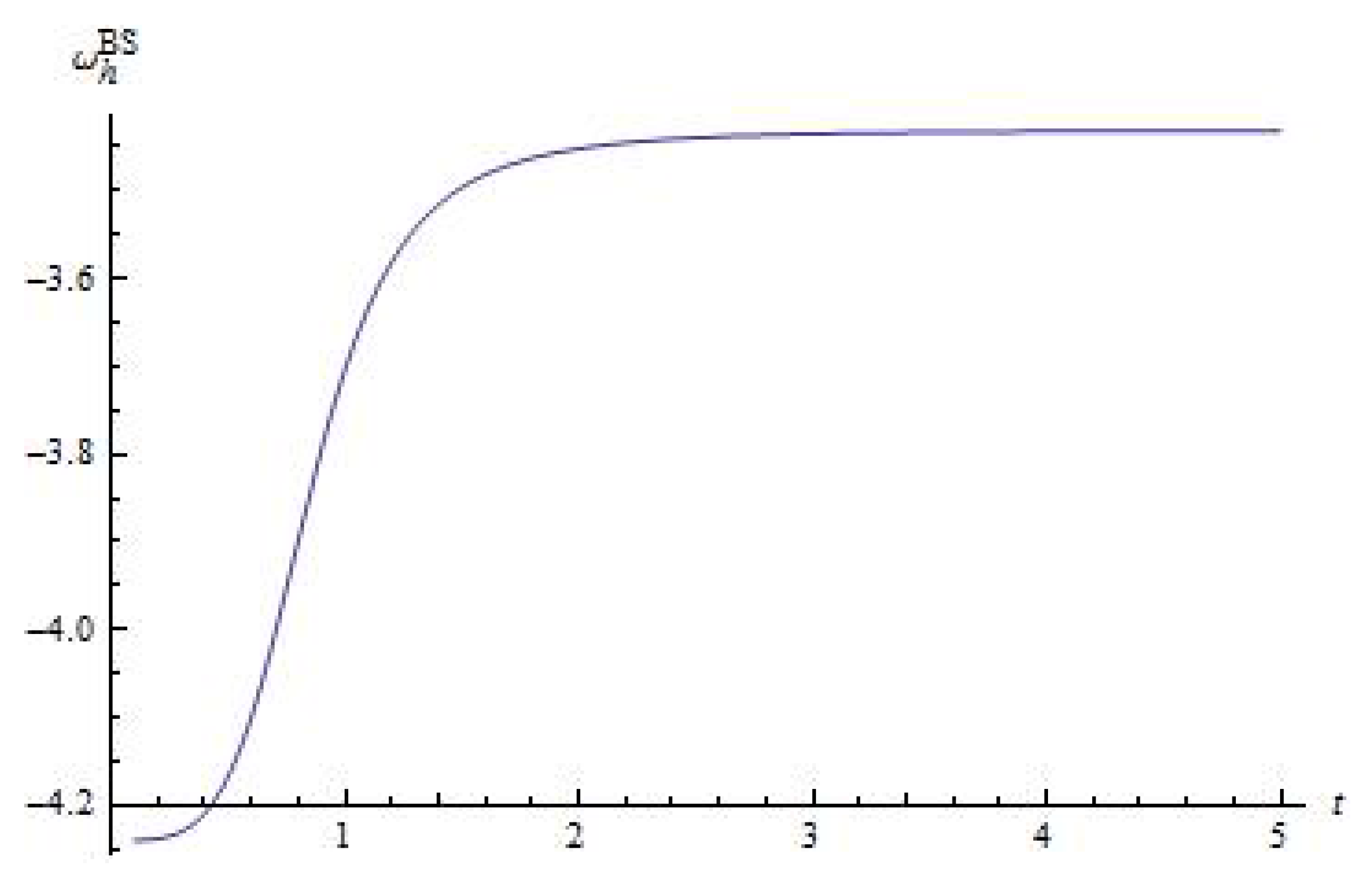
In Figure 1, we analyzed numerically [20] the time evolution of the equation-of-state parameter of the holographic model introduced for the galactic dark energy effect in fractal geometry. From this figure we see that ${\omega }_h{}^{BS}$ have values smaller than -1 (it is easy to see that ${\omega }_h{}^{BS}<-1$ especially at early times) which means the equation-of-state parameter in basic scenario may cross the phantom divide, i.e. ${\omega }_h=-1$, at all times.

At this step, we are in a position to construct the connection between the holographic dark energy and tachyonic field. As we have mentioned in the first section, the tachyon scalar field had been proposed as one of the possible dark energy candidates. This dark energy candidate has an interesting nature of the equation-of-state parameter, and the quantity takes values between $-1$ and $0$ [13,21]. From this point of view, the tachyon field is considered as a source of dark energy as well as one of the possible candidates explaining the inflation at high energy [22,23]. The effective Lagrangian density of the tachyonic field is defined as:

$${\pounds }_T=V(\mathsf{\phi })\sqrt{1-g^{\mathsf{\mu }\mathsf{\nu }}{\partial }_{\mathsf{\mu }}\mathsf{\phi }{\partial }_{\mathsf{\nu }}\mathsf{\phi }}$$

(28)

where $V(\mathsf{\phi })$ is a tachyonic potential and $g^{\mathsf{\mu }\mathsf{\nu }}$ represents the inverse metric. For the tachyon field, the energy and pressure densities are defined, respectively, as [24]:

$${\mathsf{\rho }}_T=V(\mathsf{\phi }){(1-{\dot{\mathsf{\phi }}}^2)}^{-1/2},p_T=-V(\mathsf{\phi }){(1-{\dot{\mathsf{\phi }}}^2)}^{1/2}$$

(29)

Thus, we have ${\mathsf{\omega }}_T={\dot{\mathsf{\phi }}}^2-1$. Note that $-1<\dot{\mathsf{\phi }}<1$ is the required condition to describe a real tachyonic energy density [25]. Nonetheless, $-1<{\mathsf{\omega }}_T<0$ is the corresponding constraint for the equation-of-state parameter of tachyon. The tachyon scalar field can describe a universe with accelerated expansion, but it cannot behave like phantom energy [13]. Comparing Equations (18) and (27), we get the following expression of the tachyon potential:

$$V(\mathsf{\phi })={\mathsf{\rho }}_h{(1-{\dot{\mathsf{\phi }}}^2)}^{1/2}$$

(30)

and, by making use of Equations (22) and the definition of ${\mathsf{\omega }}_T$, we can write:

$${\dot{\mathsf{\phi }}}^2=1+{\mathsf{\omega }}_h=\frac{1-c^2+\frac{\mathsf{\beta }\mathsf{\mu }}{{\mathsf{\Omega }}_h{H}^2{c}^2}{(3H-\frac{\mathsf{\beta }}{t})}^{-1}}{1-c^2-\frac{\mathsf{\beta }}{2Ht}}$$

(31)

Furthermore, using Equations (10), (30) and (31), the potential of tachyon can be rewritten as

$$V(\mathsf{\phi })={\mathsf{\rho }}_h{(-{\mathsf{\omega }}_h)}^{1/2}=3c^2{M}_p^2{H}^2\sqrt{1-\frac{1-c^2+\frac{\mathsf{\beta }\mathsf{\mu }}{{\mathsf{\Omega }}_h{H}^2{c}^2}{(3H-\frac{\mathsf{\beta }}{t})}^{-1}}{1-c^2-\frac{\mathsf{\beta }}{2Ht}}}$$

(32)

The relations of kinetic term ${\dot{\mathsf{\phi }}}^2$ and tachyonic potential $V(\mathsf{\phi })$ imply that these quantities may exist if it is provided that $-1\le {\mathsf{\omega }}_h\le 0$. This condition shows that the phantom energy sector cannot be crossed in a universe with an accelerated expansion.

Next, by using Equation (31), the evolutionary form of tachyon scalar field can easily be found:

$$\mathsf{\phi }(t)-\mathsf{\phi }(t_0)={\int }_{t_0}^t\sqrt{\frac{1-c^2+\frac{\mathsf{\beta }\mathsf{\mu }}{{\mathsf{\Omega }}_h{H}^2{c}^2}{(3H-\frac{\mathsf{\beta }}{t})}^{-1}}{1-c^2-\frac{\mathsf{\beta }}{2Ht}}}dt$$

(33)

The description of potential in terms of holographic fractal scalar field cannot be determined analytically due to the complexity of corresponding relations. From this point of view, it can be discussed numerically. In the absence of fractal contributions, Equation (33) yields $\mathsf{\phi }(t)=t$ (here, we set a vanishing integration constant).

3.2. The Interacting Scenario

In this part of our investigation, we extend our conclusions to the interacting scenario. Thus, the conservation equations in the presence of interaction yield:

$${\dot{\mathsf{\rho }}}_m+\left(3H-\frac{\mathsf{\beta }}{t}\right){\mathsf{\rho }}_m=\Sigma$$

(34)

$${\dot{\mathsf{\rho }}}_h+\left(3H-\frac{\mathsf{\beta }}{t}\right)(1+{\tilde{\mathsf{\omega }}}_h){\mathsf{\rho }}_h=-\Sigma$$

(35)

Here, we defined $\Sigma$ to describe the mutual interaction between two dominant exotic components of our Universe. Positive values of this parameter define the energy flow from the dark energy era to the dark matter divide, and the vice versa case occurs for the netative values of $\Sigma$ [26,27,28,29,30]. Recently, it has been reported that the Abell Cluster A586 observed a transition from the dark energy sector to the dark matter era and vice versa [31,32]. Next, this interesting case effectively occurs as a self-conserved exotic dark content [33,34,35]. Nonetheless, the significance of this interesting event has not been explained clearly [36]. For the interaction term, the first and natural assumption may be the Hubble factor, but it can also be in other meaningful forms: $\Sigma \propto H{\mathsf{\rho }}_h$, $\Sigma \propto H{\mathsf{\rho }}_m$ or $\Sigma \propto H({\mathsf{\rho }}_h+{\mathsf{\rho }}_m)$ [12]. We see that for all three forms of the interaction term, the equation of state parameter of fractal holographic dark energy has a similar form; therefore, hereafter, we assume that:

$$\Sigma =3{\mathsf{\gamma }}^{2}H{\mathsf{\rho }}_h$$

(36)

where $\mathsf{\gamma }$ is the coupling parameter for the dark components [37,38]. The sign of ${\mathsf{\gamma }}^2$ implies the direction of energy transition. The $\mathsf{\gamma }=0$ case denotes the non-interacting fractal Friedmann–Robertson–Walker type background, while $\mathsf{\gamma }=1$ shows the complete energy transfer from the dark energy divide to the dark matter region. In some particular cases, ${\mathsf{\gamma }}^2$ is assumed to be in the range of $[0,1]$ [39]. Furthermore, Cosmic Microwave Background and Galactic Clusters data indicate that ${\mathsf{\gamma }}^2<0.025$, i.e., a small but positive parameter of the order of unity [40,41].

Inserting Equations (20) and (36) in Equation (34), we find

$${\tilde{\mathsf{\omega }}}_h=-1+\frac{c^2-1-(\frac{\mathsf{\beta }}{2Ht}-1){(3H-\frac{\mathsf{\beta }}{t})}^{-1}\left[3{\mathsf{\gamma }}^{2}H+\frac{\mathsf{\beta }\mathsf{\mu }{c}^2}{H^2{\mathsf{\Omega }}_h}{(\frac{\mathsf{\beta }}{2Ht}-1)}^{-1}\right]}{c^2+\frac{\mathsf{\beta }}{2Ht}-1}$$

(37)

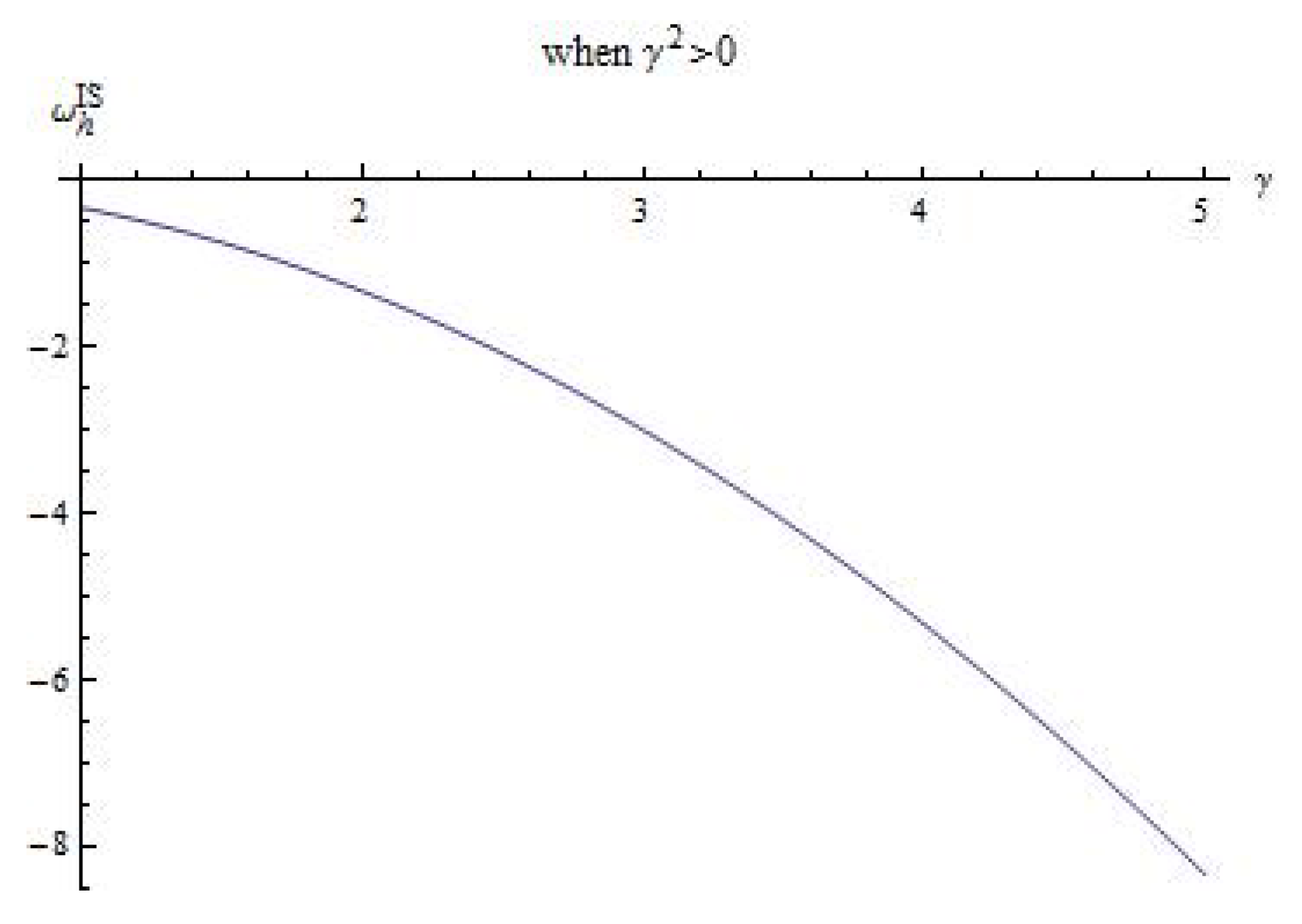
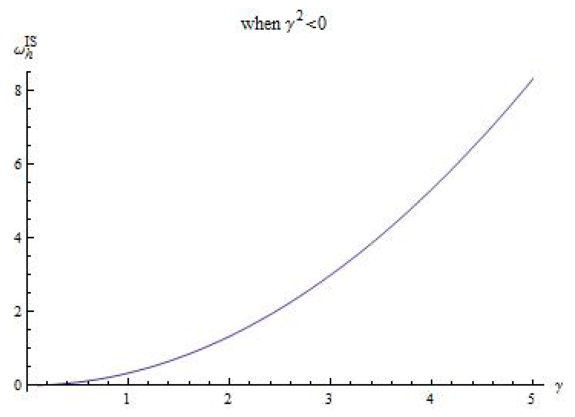
Without fractal contributions, i.e., $\mathsf{\beta }=0$, we have ${\tilde{\mathsf{\omega }}}_h=\frac{{\mathsf{\gamma }}^2}{c^2-1}$, which is the same as obtained in general relativity by Sheykhi in Ref. [12]. Furthermore, in the absence of interaction, i.e., ${\mathsf{\gamma }}^2=0$, we obtain the same conclusion given in the previous subsection. It is worth emphasizing here that, in order to have ${\tilde{\mathsf{\omega }}}_h<0$, we should have $c^2<1$. On the other hand, the accelerated galactic expansion may be defined if it is given that $c^2>1-3{\mathsf{\gamma }}^2$ (the condition gives ${\tilde{\mathsf{\omega }}}_h<\frac{1}{3}$); therefore, this model can explain the accelerated expansion if $1-3{\mathsf{\gamma }}^2<c^2<1$ and the holographic equation-of-state parameter can cross the phantom divide, i.e., ${\tilde{\mathsf{\omega }}}_h<-1$, when ${\mathsf{\gamma }}^2>1-c^2$ [12]. Figure 2 shows that the phantom region crossing can be achieved provided ${\mathsf{\gamma }}^2>0$, which is consistent with recent observational evidence [42,43]. At the same time, Figure 3 implies that ${\mathsf{\gamma }}^2<0$ leads to ${\tilde{\mathsf{\omega }}}_h>-\frac{1}{3}$, which means that the Universe is in deceleration phase, which is ruled out by recent data.

A connection between the tachyon scalar field and interacting fractal holographic dark energy can be constructed now. In further steps, it will be assumed that ${\mathsf{\gamma }}^2>0$. Thus, in this scenario, the time-evolution of fractal scalar field and its potential are calculated as:

$$\mathsf{\phi }(t)=\mathsf{\phi }(t_0)+{\int }_{t_0}^t\sqrt{\frac{c^2-1-(\frac{\mathsf{\beta }}{2Ht}-1){(3H-\frac{\mathsf{\beta }}{t})}^{-1}\left[3{\mathsf{\gamma }}^{2}H+\frac{\mathsf{\beta }\mathsf{\mu }{c}^2}{H^2{\mathsf{\Omega }}_h}{(\frac{\mathsf{\beta }}{2Ht}-1)}^{-1}\right]}{c^2+\frac{\mathsf{\beta }}{2Ht}-1}}dt$$

(38)

$$V(\mathsf{\phi })=3c^2{M}_p^2{H}^2\sqrt{\frac{1-c^2+(\frac{\mathsf{\beta }}{2Ht}-1){(3H-\frac{\mathsf{\beta }}{t})}^{-1}\left[3{\mathsf{\gamma }}^{2}H+\frac{\mathsf{\beta }\mathsf{\mu }{c}^2}{H^2{\mathsf{\Omega }}_h}{(\frac{\mathsf{\beta }}{2Ht}-1)}^{-1}\right]}{c^2+\frac{\mathsf{\beta }}{2Ht}-1}}$$

(39)

Using Equation (38) with the absence of the fractal contribution gives

$$\mathsf{\phi }(t)=t\sqrt{1+\frac{{\mathsf{\gamma }}^2}{c^2-1}}$$

(40)

Note that here we set the integration constant equal to zero. Combining Equation (27) with (39), the potential of tachyon scalar field is found as:

$$V(\mathsf{\phi })=\frac{3\mathsf{\gamma }{c}^2{M}_p^2{H}^2}{1-c^2}$$

(41)

These limiting results are exactly the same as obtained in Ref. [12] using the general theory of relativity. By making use of Equations (3) and (36) without fractal contributions, one can find

$$\frac{\dot{H}}{H^2}=\frac{3}{2}\left(\frac{{\mathsf{\gamma }}^2{c}^2}{1-c^2}-1\right)$$

(42)

and the first integration gives

$$H=\frac{\dot{A}}{A}=\frac{2}{3kt}$$

(43)

where $k=1+\frac{{\mathsf{\gamma }}^2{c}^2}{c^2-1}$ [12]. Now, considering Equations (39) and (42), one can write the potential of tachyon in terms of scalar field in the form:

$$V(\mathsf{\phi })=\frac{4\mathsf{\gamma }{c}^2{M}_p^2(1-c^2-{\mathsf{\gamma }}^2)}{3k^2{(1-c^2)}^{\frac{3}{2}}}\frac{1}{{\mathsf{\phi }}^2}$$

(44)

which corresponds to another inverse square power-law potential defined in the scaling solutions case [44,45,46].

4. Conclusions

Making use of the fractal form of holographic dark energy description and the tachyon scalar field set as the effective definition for the galactic dark energy effect, it is attractive to investigate how the holographic dark energy density can be used to define the fractal tachyon. Taking the fractal geometry into account, we have implemented a connection between the tachyon model of galactic dark energy and the holographic dark scenario. Assuming the fractal description of tachyon field as an effective theory of holographic energy, the selected scalar field should be allowed to mimic the evolving nature of dynamical holographic energy and re-implement the definition of scalar field using that evolutionary feature. Hence, with the help of this strategy, we have obtained a useful definition for the potential of holographic fractal tachyon and reconstructed the dynamics of fractal scalar field making use of the evolution of holographic energy density. We have also compared our results with those ones obtained in literature previously in the limiting cases.

Furthermore, we want to emphasize here that the presented results can be extended easily to other well-known scalar fields assumptions such as the dilaton, phantom, quintessence, kinetic quintessence (k-essence), chaplygin gas and polytropic gas. One can also generalize the aforementioned conclusions given in this study to the non-flat version of fractal Friedmann-Robertson-Walker space-time. Next, one can also write our results in terms of not the cosmic time t but the redshift parameter $z=\frac{A_{now}}{A_{then}}-1$ which implies an expanding Big Bang universe. In an expanding universe such as the one we have experienced, the scale factor increases monotonically as time passes, hence the redshift parameter has positive values which mean distant galaxies appear redshifted. On the other hand, (i) one can also extend our results by considering fractal description of the extended holographic energy [47], modified holographic Ricci dark energy [48], and new agegraphic dark energy [18], (ii) in Reference [49], the fractal ghost reconstruction of quintessence field was achieved. After comparing our manuscript with this paper, it can be seen that all of our results are agree with and extend those ones obtained in Reference [49].

References

- Perlmutter, S.; Aldering, G.; Goldhaber, G.; Knop, R.A.; Nugent, P.; Castro, P.G.; Deustua, S.; Fabbro, S.; Goobar, A.; Groom, D.E.; et al. Measurements of Ω and Λ from 42 High-Redshift Supernovae. Astrophys. J. 1999, 517, 2. [Google Scholar] [CrossRef]
- Bennet, C.L.; Halpern, M.; Hinshaw, G.; Jarosik, N.; Kogut, A.; Limon, M.; Meyer, S.S.; Page, L.; Spergel, D.N.; Tucker, G.S.; et al. First Year Wilkinson Microwave Anisotropy Probe (WMAP) Observations: Preliminary Maps and Basic Results. Astrophys. J. Suppl. 2003, 148, 1. [Google Scholar] [CrossRef]
- Tegmark, M.; Strauss, M.; Blanton, M.; Abazajian, K.; Dodelson, S.; Sandvik, H.; Wang, X.; Weinberg, D.; Zehavi, I.; Bahcall, N.; et al. Cosmological parameters from SDSS and WMAP. Phys. Rev. D 2004, 69, 103501. [Google Scholar] [CrossRef]
- Allen, A.W.; Schmidt, R.W.; Ebeling, H.; Fabian, A.C.; van Speybroeck, L. Constraints on dark energy from Chandra observations of the largest relaxed galaxy clusters. Mon. Not. Roy. Astron. Soc. 2004, 353, 457. [Google Scholar] [CrossRef]
- Ade, P.A.R.; Aghanim, N.; Armitage-Caplan, C.; Arnaud, M.; Ashdown, M.; Atrio-Barandela, F.; Aumont, J.; Baccigalupi, C.; Banday, A.J.; Barreiro, R.B.; et al. Planck 2013 results. XVI. Cosmological parameters. Astron. Astrophys. 2014, 571, A16. [Google Scholar]
- Ng, Y.J. From Computation to Black Holes and Space-Time Foam. Phys. Rev. Lett. 2001, 86, 2946. [Google Scholar] [CrossRef] [PubMed]
- Arzano, M.; Kephart, T.W.; Ng, Y.J. From spacetime foam to holographic foam cosmology. Phys. Lett. B 2007, 649, 243. [Google Scholar] [CrossRef]
- Duran, I.; Pavon, D. Holographic dark energy at the Ricci scale. J. Phys. Conf. Ser. 2011, 314, 012058. [Google Scholar] [CrossRef]
- del Campo, S.; Fabris, J.C.; Herrera, R.; Zimdahl, W. Holographic dark-energy models. Phys. Rev. D 2011, 83, 123006. [Google Scholar] [CrossRef]
- Sheykhi, A. Holographic scalar field models of dark energy. Phys. Rev. D 2011, 84, 107302. [Google Scholar] [CrossRef]
- Li, M.; Li, X.D.; Wang, S.; Wang, Y. Dark Energy. Commun. Theor. Phys. 2011, 56, 525. [Google Scholar] [CrossRef]
- Sheykhi, A.; Bagheri, A. Quintessence Ghost Dark Energy Model. Europhys. Lett. 2011, 95, 39001. [Google Scholar] [CrossRef]
- Pasqua, A.; Khodam-Mohammadi, A.; Jamil, M.; Myrzakulov, R. Interacting Ricci Dark Energy with Logarithmic Correction. Astrophys. Space Sci. 2012, 340, 199. [Google Scholar] [CrossRef]
- Komatsu, E.; Smith, K.M.; Dunkley, J.; Bennett, C.L.; Gold, B.; Hinshaw, G.; Jarosik, N.; Larson, D.; Nolta, M.R.; Page, L.; et al. Seven-year Wilkinson microwave anisotropy probe (wmap) observations: cosmological interpretation. Astrophys. J. Suppl. 2011, 192, 18. [Google Scholar] [CrossRef]
- Hinshaw, G.; Larson, D.; Komatsu, E.; Spergel, D.N.; Bennett, C.L.; Dunkley, J.; Nolta, M.R.; Halpern, M.; Hill, R.S.; Odegard, N.; et al. Nine-Year Wilkinson Microwave Anisotropy Probe (WMAP) Observations: Cosmological Parameter Results. Astrophys. J. Suppl. 2013, 208, 19. [Google Scholar] [CrossRef]
- Calcagni, G. Fractal Universe and Quantum Gravity. Phys. Rev. Lett. 2010, 104, 251301. [Google Scholar] [CrossRef] [PubMed]
- Calcagni, G. Quantum field theory, gravity and cosmology in a fractal universe. JHEP 2010, 03, 120. [Google Scholar] [CrossRef]
- Karami, K.; Jamil, M.; Ghaffari, S.; Fahimi, K. Holographic, new agegraphic and ghost dark energy models in fractal cosmology. Can. J. Phys. 2013, 91, 770. [Google Scholar] [CrossRef]
- Radicella, N.; Pavon, D. On the c2 term in the holographic formula for dark energy. JCAP 2010, 1010:005. [Google Scholar]
- Wolfram Research. Wolfram Mathematica 8.0; Wolfram Research Inc.: Long Hanborough Oxfordshire OX29 8FD, UK, 2010. [Google Scholar]
- Gibbons, G.W. Cosmological evolution of the rolling tachyon. Phys. Lett. B 2002, 537, 1. [Google Scholar] [CrossRef]
- Mazumdar, A.; Panda, S.; Perez-Lorenzana, A. Assisted inflation via tachyon condensation. Nucl. Phys. B 2001, 614, 101. [Google Scholar] [CrossRef]
- Padmanabhan, T. Accelerated expansion of the universe driven by tachyonic matter. Phys. Rev. D 2002, 66, 021301. [Google Scholar] [CrossRef]
- Jamil, M.; Karami, K.; Sheykhi, A. Restoring New Agegraphic Dark Energy in RS II Braneworld. Int. J. Theor. Phys. 2011, 50, 3069. [Google Scholar] [CrossRef]
- Sheykhi, A.; Movahed, M.S.; Ebrahimi, E. Tachyon Reconstruction of Ghost Dark Energy. Astrophys. Space Sci. 2012, 339, 93. [Google Scholar] [CrossRef]
- Jamil, M.; Saridakis, E.N.; Setare, M.R. Thermodynamics of dark energy interacting with dark matter and radiation. Phys. Rev. D 2010, 81, 023007. [Google Scholar] [CrossRef]
- Wetterich, C. The cosmon model for an asymptotically vanishing time-dependent cosmological constant. Astron. Astrophys. 1995, 301, 321. [Google Scholar]
- Amendola, L. Scaling solutions in general nonminimal coupling theories. Phys. Rev. D 1999, 60, 043501. [Google Scholar] [CrossRef]
- Zhang, X. Coupled Quintessence in a Power-Law Case and The Cosmic Coincidence Problem. Mod. Phys. Lett. A 2005, 20, 2575. [Google Scholar] [CrossRef]
- Gonzalez, T.; Leon, G.; Quiros, I. Dynamics of quintessence models of dark energy with exponential coupling to dark matter. Class. Quant. Grav. 2006, 23, 3165. [Google Scholar] [CrossRef]
- Bertolami, O.; Gil Pedro, F.; Le Delliou, M. Dark energy–dark matter interaction and putative violation of the equivalence principle from the Abell cluster A586. Phys. Lett. B 2007, 654, 165. [Google Scholar] [CrossRef]
- Jamil, M.; Rashid, M.A. Constraints on Coupling Constant Between Chaplygin Gas and Dark Matter. Eur. Phys. J. C 2008, 58, 111. [Google Scholar] [CrossRef]
- Sola, J.; Stefancic, H. Effective equation of state for dark energy: Mimicking quintessence and phantom energy through a variable Λ. Phys. Lett. B 2005, 624, 147. [Google Scholar] [CrossRef]
- Shapiro, I.L.; Sola, J. On the possible running of the cosmological constant. Phys. Lett. B 2009, 682, 105. [Google Scholar] [CrossRef]
- Grande, J.; Sola, J.; Stefancic, H. LXCDM: A Cosmon model solution to the cosmological coincidence problem? JCAP 2006, 011, 0608. [Google Scholar]
- Feng, C.; Wang, B.; Gong, Y.; Su, R.-K. Testing the viability of the interacting holographic dark energy model by using combined observational constraints. J. Cosmol. Astropart. Phys. 2007, 9, 5. [Google Scholar] [CrossRef]
- Amendola, L.; Tocchini-Valetini, D. Stationary dark energy: The present universe as a global attractor. Phys. Rev. D 2001, 64, 043509. [Google Scholar] [CrossRef]
- Setare, M.R.; Jamil, M. Correspondence between entropy-corrected holographic and Gauss-Bonnet dark-energy models. Phys. Lett. B 2010, 690, 1. [Google Scholar] [CrossRef]
- Zhang, H.; Zhu, Z.H. Interacting Chaplygin gas. Phys. Rev. D 2006, 73, 043518. [Google Scholar] [CrossRef]
- Ichiki, K.; Keum, Y.Y. Primordial Neutrinos, Cosmological Perturbations in Interacting Dark-Energy Model: CMB and LSS. J. Cosmol. Astropart. Phys. 2008, 6, 5. [Google Scholar] [CrossRef]
- Amendola, L.; Campos, G.C.; Rosenfeld, R. Consequences of dark matter-dark energy interaction on cosmological parameters derived from type Ia supernova data. Phys. Rev. D 2007, 75, 083506. [Google Scholar] [CrossRef]
- Wang, B.; Gong, Y.; Abdalla, E. Transition of the dark energy equation of state in an interacting holographic dark energy model. Phys. Lett. B 2005, 624, 141. [Google Scholar] [CrossRef]
- Wang, B.; Lin, C.Y.; Abdalla, E. Constraints on the interacting holographic dark energy model. Phys. Lett. B 2005, 637, 357. [Google Scholar] [CrossRef]
- Copeland, E.J.; Sami, M.; Tsujikawa, S. Dynamics of dark energy. Int. J. Mod. Phys. D 2006, 15, 1753. [Google Scholar] [CrossRef]
- Copeland, E.J.; Garousi, M.R.; Sam, M.; Tsujikawa, S. What is needed of a tachyon if it is to be the dark energy? Phys. Rev. D 2005, 71, 043003. [Google Scholar] [CrossRef]
- Aguirregabiria, J.M.; Lazkoz, R. Tracking solutions in tachyon cosmology. Phys. Rev. D 2004, 69, 123502. [Google Scholar] [CrossRef]
- Salti, M.; Korunur, M.; Acikgoz, I. Extended Ricci and holographic dark energy models in fractal cosmology. Eur. Phys. J. Plus 2014, 129, 95. [Google Scholar] [CrossRef]
- Chattopadhyay, S.; Pasqua, A.; Roy, S. A Study on Some Special Forms of Holographic Ricci Dark Energy in Fractal Universe. ISRN High Energy Physics 2013, 2013, 251498. [Google Scholar] [CrossRef] [PubMed]
- Abedi, H.; Salti, M. Ghost quintessence in fractal gravity. Pramana-J. Phys. 2015, 84, 503. [Google Scholar] [CrossRef]
Figure 1.
In this figure we plot the equation-of-state parameter of the holographic energy in fractal geometry for the basic scenario versus time (here we assumed that and ).
Figure 2.
Here, we plotted the equation-of-state parameter of the holographic fractal energy for the interacting scenario versus the cosmic time when , (here, we assumed , , and ).
Figure 3.
The equation-of-state parameter of the holographic fractal energy versus time was plotted above for the interacting scenario when , (here, we assumed , , and ).
© 2016 by the authors; licensee MDPI, Basel, Switzerland. This article is an open access article distributed under the terms and conditions of the Creative Commons Attribution (CC-BY) license (http://creativecommons.org/licenses/by/4.0/).
Share and Cite
MDPI and ACS Style
Salti, M.; Aydogdu, O. Holographic Tachyon in Fractal Geometry. Math. Comput. Appl. 2016, 21, 21. https://doi.org/10.3390/mca21020021
AMA Style
Salti M, Aydogdu O. Holographic Tachyon in Fractal Geometry. Mathematical and Computational Applications. 2016; 21(2):21. https://doi.org/10.3390/mca21020021
Chicago/Turabian StyleSalti, Mustafa, and Oktay Aydogdu. 2016. "Holographic Tachyon in Fractal Geometry" Mathematical and Computational Applications 21, no. 2: 21. https://doi.org/10.3390/mca21020021
Note that from the first issue of 2016, this journal uses article numbers instead of page numbers. See further details here.