Cost Minimization for a Multi-Product Fabrication-Distribution Problem with Commonality, Postponement, and Quality Assurance

Abstract

To gain more competitive advantages and attract more customers from the turbulent business environment, manufacturing firms today must offer a wide variety of products to marketplaces. The existence of component commonality in multi-product fabrication planning enables managers to reevaluate different production design alternatives to lower overall production relevant costs. Motivated by assisting managers of manufacturing firms in gaining competitive advantages, maximizing machine utilization, and reducing overall quality and fabrication-distribution costs, this study explores a multi-product fabrication-distribution problem with component commonality, postponement, and quality assurance. A two-stage single-machine production scheme with the reworking of repairable nonconforming items is proposed. The first stage fabricates common intermediate components for all products, and the second stage produces and distributes end products under a common cycle time policy. Mathematical modeling and optimization techniques are utilized to derive the optimal fabrication-distribution policy that minimizes the expected total system costs of the problem. Finally, we provide a numerical example with sensitivity analyses to not only show practical uses of the obtained results, but also demonstrate that the proposed production scheme is beneficial in terms of cost savings and cycle time reduction as compared to that in a single-stage production scheme. The research results enable manufacturers to gain more competitive advantages in the turbulent global business environment.

1. Introduction

Maximizing machine utilization and minimizing overall production and distribution costs are two important operation goals for most of manufacturing firms. To achieve maximum machine utilization, multiple products are usually fabricated in succession on a single machine. Bergstrom and Smith [1] studied the optimal sales, production, and inventory levels for a multi- product model. A real application of an electric motors firm was used to demonstrate how to derive the optimal solution from their approach so that the profit over the finite time horizon can be maximized. Gaalman [2] proposed a multi-item production smoothing model. An aggregation technique that uses the structural properties of the production-inventory model was employed to solve the problem. Zipkin [3] examined a production system that fabricates multiple products in large and discrete batches, and both demands and production process were stochastic. He combined standard inventory and queuing sub-models into classic optimization problems, and applied simple and plausible control policies to minimize the approximate system operating cost. Golany and Lev-er [4] used simulation approaches to analyze and compare different multi-item joint replenishment inventory models. They applied the models to identical environments with reasonable numbers of items, and compared the results to the single-item models and to other existing models. Aragone and Gonzalez [5] employed a numerical approach to examine an optimal multi-item single-machine scheduling problem. A method of discretion and a procedure of computation were developed to enable the solution to be obtained in a short time and with a precision of discretionary order size. A highly efficient algorithm which converges in a finite number of steps was also presented. Rizk et al. [6] studied a vendor and a distribution center problem with dynamic multi-item production-distribution policy. They assumed that shipping costs between the vendor and distribution center offered economies of scale and can be represented by general piecewise linear functions. The vendor has a serial production process with multiple parallel machines in a bottleneck stage and divergent finishing stages. A tight mixed-integer programming model for production was developed to solve the problem. Three different formulations representing general piecewise linear functions were considered in their study. Tests were conducted to compare the computational efficiency of these three separate models. Chiu et al. [7] determined a rotation cycle time and number of shipments for a multi-item economic production quantity (EPQ) model with rework. To reflect real vendor-buyer integrated systems, their study considered a production planning of m products in turn on a single machine, potential production and reworking of nonconforming items, and a multi-delivery policy for end products. They used mathematical modeling with the renewal reward theorem to derive the closed-form optimal operating policies to the problem, and demonstrated practical use of their results by using a numerical example and sensitivity analysis. Additional literature on various aspects of multi-product inventory systems may also be referred to elsewhere [8,9,10,11,12,13,14].

Managers of a multi-product fabrication system with component commonality always seek different alternatives of redesigning production schemes with the aim of shortening production cycle time and/or lowering overall production and distribution costs. Gerchak et al. [15] examined a multi-product inventory model with general joint demand distribution. They specified that although using commonality is beneficial, no general, firm results can be obtained about the changes in components' stock levels. However, some interesting general patterns did emerge for certain simple cost structures. Lee [16] indicated that due to the difficulty of correctly forecasting demands of increasing numbers of products, the inventory holding cost has increased and customer service has declined in most manufacturing firms today. To gain control of inventory and service, seeking different options in the design of the product or the fabrication process of the product can be beneficial to producers. He provided actual examples to demonstrate how using inventory models can support logistic dimensions of product/process design. Thonemann and Brandeau [17] determined the optimal level of component commonality for end-product components without affecting customer’s specifications of end products. The system relevant costs they considered included production, inventory holding, setup, and other complexity costs such as cost of indirect functions caused by component variety, etc. Two mathematical approaches were employed to solve the problem. One was a branch-and-bound algorithm for solving the small- and medium-size problems, and the other was a simulated annealing algorithm to resolve large-size problems heuristically. Both approaches were applied to a wire-harness design problem and the resulting optimal design achieved high cost savings by using significantly fewer variants than a no-commonality design. The sensitivity analysis was conducted to identify extreme conditions and the key cost drivers in the application. Al-Salim and Choobineh [18] used two different nonlinear binary optimization models to determine the optimal stage for differentiating products. The first model was for profit maximization and the other was for maximizing the value of options to postpone product differentiation. A Tabu-constrained search algorithm was utilized to derive solutions. A numerical example with parametric analysis was provided to verify their results and help gain insight into the product differentiation problem. Banerjee et al. [19] reviewed literature and categorized types of decoupling points in product value chains. The first one was classified as the product structure decoupling point, which related to the bill of materials decoupling. The second one was categorized as the supply structure decoupling point which related to the supply network decoupling. The third one was labeled as the demand transfer decoupling point, which was associated with information sharing. They discussed these three different types of decoupling points extensively with some valuable suggestions. Additional studies related to various aspects of the component commonality or postponement in production systems may also be referred to elsewhere [20,21,22,23,24,25,26].

In contrast to the classic EPQ model [27] that considers a perfect production system with a continuous issuing policy for end items, the real-world vendor-buyer integrated systems, due to various uncontrollable factors in production, randomly generate some nonconforming items [28,29,30,31,32], and the finished products are often distributed practically by a periodic or multi-delivery policy rather than a continuous one [33,34,35,36,37,38,39,40,41]. In additional to the product quality inspections, further actions on quality assurance matters, including categorizing scrap and repairable items and the reworking of repairable nonconforming products [42,43,44,45,46,47,48,49,50,51,52,53], have also been extensively explored in terms of lowering quality cost in production and quality assurance. Inspired by the potential advantages of postponement strategy and reflection of the real-world vendor-buyer integrated systems, this study explores a multi-product fabrication-distribution problem with component commonality, postponement strategy, and quality assurances using a single machine production scheme. In past literature, little attention has been paid to the combined realistic situations for such specific multi-product fabrication-distribution decision-making; the present study is intended to bridge the gap.

2. Materials and Methods

2.1. Problem Description and Modeling

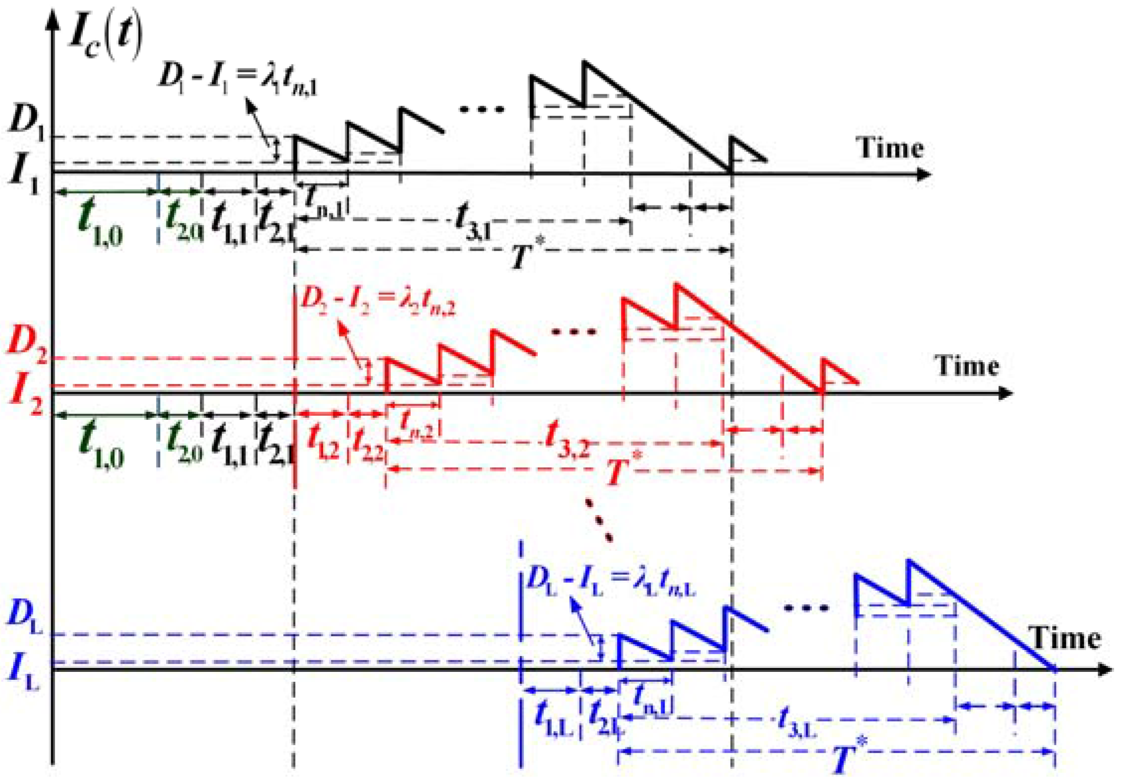
This study incorporates component commonality, postponement strategy, and quality assurance into a two-stage multi-product fabrication-distribution EPQ-based system. It is assumed that annual demands λ_i for different products L (where i = 1, 2, …, L) need to be satisfied. These L end products share a common intermediate part and are fabricated by a two-stage process. The first stage produces common components for L different products and the second stage manufactures in sequence L customized end products with the aim of maximizing machine utilization. The objectives of this study are to minimize the total production-inventory costs and shorten replenishment cycle time. In stage one, the common intermediate component is produced at a rate of P_1,0, it follows that L different customized end products are fabricated in sequence and under a common production cycle time policy (see Figure 1), at a production rate of P_1,i in stage two (where i = 1, 2, …, L). All items produced are screened and the inspection cost per item is included in the unit production cost C_i. As described by most of the realistic production systems, the processes in each stage (either for the common intermediate part or for the end products) may randomly produce x_i portion of defective items at a production rate d_1,i; hence, d_1,i = P_1,i x_i (where i = 0, 1, 2, …, L; and i = 0 denotes that it is for the production of common intermediate part in stage one).

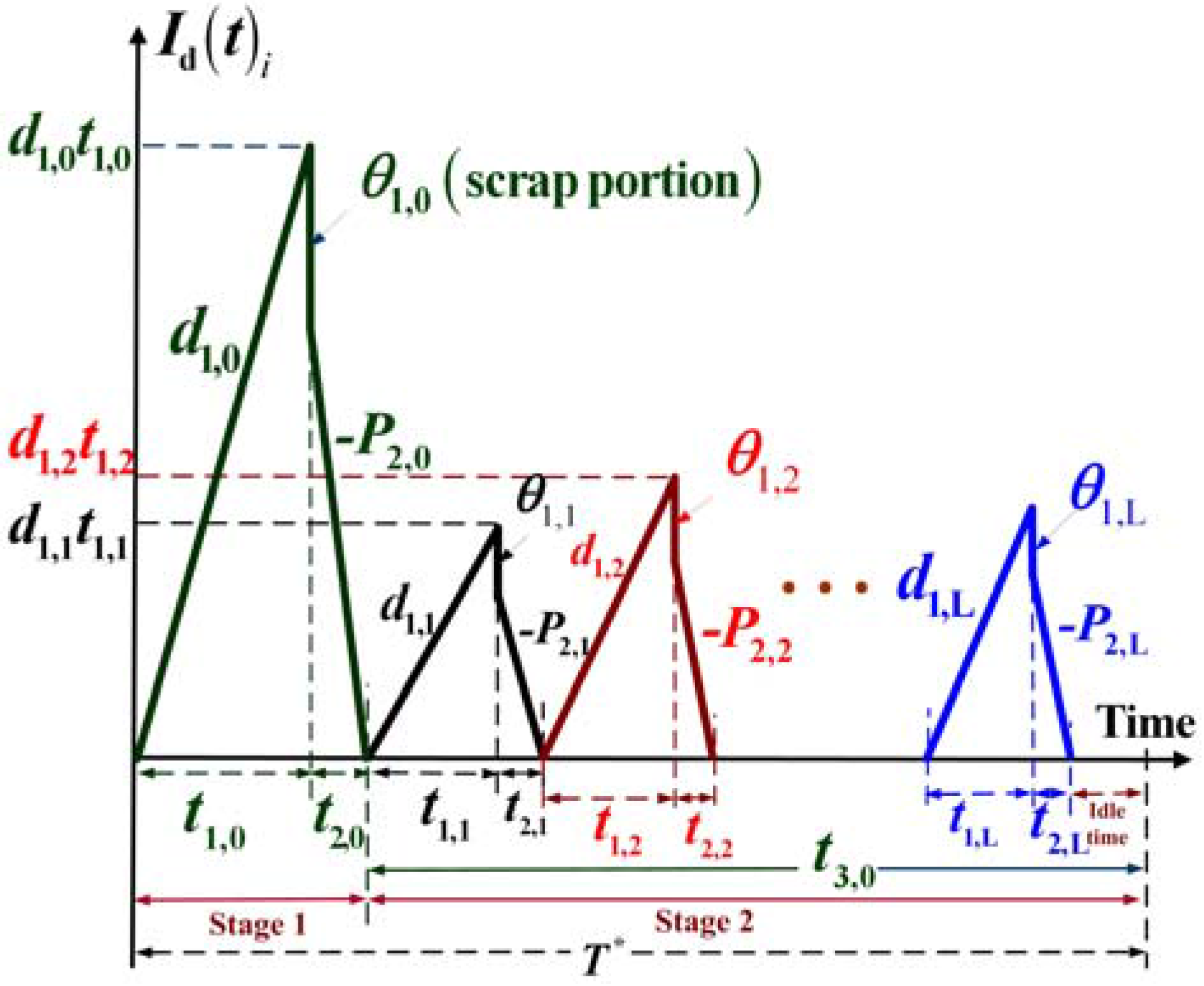
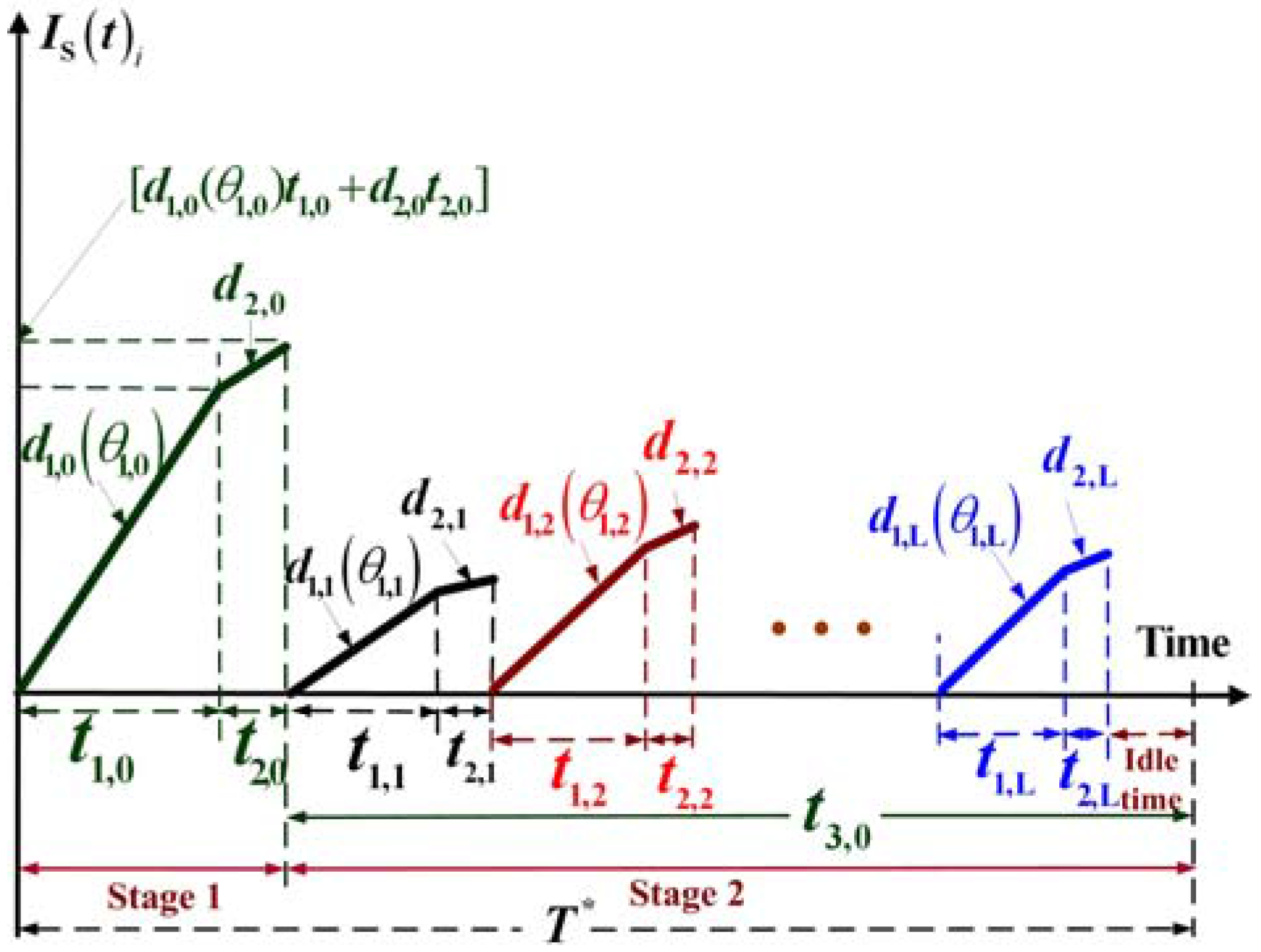
It is further assumed that after the inspection, defective items fall into two groups: a θ_1,i portion of them is the scrap (where 0 ≤ θ_1,i ≤ 1) and the other (1 – θ_1,i) portion is considered to be rework-able. In the production cycle, when regular production processes are finished, rework processes start immediately at a rate of P_2,i (where again i = 0, 1, 2, …, L). The reworking itself is not perfect either, it is assumed that a portion θ_2,i (where 0 ≤ θ_2,i ≤ 1) of reworked items fails and becomes scrap (see Figure 2). Vendor’s on-hand inventory level of scrap items in both stages of the proposed system is illustrated in Figure 3, and under the ordinary assumption of the EPQ model without shortages, the constant production rate P_1,i must be larger than the sum of demand rate λ_i and production rate of defective items d_1,i. That is: (P_1,i – d_1,i – λ_i) > 0 for i = 0, 1, 2, …, L; or (1 – x_i – λ_i/P_1,i) > 0.

In the second stage, upon completion of the rework process (t_2,i) of each end product i, fixed quantity n installments of the finished batch are distributed to the customers, at a fixed interval of time during the production downtime t_3,i (see Figure 1). Additional notation used in this study includes:

T = production cycle length, one of the decision variables,

n = the number of fixed quantity installments of the finished batch to be delivered to the customers, the other decision variable,

α = common intermediate part’s completion rate as compared to the finished product,

E[T] = the expected production cycle length,

TC(T, n) = total production-inventory-delivery cost per production cycle,

E[TC(T, n)] = the expected production-inventory-delivery cost per production cycle,

E[TCU(T, n)] = the long-run average system costs per unit time for the proposed model.

The following parameters are adopted in both stages of the proposed system (where i = 0, 1, 2, …, L, and i = 0 denotes the time during the production of the common intermediate part in the stage one):

Q_i = production lot size for product i in each production cycle,

φ_i = total scrap rate per cycle for product i, (where 0 ≤ φ_i ≤ 1),

K_i = production setup cost for product i in each production cycle,

C_i = unit production cost for product i,

h_1,i = unit holding cost for product i,

h_2,i = holding cost per reworked item for product i,

C_R,i = unit reworking cost for product i,

C_S,i = disposal cost per scrap item for product i,

h_4,i = unit holding cost for safety stocks stored at producer’s side,

t_1,i = production uptime for product i in each production cycle,

t_2,i = the reworking time for product i in each production cycle,

t_3,i = delivery time for product i in each production cycle,

H_1,i = maximal level of perfect quality items i in the end of regular production,

H_2,i = maximal level of perfect quality items i in the end of rework process before delivery.

Other notation used specifically in stage two for the production of customized end products (where i = 1, 2, …, L) are as follows:

H_i = inventory level of common intermediate part at the time of producing end product i,

K_1,i = fixed delivery cost per shipment for product i,

C_T,i = unit delivery cost for product i,

t_n,i = a fixed interval of time between each installment of finished items of product i to be delivered to customer during downtime t_3,i,

I_c(t)_i = on-hand inventory level of finished product i at time t, at customer’s side,

h_3,i = unit holding cost for stock stored at customer’s side.

2.2. Formulations

In order to meet annual demand λ_i of the customized product i during a production cycle, the following equations must be satisfied:

$$Q_i=\frac{{\lambda }_{i}T}{1-{\phi }_{i}E\left[x_i\right]}fori=1,2,\dots ,L$$

(1)

where

$$T=t_{1,i}+t_{2,i}+t_{3,i}fori=0,1,2,\dots ,L$$

(2)

$${\phi }_i={\theta }_{1,i}+{\theta }_{2,i}(1-{\theta }_{1,i})fori=0,1,2,\dots L$$

(3)

In stage one, the production lot size of common intermediate parts highly depends on the sum of annual demands of L different products to be made in stage two, hence from Equation (1) we have

$${\displaystyle \sum _{i=1}^L{Q}_i}={\lambda }_{0}T$$

(4)

$$Q_0=\frac{{\displaystyle \sum _{i=1}^L{Q}_i}}{1-{\phi }_{0}E\left[x_0\right]}$$

(5)

$$H_{1,0}=t_{1,0}\left(P_{1,0}-d_{1,0}\right)$$

(6)

$$t_{1,0}=\frac{Q_0}{P_{1,0}}=\frac{H_{1,0}}{P_{1,0}-d_{1,0}}$$

(7)

$$H_{2,0}=H_{1,0}+\left(P_{2,0}-d_{2,0}\right)t_{2,0}$$

(8)

$$t_{2,0}=\frac{x_0{Q}_0\left(1-{\theta }_{1,0}\right)}{P_{2,0}}=\frac{d_{1,0}{t}_{1,0}\left(1-{\theta }_{1,0}\right)}{P_{2,0}}=\frac{H_{2,0}-H_{1,0}}{P_{2,0}-d_{2,0}}$$

(9)

$$H_1=H_{2,0}-Q_1$$

(10)

$$H_i=H_{\left(i-1\right)}-Q_{i}fori=2,3,\mathrm{\dots },L$$

(11)

$$H_L=H_{\left(L-1\right)}-Q_L=0$$

(12)

$$H_{2,0}={\displaystyle \sum _{i=1}^L{Q}_i}$$

(13)

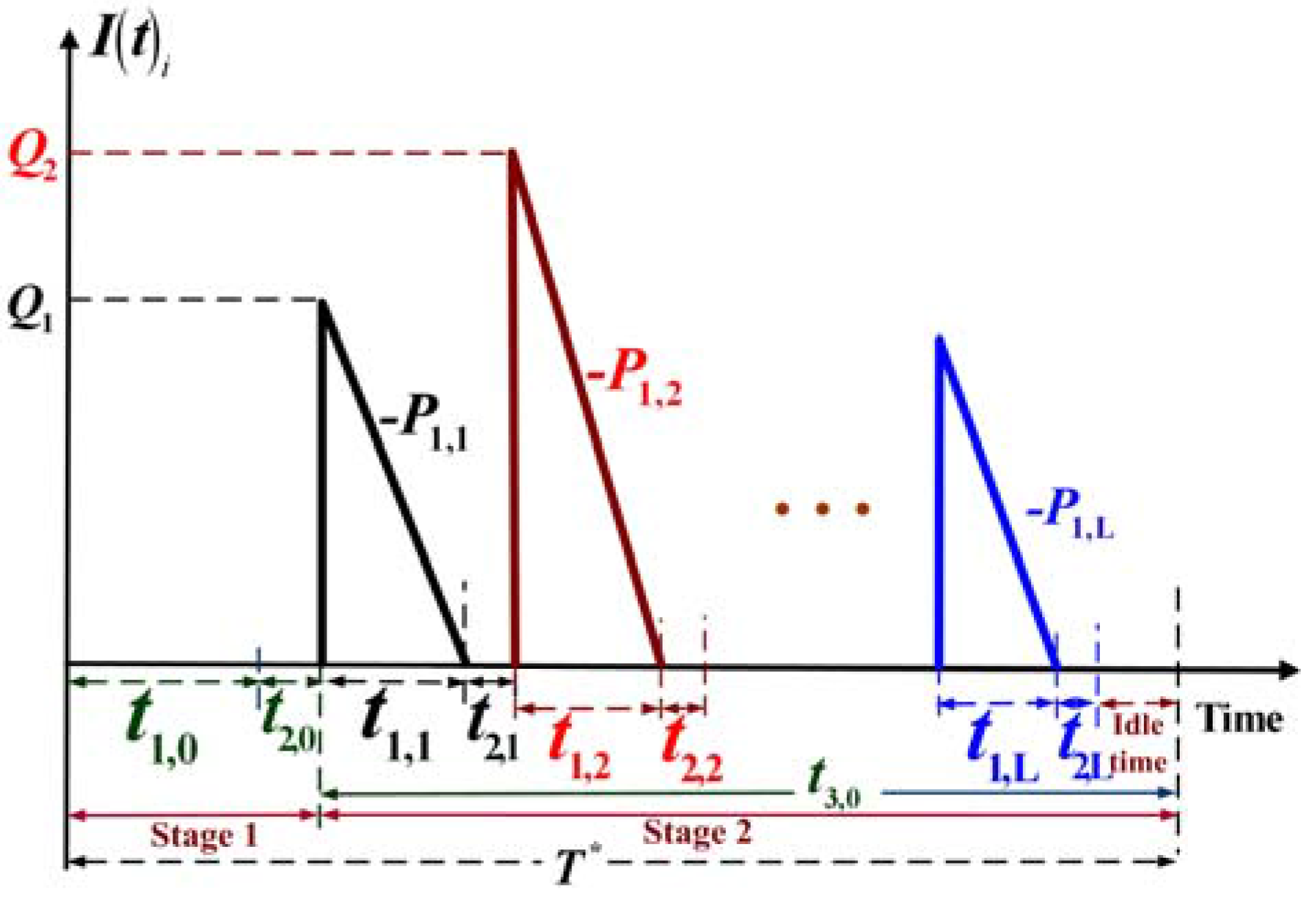
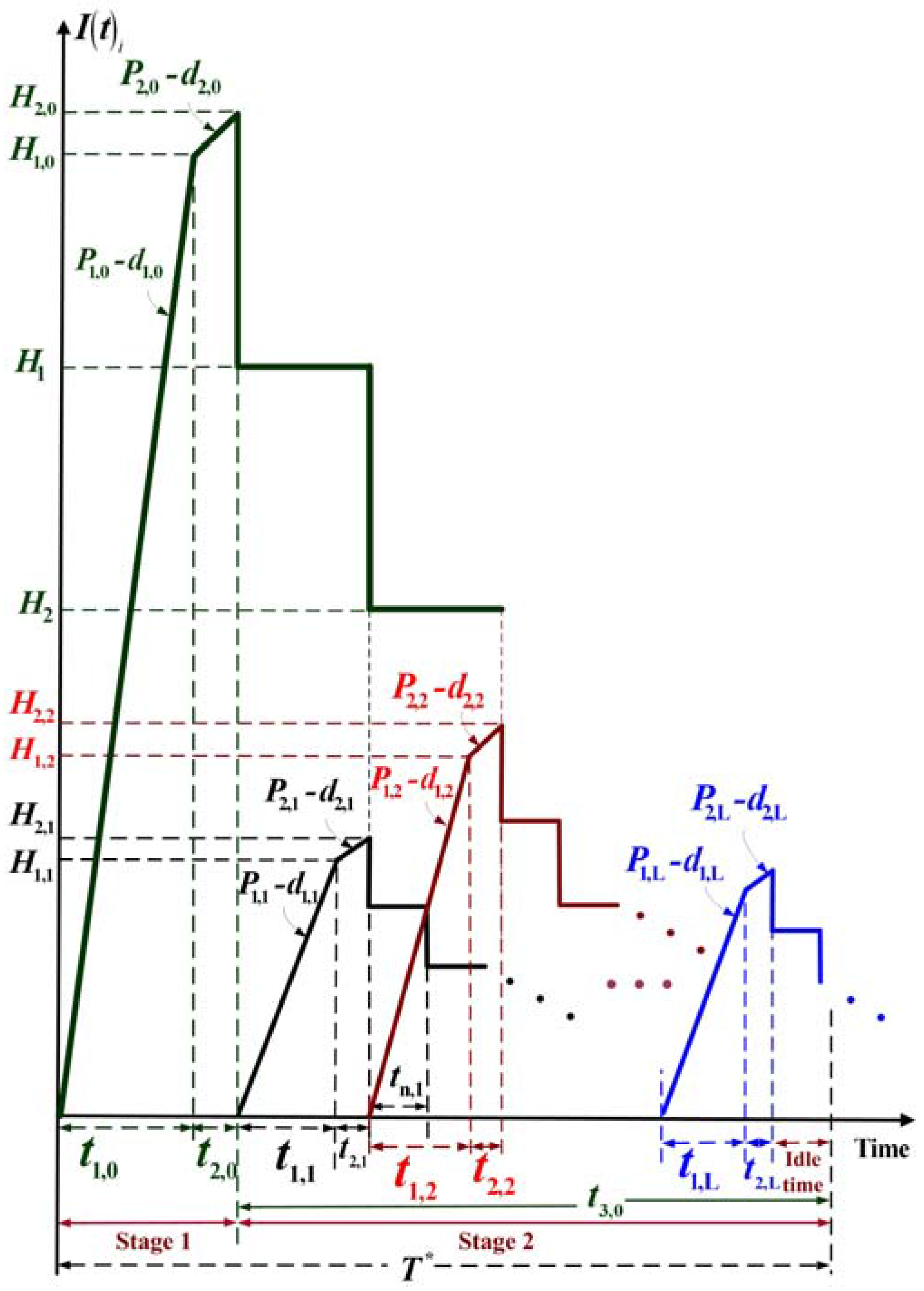
The on-hand inventory level of common intermediate parts waiting to be fabricated into end products in stage two of the proposed system is depicted in Figure 4. In stage two, from Figure 1 to Figure 4 we observe the following formulas:

$$Q_i=P_{1,i}\left(t_{1,i}\right)fori=1,2,\dots ,L$$

(14)

$$H_{1,i}=\left(P_{1,i}-d_{1,i}\right)t_{1,i}fori=1,2,\dots ,L$$

(15)

$$t_{1,i}=\frac{Q_i}{P_{1,i}}=\frac{H_{1,i}}{P_{1,i}-d_{1,i}}fori=1,2,\dots ,L$$

(16)

$$H_{2,i}=H_{1,i}+\left(P_{2,i}-d_{2,i}\right)t_{2,i}fori=1,2,\dots ,L$$

(17)

$$t_{2,i}=\frac{x_i{Q}_i\left(1-{\theta }_{1,i}\right)}{P_{2,i}}=\frac{d_{1,i}{t}_{1,i}\left(1-{\theta }_{1,i}\right)}{P_{2,i}}=\frac{H_{2,i}-H_{1,i}}{P_{2,i}-d_{2,i}}fori=1,2,\dots ,L$$

(18)

$$t_{3,i}=n{t}_{n,i}fori=1,2,\dots ,L$$

(19)

In any given cycle, one prerequisite condition for the proposed system is that the production facility must have sufficient capacity to produce items in both stages (including reworked and scrap items) to meet demands for all L customized products [54]. Therefore, the following condition must hold:

$$\left[\left(t_{1,0}+t_{2,0}\right)+{\displaystyle \sum _{i=1}^L\left(t_{1,i}+t_{2,i}\right)}\right]<T\mathrm{or}\left[Q_0\left(\frac{1}{P_{1,0}}+\frac{E\left[x_0\right]\left(1-{\theta }_{1,0}\right)}{P_{2,0}}\right)+{\displaystyle \sum _{i=1}^L{Q}_i\left(\frac{1}{P_{1,i}}+\frac{E\left[x_i\right]\left(1-{\theta }_{1,i}\right)}{P_{2,i}}\right)}\right]<T$$

(20)

or

$$\left\{\left(\frac{{\lambda }_0}{\left[1-{\phi }_{0}E\left[x_0\right]\right]}\right)\left[\frac{1}{P_{1,0}}+\frac{E\left[x_0\right]\left(1-{\theta }_{1,0}\right)}{P_{2,0}}\right]+{\displaystyle \sum _{i=1}^L\left(\frac{{\lambda }_i}{\left[1-{\phi }_{i}E\left[x_i\right]\right]}\right)\left[\frac{1}{P_{1,i}}+\frac{E\left[x_i\right]\left(1-{\theta }_{1,i}\right)}{P_{2,i}}\right]}\right\}<1$$

(21)

The on-hand inventory level of end products at the customer’s side during a production cycle is depicted in Figure 5. We can observe the following formulas directly from Figure 1 and Figure 5:

$$D_i=\frac{H_{2,i}}{n}fori=1,2,3,\mathrm{\dots },L$$

(22)

$$I_i=D_i-{\lambda }_i{t}_{n,i}fori=1,2,3,\mathrm{\dots },L$$

(23)

$$n{I}_i={\lambda }_i\left(t_{1,i}+t_{2,i}\right)fori=1,2,3,\mathrm{\dots },L$$

(24)

In stage one, the inventory holding costs for common intermediate parts (including perfect quality and defective items) during t_1,0 t_2,0, and t_3,0 are (see Figure 1 and Figure 2)

$$h_{1,0}\left[\frac{H_{1,0}{t}_{1,0}}{2}+\frac{\left(H_{2,0}+H_{1,0}\right)t_{2,0}}{2}+{\displaystyle \sum _{i=1}^L{H}_i\left(t_{1,i}+t_{2,i}\right)}\right]+h_{1,0}\left[\frac{\left(d_{1,0}{t}_{1,0}\right)t_{1,0}}{2}\right]$$

(25)

In each production cycle, the holding costs for items waiting to be reworked are (see Figure 2)

$$h_{2,0}\left[\frac{d_{1,0}{t}_{1,0}\left(1-{\theta }_{1,0}\right)}{2}\left(t_{2,0}\right)\right]+{\displaystyle \sum _{i=1}^L\left[h_{2,i}\left(\frac{P_{2,i}{t}_{2,i}}{2}\right)\left(t_{2,i}\right)\right]}$$

(26)

In stage two, inventory holding cost for common intermediate parts waiting to be fabricated into end products (see Figure 4) is

$${\displaystyle \sum _{i=1}^L\left\{h_{1,i}\left[\frac{Q_i}{2}\left(t_{1,i}\right)\right]\right\}}$$

(27)

Also, in stage two, inventory holding cost for finished product i waiting to be delivered during t_3,i is

$${\displaystyle \sum _{i=1}^L\left\{h_{1,i}\left(\frac{n-1}{2n}\right)H_{2,i}{t}_{3,i}\right\}}$$

(28)

In each production cycle, the fixed and variable delivery costs are

$${\displaystyle \sum _{i=1}^L\left\{n{K}_{1,i}+C_{T,i}\left[Q_i\left(1-{\phi }_i{x}_i\right)\right]\right\}}$$

(29)

From Figure 5, the stock holding cost for finished product i stored at customers’ sides in each cycle is [7]

$${\displaystyle \sum _{i=1}^L\left\{h_{3,i}\left[\frac{n\left(D_i-I_i\right)t_{n,i}}{2}+\frac{n\left(n+1\right)}{2}{I}_i{t}_{n,i}+\frac{n{I}_i\left(t_{1,i}+t_{2,i}\right)}{2}\right]\right\}}$$

(30)

Therefore, in each production cycle, total system production-inventory-delivery cost TC(T, n) includes variable production cost, setup cost, reworking and disposal cost, holding cost, and safety stock cost for common intermediate part (in stage one); the sum of variable production costs, setup costs, reworking and disposal costs, holding costs, and safety costs for L different customized products (in stage two); and the fixed and variable delivery costs, and the holding costs for the stocks stored at customers’ side. Hence, TC(T, n) is

$$\begin{array}{cc}TC\left(T,n\right)& =\left\{\begin{array}{l}{C}_0{Q}_0+K_0+C_{R,0}\left[x_0\left(1-{\theta }_{1,0}\right)Q_0\right]+C_{S,0}\left[x_0{\phi }_0{Q}_0\right]+h_{2,0}\left(\frac{d_{1,0}{t}_{1,0}\left(1-{\theta }_{1,0}\right)}{2}\right)\left(t_{2,0}\right)\\ +h_{1,0}\left[\frac{H_{1,0}{t}_{1,0}}{2}+\frac{H_{2,0}+H_{1,0}}{2}\left(t_{2,0}\right)+\frac{d_{1,0}{t}_{1,0}}{2}\left(t_{1,0}\right)+{\displaystyle \sum _{i=1}^L{H}_i\left(t_{1,i}+t_{2,i}\right)}\right]+h_{4,0}\left(x_0{Q}_0\right)T\end{array}\right\}\\ & +{\displaystyle \sum _{i=1}^L\left\{\begin{array}{l}{C}_i{Q}_i+K_i+C_{R,i}\left[x_i\left(1-{\theta }_{1,i}\right)Q_i\right]+C_{S,i}\left[x_i{\phi }_i{Q}_i\right]+n{K}_{1,i}+C_{T,i}\left[Q_i\left(1-{\phi }_i{x}_i\right)\right]\\ +h_{1,i}\left[\frac{Q_i}{2}\left(t_{1,i}\right)+\frac{H_{1,i}{t}_{1,i}}{2}+\frac{H_{2,i}+H_{1,i}}{2}\left(t_{2,i}\right)+\left(\frac{n-1}{2n}\right)H_{2,i}{t}_{3,i}+\frac{d_{1,i}{t}_{1,i}}{2}\left(t_{1,i}\right)\right]\\ +h_{2,i}\left(\frac{P_{2,i}{t}_{2,i}}{2}\right)\left(t_{2,i}\right)+h_{3,i}\left[\frac{n\left(D_i-I_i\right)t_{n,i}}{2}+\frac{n\left(n+1\right)}{2}{I}_i{t}_{n,i}+\frac{n{I}_i\left(t_{1,i}+t_{2,i}\right)}{2}\right]\\ +h_{4,i}\left(x_i{Q}_i\right)T\end{array}\right\}}\end{array}$$

(31)

By substituting Equations (1) to (24) in Equation (31), taking randomness of defective rate into account, and with further derivation, then the long-run average system costs per unit time E[TCU(T, n)] becomes

$$\begin{array}{l}E\left[TCU\left(T,n\right)\right]=E\left[TC\left(T,n\right)\right]/E\left[T\right]=\left[C_0{\lambda }_0{E}_{0,0}+\frac{K_0}{T}+C_{R,0}{\lambda }_0\left(1-{\theta }_{1,0}\right)E_{1,0}+C_{S,0}{\lambda }_0{\phi }_0{E}_{1,0}+{\omega }_{0}T\right]\\ +{\displaystyle \sum _{i=1}^L\left\{\begin{array}{l}\left[C_i{\lambda }_i{E}_{0,i}+\frac{K_i}{T}+C_{R,i}{\lambda }_i\left(1-{\theta }_{1,i}\right)E_{1,i}+C_{S,i}{\lambda }_i{\phi }_i{E}_{1,i}+\frac{n{K}_{1,i}}{T}+C_{T,i}{\lambda }_i\right]+\frac{h_{1,i}T{{\lambda }_i}^2}{2}\left[E_{3,i}+E_{4,i}-\frac{E_{5,i}}{n}\right]\\ +\frac{h_{2,i}T{{\lambda }_i}^2{E}_{1,i}^2}{2}\left[\frac{{\left(1-{\theta }_{1,i}\right)}^2}{P_{2,i}}\right]+\frac{h_{3,i}T{{\lambda }_i}^2}{2}\left[\frac{2E_{0,i}}{P_{1,i}}+\frac{2\left(1-{\theta }_{1,i}\right)E_{1,i}}{P_{2,i}}-\frac{1}{{\lambda }_i}+\left(1+\frac{1}{n}\right)E_{5,i}\right]+T{h}_{4,i}{\lambda }_i{E}_{1,i}\end{array}\right\}}\end{array}$$

(32)

where

$$\begin{array}{l}{E}_{0,0}=\frac{1}{\left(1-{\phi }_{0}E[x_0]\right)};E_{1,0}=\frac{E[x_0]}{\left(1-{\phi }_{0}E[x_0]\right)};E_{0,j}=\frac{1}{\left(1-{\phi }_{j}E[x_j]\right)}for\mathrm{j}=1,\dots \dots ,i;\\ {\omega }_0=\left\{\begin{array}{l}\frac{h_{1,0}{\lambda }_0^2{\left(E_{0,0}\right)}^2}{2}\left[\frac{1}{P_{1,0}}+\frac{2E\left[x_0\right]\left(1-{\theta }_{1,0}\right)\left(1-E\left[x_0\right]\right)}{P_{2,0}}+\frac{E{\left[x_0\right]}^2{\left(1-{\theta }_{1,0}\right)}^2\left(1-{\theta }_{2,0}\right)}{P_{2,0}}\right]+h_{4,0}{\lambda }_0{E}_{1,0}\\ +\frac{h_{2,0}{\lambda }_0^2{\left(E_{1,0}\right)}^2}{2}\left[\frac{{\left(1-{\theta }_{1,0}\right)}^2}{P_{2,0}}\right]+h_{1,0}{\displaystyle \sum _{i=1}^L\left\{\left(\frac{{\lambda }_i{E}_{0,i}}{P_{1,i}}+\frac{{\lambda }_i\left(1-{\theta }_{1,i}\right)E_{1,i}}{P_{2,i}}\right)\left[{\displaystyle \sum _{i=1}^L\left({\lambda }_i{E}_{0,i}\right)-{\displaystyle \sum _{j=1}^i\left({\lambda }_j{E}_{0,j}\right)}}\right]\right\}}\end{array}\right\};\\ E_{0,i}=\frac{1}{\left(1-{\phi }_{i}E[x_i]\right)};E_{1,i}=\frac{E[x_i]}{\left(1-{\phi }_{i}E[x_i]\right)};\mathrm{and}{E}_{2,i}=\left(1-{\theta }_{1,i}\right)\left(1-{\theta }_{2,i}\right)fori=1,2,\dots ,L;\\ E_{3,i}=\left[\frac{E_{0,i}^2}{P_{1,i}}+\frac{\left(1-E\left[x_i\right]\right)\left(1-{\theta }_{1i}\right)E_{0,i}{E}_{1,i}}{P_{2,i}}\right]fori=1,2,\dots ,L;\\ E_{4,i}=\left[\frac{1-E\left[x_i\right]}{{\lambda }_i}{E}_{0,i}+\frac{E_{2,i}{E}_{1,i}}{{\lambda }_i}+\frac{E_{0,i}{E}_{1,i}}{P_{1,i}}\left[1-E_{2,i}\right]\right]fori=1,2,\dots ,L;\\ E_{5,i}=\left[E_{4,i}-E_{3,i}-\frac{\left(1-{\theta }_{1,i}\right)E_{2,i}{E}_{1,i}^2}{P_{2,i}}\right]fori=1,2,\dots ,L\end{array}$$

(33)

3. Results

The Optimal Fabrication-Distribution Policy

With the intention of deriving optimal fabrication-distribution policy, we must first prove the convexity of the expected system cost function E[TCU(T, n)]. Applying Hessian matrix equations [55] we have (for details please refer to Appendix A)

$$\left[\begin{array}{cc}T& n\end{array}\right]\cdot \left(\begin{array}{cc}\frac{{\partial }^{2}E\left[TCU\left(T,n\right)\right]}{\partial T^2}& \frac{{\partial }^{2}E\left[TCU\left(T,n\right)\right]}{\partial T\partial n}\\ \frac{{\partial }^{2}E\left[TCU\left(T,n\right)\right]}{\partial T\partial n}& \frac{{\partial }^{2}E\left[TCU\left(T,n\right)\right]}{\partial n^2}\end{array}\right)\cdot \left[\begin{array}{c}T\\ n\end{array}\right]=\frac{2K_0}{T}+{\displaystyle \sum _{i=1}^L\frac{2K_i}{T}}>0$$

(34)

Since K₀, K_i, and T are all positive, so Equation (34) is positive. Therefore, E[TCU(T, n)] is a strictly convex function for all T and n different from zero. In order to concurrently determine the production-shipment policy for the proposed system, we can solve the linear system of the first derivatives of E[TCU(T, n)] with respect to T and n, respectively, by setting these partial derivatives equal to zero. With further derivations we obtain

$$T^{*}=\sqrt{\frac{K_0+{\displaystyle \sum _{i=1}^L\left(K_i+n{K}_{1,i}\right)}}{{\omega }_0+{\displaystyle \sum _{i=1}^L\left\{\begin{array}{l}\frac{h_{1,i}{{\lambda }_i}^2}{2}\left[E_{3,i}+E_{4,i}-\frac{E_{5,i}}{n}\right]+\frac{h_{2,i}{{\lambda }_i}^2{E}_{1,i}^2}{2}\left[\frac{{\left(1-{\theta }_{1,i}\right)}^2}{P_{2,i}}\right]+h_{4,i}{\lambda }_i{E}_{1,i}\\ +\frac{h_{3,i}{{\lambda }_i}^2}{2}\left[\frac{2E_{0,i}}{P_{1,i}}+\frac{2\left(1-{\theta }_{1,i}\right)E_{1,i}}{P_{2,i}}-\frac{1}{{\lambda }_i}+\left(1+\frac{1}{n}\right)E_{5,i}\right]\end{array}\right\}}}}$$

(35)

and

$$n^{*}=\sqrt{\frac{\left(K_0+{\displaystyle \sum _{i=1}^L{K}_i}\right){\displaystyle \sum _{i=1}^L\left[\frac{{{\lambda }_i}^2}{2}\left(h_{3,i}-h_{1,i}\right)E_{5,i}\right]}}{\left({\displaystyle \sum _{i=1}^L{K}_{1i}}\right)\left\{{\omega }_0+{\displaystyle \sum _{i=1}^L\left\{\begin{array}{l}\frac{h_{1,i}{{\lambda }_i}^2}{2}\left(E_{3,i}+E_{4,i}\right)+\frac{h_{2,i}{{\lambda }_i}^2{E}_{1,i}^2}{2}\left[\frac{{\left(1-{\theta }_{1,i}\right)}^2}{P_{2,i}}\right]+h_{4,i}{\lambda }_i{E}_{1,i}\\ +\frac{h_{3,i}{{\lambda }_i}^2}{2}\left[\frac{2E_{0,i}}{P_{1,i}}+\frac{2\left(1-{\theta }_{1,i}\right)E_{1,i}}{P_{2,i}}-\frac{1}{{\lambda }_i}+E_{5,i}\right]\end{array}\right\}}\right\}}}$$

(36)

4. Numerical Applications

To demonstrate a practical use of the aforementioned research results, we provide a numerical example in this section. Consider five customized end products with annual demand rates λ_i of 3000, 3200, 3400, 3600, and 3800 units satisfied by a manufacturer with one piece of production equipment, and these five end products share a common intermediate part that is halfway done (i.e., α = 0.5). Consider a multi-item system without postponing its production processes for end products [7]: the production setup costs K_i for the end products are $17,000, $17,500, $18,000, $18,500, and $19,000, respectively; unit manufacturing costs C_i are $80, $90, $100, $110, and $120, respectively; unit reworking costs C_R,i are $50, $55, $60, $65, and $70, respectively; and unit scrap costs C_S,i are $20, $25, $30, $35, and $40, respectively. The random defective rates x_i follow the uniform distribution over the intervals [0, 0.05], [0, 0.10], [0, 0.15], [0, 0.20], and [0, 0.25], respectively; annual production rates P_1,i for the end products are 58,000, 59,000, 60,000, 61,000, and 62,000 units, respectively; and the reworking rates P_2,i for the end products are 46,400, 47,200, 48,000, 48,800, and 49,600 units, respectively.

Assume a linear relationship in proportion to the completion rate α applied to our proposed two-stage production scheme. Therefore, in stage one we have P_1,0 = 120,000 and P_2,0 = 96,000 (where P_1,0 = (1/α) * (the mean of P_1,i’s), and P_2,0 = (1/α) * (the mean of P_2,i’s)). We also have the linear-based setup cost K₀ = $8500; unit fabrication cost C₀ = $40, unit reworking cost C_R,0 = $25, unit scrap cost C_S,0 = $10, unit holding cost h_1,0 = $5 (let h_4,0 = h_1,0), holding cost per reworked item h_2,0 = $15, defect rate x₀= [0, 0.04], scrap rate during regular production θ_1,0 = 0.20, and scrap rate during the reworking process θ_2,0 = 0.20.

In stage two, the following cost related parameters result from the same linear relationship with α: K_i = $8500, $9000, $9500, $10,000, and $10,500, respectively; C_,i = $40, $50, $60, $70, and $80, respectively; unit reworking costs C_R,i = $25, $30, $35, $40, and $45, respectively; unit scrap costs C_S,i = $10, $15, $20, $25, and $30, respectively. The random defective rates x_i follow the uniform distribution over the intervals [0, 0.01], [0, 0.06], [0, 0.11], [0, 0.16], and [0, 0.21], respectively. However, we assume that production and reworking rates P_1,i and P_2,i in the proposed system have 1/α linear relationships with their original rates. Specifically, we set P_1,i = 112,258, 116,066, 120,000, 124,068, and 128,276 units, respectively; and P_2,i = 89,806, 92,852, 96,000, 99,254, and 102,621 units, respectively (where P_1,i = 1/(1/P_1,i – 1/P_1,0) and P_2,i = 1/(1/P_2,i – 1/P_2,0)). The following parameters remain the same: unit holding cost (e.g. for perfect, defective, or safety items) per unit time h_1,i are $10, $15, $20, $25, and $30, respectively; holding cost per reworked item h_2,i are $30, $35, $40, $45, and $50, respectively; fixed delivery costs per shipment K_1i are $1800, $1900, $2000, $2100, and $2200, respectively; unit delivery costs C_T,i are $0.1, $0.2, $0.3, $0.4, and $0.5 respectively; unit holding costs h_3,i at the customers’ end are $70, $75, $80, $85, and $90, respectively; scrap rates during regular production θ_1,i = 0.10, 0.15, 0.20, 0.25, and 0.30, respectively; and scrap rates during the reworking processes θ_2,i = 0.10, 0.15, 0.20, 0.25, and 0.30, respectively.

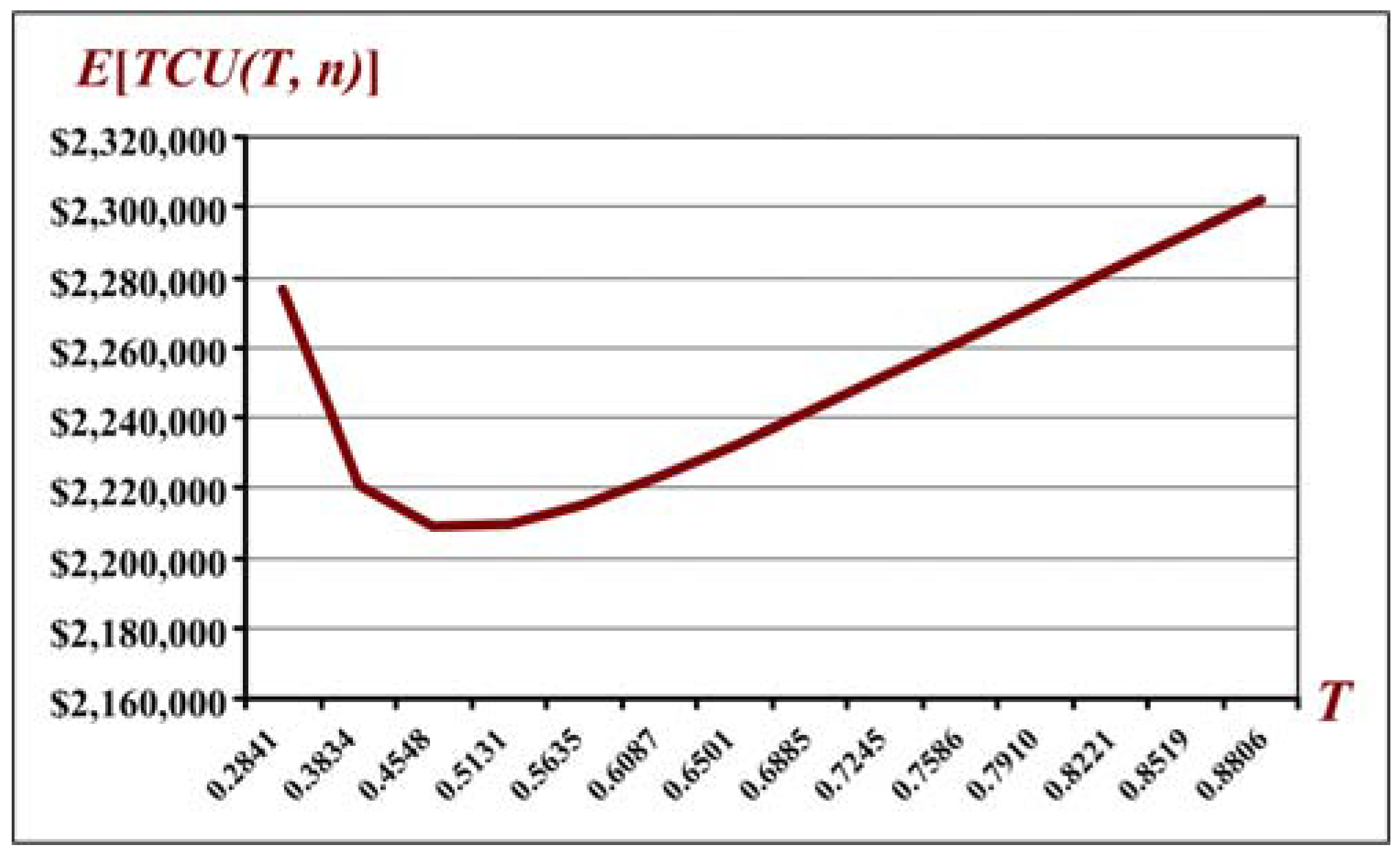
Applying Equation (3), we find the overall scrap rate for stage one, φ_i equal to 0.36. By computing Equations (1) and (4), we also obtain the annual demand for common intermediate parts λ₀ as 17,570. By calculating Equations (35), (36), and (32), we find the optimal number of deliveries n* = 3, the optimal production cycle time T* = 0.4600 (years), and the long-run average system costs per unit time E[TCU(T*, n*)] = $2,209,201. Figure 6 illustrates the behavior of E[TCU(T, n)] with respect to common production cycle time T.

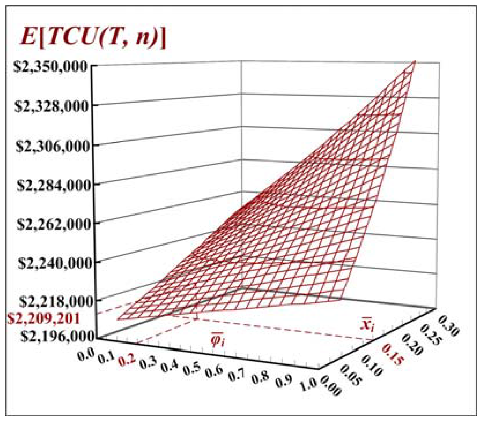
Figure 7 depicts the joint effects of variations of the expected average defective rates and the expected average scrap rates on the long-run average system costs E[TCU(T, n)]. It is noted that as both the expected average defective rates and the expected average scrap rates increase, the long-run average system costs E[TCU(T, n)] increase significantly. Such an analytical result provides the production planner/controller with valuable information of ‘quality cost in production’.

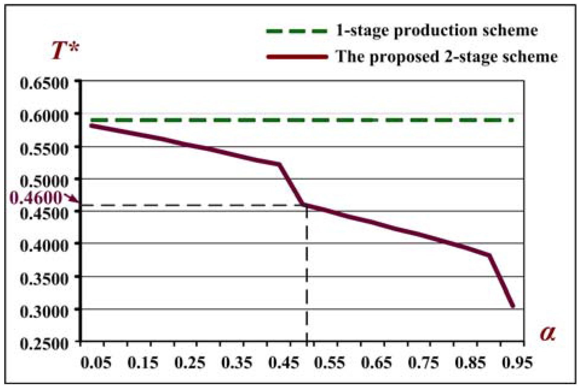
The effects of variations of the common intermediate part’s completion rate α on optimal production cycle time T* is shown in Figure 8. As the completion rate α increases, the optimal cycle time T* decreases significantly. It is also noted that the production cycle time is reduced by 22.11% at α = 0.5 (i.e., it has dropped from 0.5906 to 0.4600 years) as compared to that in a prior study which adopted a single-stage production scheme. Such a result indicates that the proposed two-stage multi-item production scheme with delayed differentiation provides a shorter production cycle time (or faster response time) than that in a conventional one-stage multi-item production system [7].

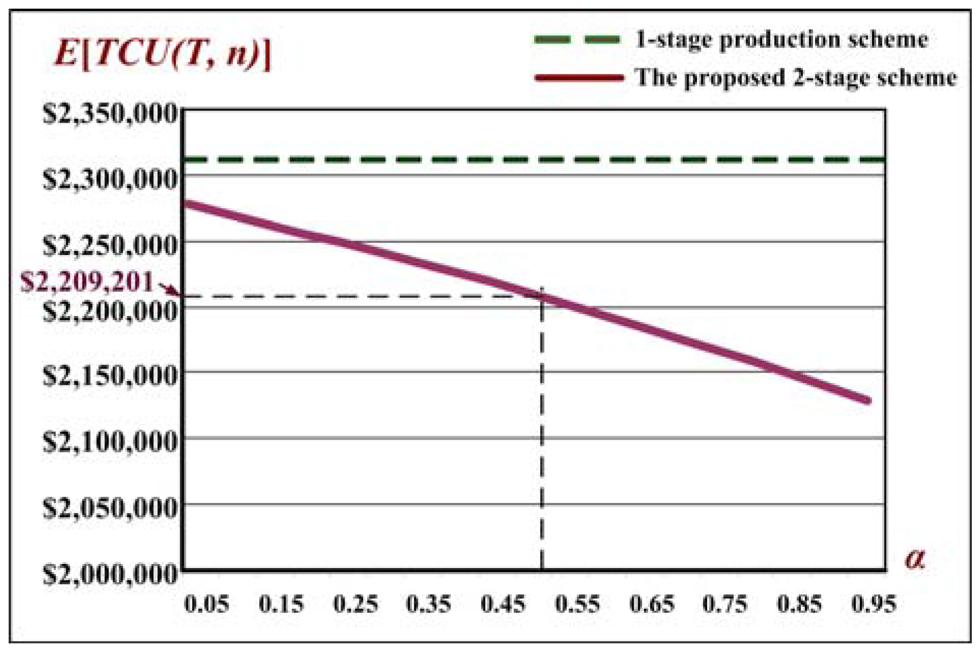
Figure 9 depicts the behavior of E[TCU(T, n)] with respect to common intermediate part’s completion rate α. The illustration demonstrates that as the completion rate α increases, the long-run expected system cost E[TCU(T, n)] decreases. It is also noted that the proposed study realized an overall system cost savings of 4.63% at α = 0.5 (i.e., system costs decreased from $2,316,483 to $2,209,201) as compared to that in a prior study which used a single-stage production scheme. This result implies that the proposed two-stage multi-product production scheme with delayed differentiation is a considerably beneficial model to producers who must satisfy demands for multiple products that share a common intermediate part.

Investigation of Nonlinear Cost Related Parameters

Suppose that the relationship between the practical fabrication cost of the common intermediate part (or the value of the work-in-process) and its completion rate α is not linear. We use the following analysis to demonstrate that the proposed model is capable of analyzing any given nonlinear relationship between the relevant costs of a common intermediate part and its completion rate α. For example, assume a nonlinear relationship of ‘α^(1/3)’ between the common intermediate part’s relevant costs and α. Hence, C₀ = [α^(1/3)]C₁ = [(0.5)^(1/3)]$80 = $63 and it is noted that the common part has a higher production cost (value) than that in the linear relationship case (which is $40). A similar computation will yield the following: K₀ = $13,493, C_R,0 = $40, C_S,0 = $16, h_1,0 = $8, h_2,0 = $24, and h_4,0 = $8.

Assuming that the values of the other variables remain the same as stated in the previous subsection, i.e., P_1,0 = 120,000, P_2,0 = 96,000, x₀= [0, 0.04], θ_1,0 = 0.20, θ_2,0 = 0.20, and φ₀ = 0.36. Therefore, in stage two the following cost parameters can be obtained accordingly: K_i = $3507, $4007, $4507, $5007, and $5507, respectively; C_,i = $17, $27, $37, $47, and $57, respectively; unit reworking costs C_R,i are $10, $15, $20, $25, and $30, respectively; unit scrap costs C_S,i are $4, $9, $14, $19, and $24, respectively. The random defect rates x_i follow the uniform distribution over the intervals [0, 0.01], [0, 0.06], [0, 0.11], [0, 0.16], and [0, 0.21], respectively; scrap rates θ_1,i = 0.10, 0.15, 0.20, 0.25, and 0.30, respectively; and θ_2,i = 0.10, 0.15, 0.20, 0.25, and 0.30, respectively. We apply Equations (35), (36), and (32) to obtain the optimal number of deliveries n* = 3, the optimal common production cycle time T* = 0.3991 (years), and the long-run average system costs per unit time E[TCU(T*, n*)] = $2,163,075. It is noted that in this nonlinear case, production cycle time T* is shortened by 13.24% and the expected system costs E[TCU(T, n)] is decreased by 2.09% as compared to that in the case of the linear one.

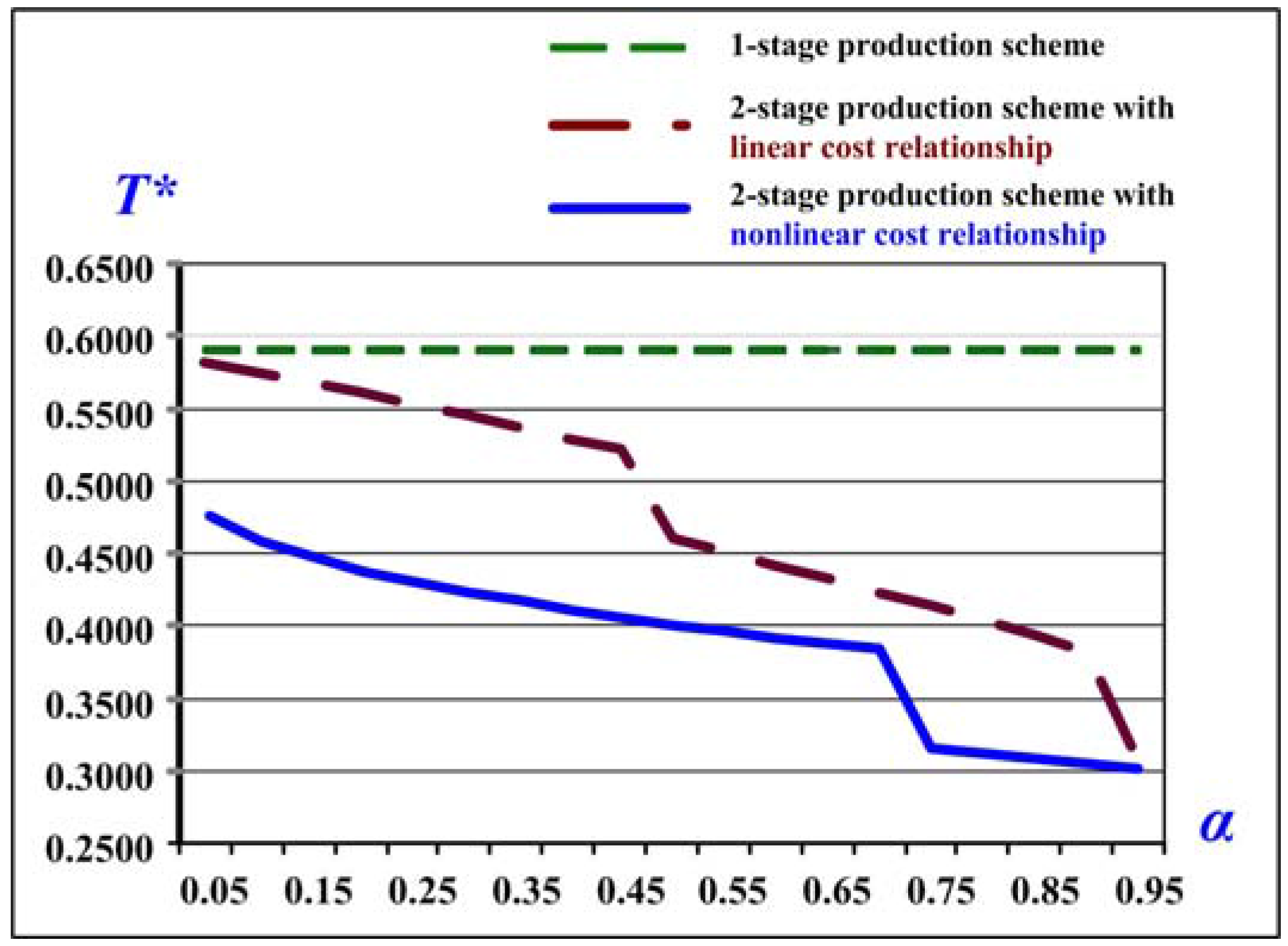
Figure 10 shows the behavior of the optimal production cycle time T* with respect to common intermediate part’s completion rate α under both linear and nonlinear relationships. In the nonlinear relationship between a common part’s relevant costs and its completion rate, as the completion rate α increases, the optimal production cycle time T* decreases significantly, indicating that the proposed two-stage multi-item production scheme with delayed differentiation provides a shorter production cycle time (or response time) than that in a conventional one-stage multi-item production system [7]. The analytical results also reveal that if the common intermediate part’s relevant costs are higher (e.g., have a nonlinear relationship α^(1/3) rather than linear one), then the optimal production cycle time T* decreases significantly compared to the linear case.

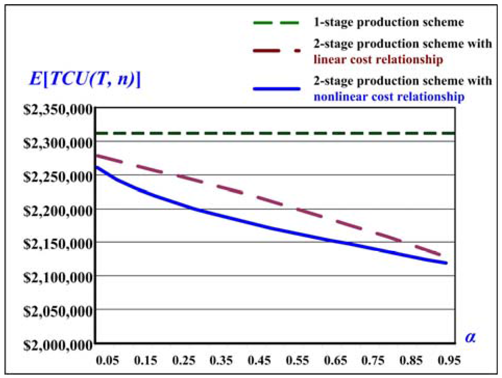
Figure 11 illustrates the behavior of E[TCU(T, n)] with respect to the common intermediate part’s completion rate α under both linear and nonlinear relationships. It is noted that in the nonlinear relationship between a common part’s relevant costs and its completion rate, as the completion rate α increases, the long-run expected system cost E[TCU(T, n)] decreases. The proposed two-stage multi-product production scheme with delayed differentiation is therefore a considerably beneficial model to producers who must satisfy demand for multiple products that share a common intermediate part. The analytical results also demonstrate that if the common intermediate part’s relevant costs are higher (e.g., have a nonlinear relationship α^(1/3) rather than linear one), then the expected system cost E[TCU(T, n)] decreases significantly compared to the linear case.

In the aforementioned numerical examples, the selected parameters’ values are general, within reasonable assumptions and they are not chosen only for this demonstration. That is, one can apply any practical data from the real world manufacturing firms to the proposed model and obtain the same or similar results as illustrated in Figure 6, Figure 7, Figure 8, Figure 9, Figure 10 and Figure 11.

In summary, major findings of our research results and numerical analyses include (1) the convexity of system cost function and the effect of optimal production cycle time on the system cost; (2) joint effects of the expected average defective rates and average scrap rates on the expected system cost; (3) effect of different common part’s completion rates on the optimal production cycle time; (4) effect of different common part’s completion rates on the expected system cost; (5) the behavior of optimal production cycle time with respect to common part’s completion rate α under both linear and nonlinear relationships; and (6) the behavior of system cost with respect to common part’s completion rate α under both linear and nonlinear relationships.

5. Conclusions

Motivated to assist managers of manufacturing firms in gaining competitive advantages, maximizing machine utilization, and reducing overall quality and fabrication-distribution costs, this study explores a multi-product fabrication-distribution problem with component commonality, postponement, and quality assurance. A two-stage single-machine production scheme with the reworking of repairable nonconforming items is proposed. The first stage of the proposed system fabricates common intermediate components for all products, and the second stage produces finished products under a common production cycle time policy. The mathematical modeling and optimization techniques enable us to derive the closed-form optimal fabrication-distribution policy that minimize the expected total system costs for the proposed system. A numerical example is provided to show practical use of the obtained decision (see Figure 6 and Figure 7). Through analytical and numerical comparisons, we gain insights and demonstrate that the proposed production scheme is beneficial in terms of reduced cycle time (Figure 8) and cost savings (Figure 9) as compared to that in a single-stage production scheme. Further analysis also reveals that when the common intermediate component’s value is higher (e.g., it has a nonlinear relationship α^(1/3) with its completion rate, rather than the linear one), both the production cycle time (Figure 10) and expected system costs (Figure 11) are reduced significantly compared to that in the linear case.

In summary, the research results of this study can help management better understand, plan, and control real-world vendor-buyer integrated multi-product systems with component commonality, postponement strategy, and quality assurance. It enables manufacturers to gain more competitive advantages in the turbulent global business environment. To study the effect of stochastic production rate on the operational policy to the problem will be an interesting topic for future study.

References

Bergstrom, G.L.; Smith, B.E. Multi-item Production Planning. An Extension of the HMMS Rules. Manag. Sci.1970, 16, 614–629. [Google Scholar] [CrossRef]
Gaalman, G.J. Optimal Aggregation of Multi-item Production Smoothing Models. Manag. Sci.1978, 24, 1733–1739. [Google Scholar] [CrossRef]
Zipkin, P.H. Models for Design and Control of Stochastic, Multi-item Batch Production Systems. Oper. Res.1986, 34, 91–104. [Google Scholar] [CrossRef]
Golany, B.; Lev-er, A. Comparative analysis of multi-item joint replenishment inventory models. Int. J. Prod. Res.1992, 30, 1791–1801. [Google Scholar] [CrossRef]
Aragone, L.S.; Gonzalez, R.L.V. Fast computational procedure for solving multi-item single-machine lot scheduling optimization problems. J. Optim. Theory Appl.1997, 93, 491–515. [Google Scholar] [CrossRef]
Rizk, N.; Martel, A.; D’Amours, S. Multi-item dynamic production-distribution planning in process industries with divergent finishing stages. Comput. Oper. Res.2006, 33, 3600–3623. [Google Scholar] [CrossRef]
Chiu, Y.-S.P.; Chiang, K.-W.; Chiu, S.W.; Song, M.-S. Simultaneous determination of production and shipment decisions for a multi-product inventory system with a rework process. Adv. Prod. Eng. Manag.2016, 11, 141–151. [Google Scholar] [CrossRef]
Gordon, G.R.; Surkis, J. A control policy for multi-item inventories with fluctuating demand using simulation. Comput. Oper. Res.1975, 2, 91–100. [Google Scholar] [CrossRef]
Schneider, H.; Rinks, D.B. Optimal policy surfaces for a multi-item inventory problem. Eur. J. Oper. Res.1989, 39, 180–191. [Google Scholar] [CrossRef]
Viswanathan, S.; Piplani, R. Coordinating supply chain inventories through common replenishment epochs. Eur. J. Oper. Res.2001, 129, 277–286. [Google Scholar] [CrossRef]
Topan, E.; Pelin Bayindir, Z.; Tan, T. An exact solution procedure for multi-item two-echelon spare parts inventory control problem with batch ordering in the central warehouse. Oper. Res. Lett.2010, 38, 454–461. [Google Scholar] [CrossRef]
Chiu, S.W.; Sung, P.-C.; Tseng, C.-T.; Chiu, Y.-S.P. Multi-product FPR model with rework and multi-shipment policy resolved by algebraic approach. J. Sci. Ind. Res. India2015, 74, 555–559. [Google Scholar]
Haider, A.; Mirza, J. An implementation of lean scheduling in a job shop environment. Adv. Prod. Eng. Manag.2015, 10, 5–17. [Google Scholar] [CrossRef]
Chiu, Y.-S.P.; Sung, P.-C.; Chiu, S.W.; Chou, C.-L. Mathematical modeling of a multi-product EMQ model with an enhanced end items issuing policy and failures in rework. SpringerPlus2015, 4. [Google Scholar] [CrossRef] [PubMed]
Gerchak, Y.; Magazine, M.J.; Gamble, B.A. Component commonality with service level requirements. Manag. Sci.1988, 34, 753–760. [Google Scholar] [CrossRef]
Lee, H.L. Effective inventory and service management through product and process redesign. Oper. Res.1996, 44, 151–159. [Google Scholar] [CrossRef]
Al-Salim, B.; Choobineh, F. Redesign of production flow lines to postpone product differentiation. Int. J. Prod. Res.2009, 47, 5563–5590. [Google Scholar] [CrossRef]
Banerjee, A.; Sarkar, B.; Mukhopadhyay, S.K. Multiple decoupling point paradigms in a global supply chain syndrome: A relational analysis. Int. J. Prod. Res.2012, 50, 3051–3065. [Google Scholar] [CrossRef]
Collier, D.A. Aggregate safety stock levels and component part commonality. Manag. Sci.1982, 28, 1296–1303. [Google Scholar] [CrossRef]
Swaminathan, J.M.; Tayur, S.R. Models for supply chains in e-business. Manag. Sci.2003, 49, 1387–1406. [Google Scholar] [CrossRef]
Silver, E.A.; Minner, S. A replenishment decision involving partial postponement. OR Spectr.2005, 27, 1–19. [Google Scholar] [CrossRef]
Graman, G.A. A partial-postponement decision cost model. Eur. J. Oper. Res.2010, 201, 34–44. [Google Scholar] [CrossRef]
Lu, C.-C.; Tsai, K.-M.; Chen, J.-H. Evaluation of manufacturing system redesign with multiple points of product differentiation. Int. J. Prod. Res.2012, 50, 7167–7180. [Google Scholar] [CrossRef]
Taft, E.W. The most economical production lot. Iron Age1918, 101, 1410–1412. [Google Scholar]
Makis, V. Optimal lot sizing and inspection policy for an EMQ model with imperfect inspections. Nav. Res. Logist.1998, 45, 165–186. [Google Scholar] [CrossRef]
Wee, H.M.; Yu, J.; Chen, M.C. Optimal inventory model for items with imperfect quality and shortage back ordering. Omega2007, 35, 7–11. [Google Scholar] [CrossRef]
Lin, G.C.; Gong, D.-C.; Chang, C.-C. On an economic production quantity model with two unreliable key components subject to random failures. J. Sci. Ind. Res. India2014, 73, 149–152. [Google Scholar]
Pal, S.; Mahapatra, G.S.; Samanta, G.P. A production inventory model for deteriorating item with ramp type demand allowing inflation and shortages under fuzziness. Econ. Model.2015, 46, 334–345. [Google Scholar] [CrossRef]
Karunambigai, S.; Geetha, K.; Shabeer, H.A. Power Quality Improvement of Grid Connected Solar System. J. Sci. Ind. Res. India2015, 74, 354–357. [Google Scholar]
Goyal, S.K.; Gupta, Y.P. Integrated inventory models: The buyer-vendor coordination. Eur. J. Oper. Res.1989, 41, 261–269. [Google Scholar] [CrossRef]
Hill, R.M. Optimizing a production system with a fixed delivery schedule. J. Oper. Res. Soc.1996, 47, 954–960. [Google Scholar] [CrossRef]
Chen, K.-K.; Chiu, S.W. Replenishment lot size and number of shipments for EPQ model derived without derivatives. Math. Comput. Appl.2011, 16, 753–760. [Google Scholar] [CrossRef]
Yeh, T.-M.; Pai, F.-Y.; Liao, C.-W. Using a hybrid MCDM methodology to identify critical factors in new product development. Neural Comput. Appl.2014, 24, 957–971. [Google Scholar] [CrossRef]
Tseng, C.-T.; Wu, M.-F.; Lin, H.-D.; Chiu, Y.-S.P. Solving a vendor-buyer integrated problem with rework and a specific multi-delivery policy by a two-phase algebraic approach. Econ. Model.2014, 36, 30–36. [Google Scholar] [CrossRef]
Ocampo, L.A. A hierarchical framework for index computation in sustainable manufacturing. Adv. Prod. Eng. Manag.2015, 10, 40–50. [Google Scholar] [CrossRef]
Pai, F.-Y. How supplier exercised power affects the cooperative climate, trust and commitment in buyer-supplier relationships. Int. J. Bus. Excell.2015, 8, 662–673. [Google Scholar] [CrossRef]
Herui, C.; Xu, P.; Yuqi, Z. Co-Evolution Analysis on Coal-Power Industries Cluster Ecosystem Based on the Lotka-Volterra Model: A Case Study of China. Math. Comput. Appl.2015, 20, 121–136. [Google Scholar] [CrossRef]
Yu, K.-Y.; Bricker, D.L. Analysis of a markov chain model of a multistage manufacturing system with inspection, rejection, and rework. IIE Trans.1993, 25, 109–112. [Google Scholar] [CrossRef]
Grosfeld-Nir, A.; Gerchak, Y. Multistage production to order with rework capability. Manag. Sci.2002, 48, 652–664. [Google Scholar] [CrossRef]
Ma, W.-N.; Gong, D.-C.; Lin, G.C. An optimal common production cycle time for imperfect production processes with scrap. Math. Comput. Model.2010, 52, 724–737. [Google Scholar] [CrossRef]
Chiu, Y.-S.P.; Chang, H.-H. Optimal run time for EPQ model with scrap, rework and stochastic breakdowns: A note. Econ. Model.2014, 37, 143–148. [Google Scholar] [CrossRef]
Safaei, M. An integrated multi-objective model for allocating the limited sources in a multiple multi-stage lean supply chain. Econ. Model.2014, 37, 224–237. [Google Scholar] [CrossRef]
Chiu, S.W.; Huang, C.-C.; Chiang, K.-W.; Wu, M.-F. On intra-supply chain system with an improved distribution plan, multiple sales locations and quality assurance. SpringerPlus2015, 4. [Google Scholar] [CrossRef] [PubMed]
Taleizadeh, A.A.; Kalantari, S.S.; Cárdenas-Barrón, L.E. Pricing and lot sizing for an EPQ inventory model with rework and multiple shipments. TOP2016, 24, 143–155. [Google Scholar] [CrossRef]
Cárdenas-Barrón, L.E.; Treviño-Garza, G.; Taleizadeh, A.A.; Pandian, V. Determining replenishment lot size and shipment policy for an EPQ inventory model with delivery and rework. Math. Probl. Eng.2015, 2015, 595498. [Google Scholar] [CrossRef]
Treviño-Garza, G.; Castillo-Villar, K.K.; Cárdenas-Barrón, L.E. Joint determination of the lot size and number of shipments for a family of integrated vendor-buyer systems considering defective products. Int. J. Syst. Sci.2015, 46, 1705–1716. [Google Scholar] [CrossRef]
Cárdenas-Barrón, L.E. A note on models for a family of products with shelf life, and production and shortage costs in emerging markets. Int. J. Ind. Eng. Comput.2012, 3, 277–280. [Google Scholar] [CrossRef]
Cárdenas-Barrón, L.E.; Sarkar, B.; Treviño-Garza, G. Easy and improved algorithms to joint determination of the replenishment lot size and number of shipments for an EPQ model with rework. Math. Comput. Appl.2013, 18, 132–138. [Google Scholar] [CrossRef]
Ting, C.-K.; Chiu, Y.-S.P.; Chan, C.-C.H. Optimal lot sizing with scrap and random breakdown occurring in backorder replenishing period. Math. Comput. Appl.2011, 16, 329–339. [Google Scholar] [CrossRef]
Nahmias, S. Production & Operations Analysis; McGraw-Hill Inc.: New York, NY, USA, 2009. [Google Scholar]
Rardin, R.L. Optimization in Operations Research; Prentice-Hall: Upper Saddle River, NJ, USA, 1998. [Google Scholar]
Figure 1.
On-hand inventory level of perfect quality common intermediate components and finished products for a two-stage multi-product fabrication-distribution system with postponement and quality assurance.
Figure 2.
On-hand inventory level of defective items in both stages of the proposed system.
Figure 3.
On-hand inventory level of scrap items in both stages of the proposed system.
Figure 4.
On-hand inventory level of common intermediate components waiting to be fabricated into end products in stage two of the proposed system.
Figure 5.
On-hand inventory level of end products at the customer’s side during a production cycle.
Figure 6.
Long-run average system costs E[TCU(T, n)] with respect to common production cycle time T.
Figure 7.
Joint effects of variations of the expected average defective rates and expected average scrap rates on the long-run average system costs E[TCU(T, n)].
Figure 8.
Optimal production cycle time T* with respect to the common intermediate part’s completion rate α.
Figure 9.
E[TCU(T, n)] with respect to the common intermediate part’s completion rate α.
Figure 10.
Optimal production cycle time T* with respect to common intermediate part’s completion rate α under both linear and nonlinear relationships.
Figure 11.
E[TCU(T, n)] with respect to the common intermediate part’s completion rate α under both linear and nonlinear relationships.
Chiu, S.W.; Kuo, J.-S.; Chiu, V.; Chiu, Y.-S.P.