
Adjustable Bézier Curves with Simple Geometric Continuity Conditions

Abstract
:1. Introduction
2. Blending Functions
2.1. Construction of the Blending Functions
2.2. Properties of the Blending Functions
- (a)
- Degeneracy: When , the BL functions are the quartic Bernstein basis functions.
- (b)
- Non-negativity: When , for any and , we have , .
- (c)
- Normalization: For any , , and , we have .
- (d)
- Symmetry: For any , , , and , we have , and .
- (e)
- Endpoint property: For any , , and we haveAnd, for any , when , we have
- (f)
- Linear independence: For any , , and , the BL functions , are linearly independent.
- (e)
- The conclusions in (2) are obvious. We only prove (3a) and (3b). Ifwhere then
- (f)
- Let us consider the linear combinationwhere Substituting (1) into (10) and rearranging the terms, we obtain
3. Adjustable Bézier Curves
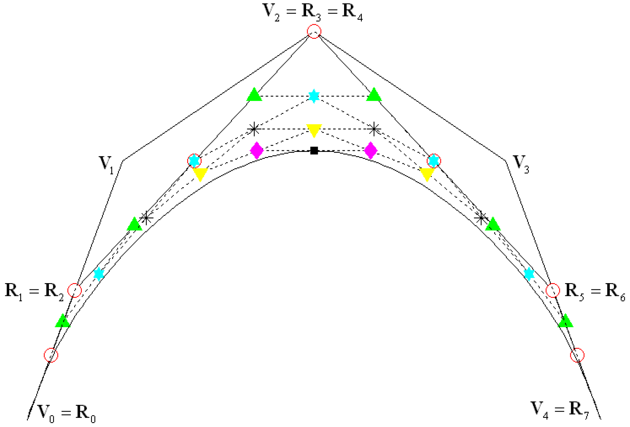
3.1. Construction of the Adjustable Bézier Curves
3.2. Properties of the Adjustable Bézier Curves
- (1)
- Convex hull property: The adjustable Bézier curves lie inside the convex hull of the control points. This is true, since the BL functions are nonnegative on and sum to 1.
- (2)
- Geometric invariance: From (13), we know that the adjustable Bézier curves are affine combinations of their control points. Thus, their shape is independent of the choice of the coordinate system.
- (3)
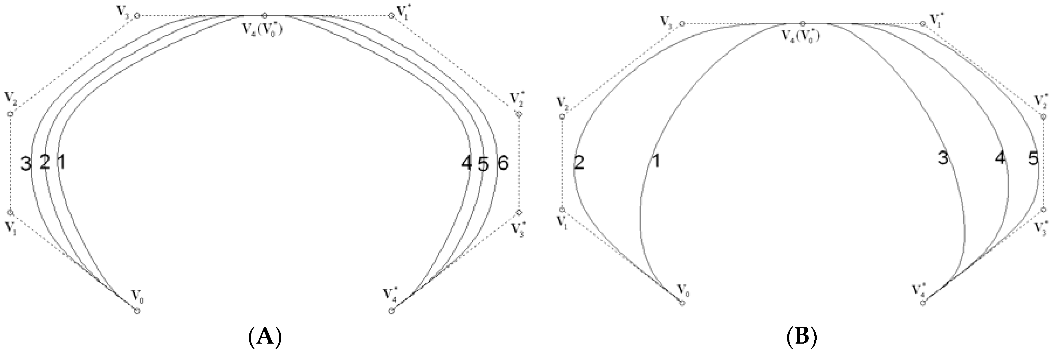
- Symmetry: The points , , and , , define two adjustable Bézier curves with the same shape but different parameterization.
- (4)
- Geometric property at the endpoints: From (2), (3) and (12) we get
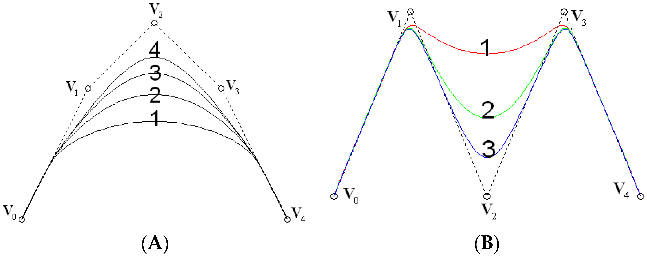
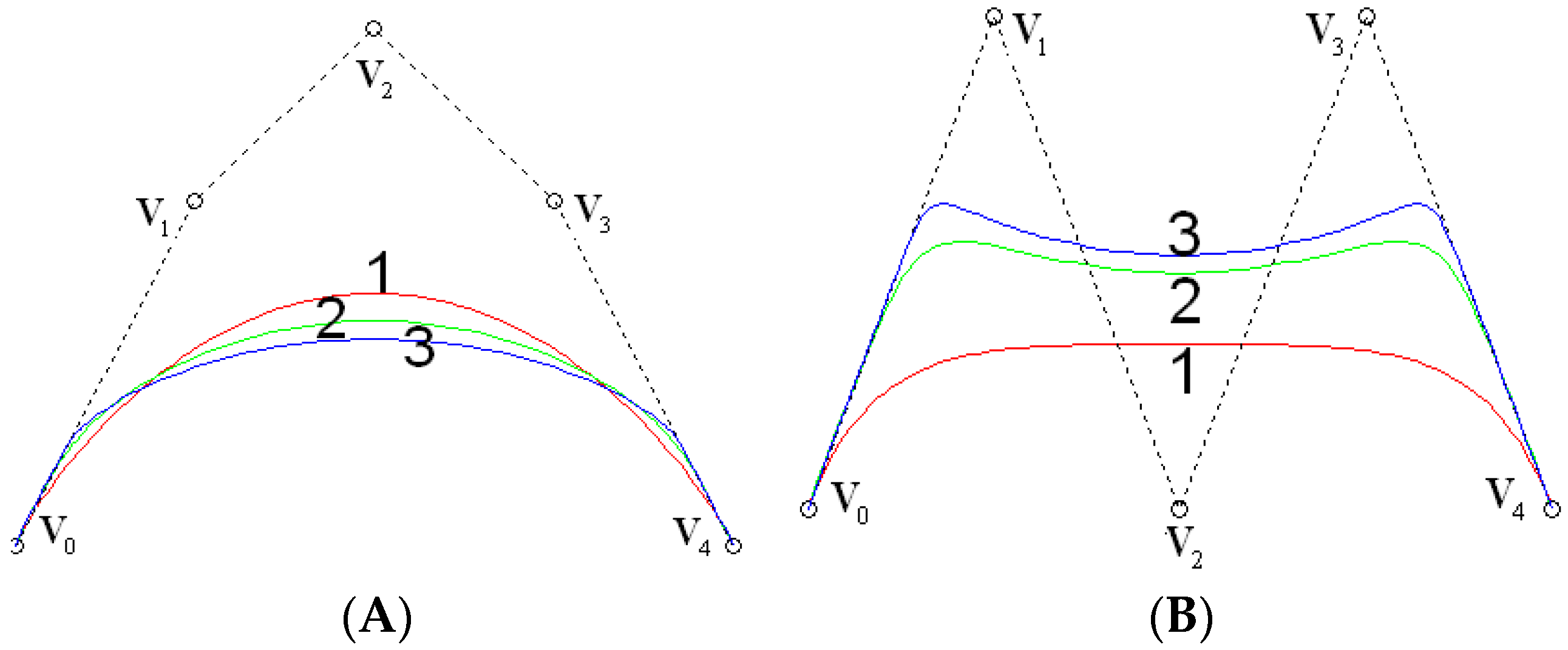
- (5)
- Shape adjustability property: Even if the control points of an adjustable Bézier curve are fixed, its shape can still be adjusted by changing the values of the three parameters , , and .
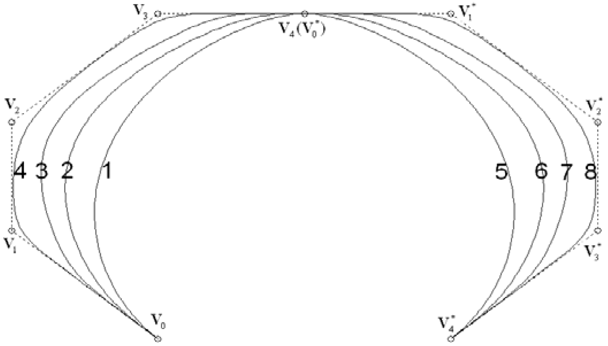
4. Composite Adjustable Bézier Curves
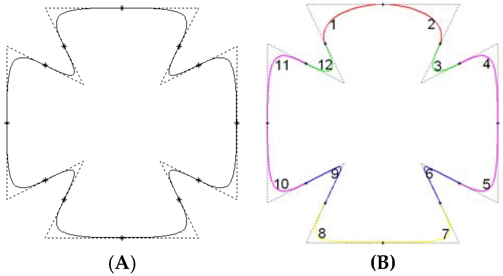
5. Adjustable Bézier Curves with Tangent Polygon
6. Conclusions
Conflicts of Interest
References
- Farin, G.; Hoschek, J.; Kim, M. Handbook of Comuter Aided Geometric Design; Elsevier: Amsterdam, The Netherlands, 2002. [Google Scholar]
- Wang, W.; Wang, G. Bézier curves with shape parameter. J. Zhejiang Univ. Sci. 2005, A6, 497–501. [Google Scholar] [CrossRef]
- Han, X.; Ma, Y.; Huang, X. A novel generalization of Bézier curve and surface. J. Comput. Appl. Math. 2008, 217, 180–193. [Google Scholar] [CrossRef]
- Yang, L.; Zeng, X. Bézier curves and surfaces with shape parameters. Int. J. Comput. Math. 2009, 86, 1253–1263. [Google Scholar] [CrossRef]
- Yan, L.; Liang, J. An extension of the Bézier model. Appl. Math. Comput. 2011, 218, 2863–2879. [Google Scholar] [CrossRef]
- Qin, X.; Hu, G.; Zhang, N.; Shen, X.; Yang, Y. A novel extension to the polynomial basis functions describing Bézier curves and surfaces of degree n with multiple shape parameters. Appl. Math. Comput. 2013, 223, 1–16. [Google Scholar] [CrossRef]
- Yan, L.; Han, X. Bézier-like curve and B-spline-like curve of order two. J. Inf. Comput. Sci. 2013, 10, 5483–5503. [Google Scholar] [CrossRef]
- Han, L.; Chu, Y.; Qiu, Z. Generalized Bézier curves and surfaces based on Lupaº q-analogue of Bernstein operator. J. Comput. Appl. Math. 2014, 261, 352–363. [Google Scholar] [CrossRef]
- Chen, Q.; Wang, G. A class of Bézier-like curves. Comput. Aided Geom. Des. 2003, 20, 29–39. [Google Scholar] [CrossRef]
- Han, X. Cubic trigonometric polynomial curves with a shape parameter. Comput. Aided Geom. Des. 2004, 21, 535–548. [Google Scholar] [CrossRef]
- Han, X.; Ma, Y.; Huang, X. The cubic trigonometric Bézier curve with two shape parameters. Appl. Math. Lett. 2009, 22, 226–231. [Google Scholar] [CrossRef]
- Han, X.; Zhu, Y. Curve construction based on five trigonometric blending functions. BIT Numer. Math. 2012, 52, 953–979. [Google Scholar] [CrossRef]
- Shen, W.; Wang, G. A class of quasi Bézier curves based on hyperbolic polynomials. J. Zhejiang Univ. Sci. 2005, 6A, 116–123. [Google Scholar] [CrossRef]
- Ahn, Y.J.; Lee, B.; Park, Y.; Yoo, J. Constrained polynomial degree reduction in the L2-norm equals best weighted Euclidean approximation of Bezier coefficients. Comput. Aided Geom. Des. 2004, 21, 181–191. [Google Scholar] [CrossRef]
- Ait-Haddou, R.; Barton, M. Constrained multi-degree reduction with respect to Jacobi norms. Comput. Aided Geom. Des. 2016, 42, 23–30. [Google Scholar] [CrossRef]
- Barsky, B.A.; Derose, T.D. Geometric continuity of parametric curves three equivalent characterizations. IEEE Comput. Graph. Appl. 1989, 9, 60–69. [Google Scholar] [CrossRef]
- Shi, F. Computer Aided Geometric Design and Non-Uniform Rational B-Spline; Higher Education Press: Beijing, China, 2013. (In Chinese) [Google Scholar]
- Yan, L.; Liang, J. A class of Algebraic-trigonometric blended splines. J. Comput. Appl. Math. 2011, 235, 1713–1729. [Google Scholar] [CrossRef]
- Hering, L. Closed (C2-and C3-continuous) Bézier and B-spline curves with given tangent polygons. Comput. Aided Des. 1983, 15, 3–6. [Google Scholar] [CrossRef]
- Fang, K. Closed (G2-continuous) Bézier curve with given tangent polygon. Chin. J. Numer. Math. 1991, 13, 34–38. [Google Scholar]


© 2016 by the author; licensee MDPI, Basel, Switzerland. This article is an open access article distributed under the terms and conditions of the Creative Commons Attribution (CC-BY) license (http://creativecommons.org/licenses/by/4.0/).
Share and Cite
Yan, L. Adjustable Bézier Curves with Simple Geometric Continuity Conditions. Math. Comput. Appl. 2016, 21, 44. https://doi.org/10.3390/mca21040044
Yan L. Adjustable Bézier Curves with Simple Geometric Continuity Conditions. Mathematical and Computational Applications. 2016; 21(4):44. https://doi.org/10.3390/mca21040044
Chicago/Turabian StyleYan, Lanlan. 2016. "Adjustable Bézier Curves with Simple Geometric Continuity Conditions" Mathematical and Computational Applications 21, no. 4: 44. https://doi.org/10.3390/mca21040044
APA StyleYan, L. (2016). Adjustable Bézier Curves with Simple Geometric Continuity Conditions. Mathematical and Computational Applications, 21(4), 44. https://doi.org/10.3390/mca21040044