Modeling Sound Propagation Using the Corrective Smoothed Particle Method with an Acoustic Boundary Treatment Technique

Abstract

The development of computational acoustics allows the simulation of sound generation and propagation in a complex environment. In particular, meshfree methods are widely used to solve acoustics problems through arbitrarily distributed field points and approximation smoothness flexibility. As a Lagrangian meshfree method, the smoothed particle hydrodynamics (SPH) method reduces the difficulty in solving problems with deformable boundaries, complex topologies, or multiphase medium. The traditional SPH method has been applied in acoustic simulation. This study presents the corrective smoothed particle method (CSPM), which is a combination of the SPH kernel estimate and Taylor series expansion. The CSPM is introduced as a Lagrangian approach to improve the accuracy when solving acoustic wave equations in the time domain. Moreover, a boundary treatment technique based on the hybrid meshfree and finite difference time domain (FDTD) method is proposed, to represent different acoustic boundaries with particles. To model sound propagation in pipes with different boundaries, soft, rigid, and absorbing boundary conditions are built with this technique. Numerical results show that the CSPM algorithm is consistent and demonstrates convergence with exact solutions. The main computational parameters are discussed, and different boundary conditions are validated as being effective for benchmark problems in computational acoustics.

1. Introduction

Numerical methods have been applied to model acoustic phenomena, and the development of computational acoustics allows the simulation of sound generation and propagation in a complex environment. Many classic numerical methods such as the finite difference method (FDM) [1], the finite element method (FEM) [2], the boundary element method (BEM) [3], and other modified methods [4,5], have been applied in spectral or temporal acoustic simulations. In particular, meshfree methods are widely applied to solve acoustics problems, because field points used in this method are arbitrarily distributed and the approximation smoothness order is chosen with flexibility. The method of fundamental solutions (MFS) [6], the multiple-scale reproducing kernel particle method (RKPM) [7], the element-free Galerkin method (EFGM) [8], and meshfree methods [9,10,11,12] are used to address certain acoustic problems, mainly in the frequency domain, and other methods like the equivalent source method (ESM) [13,14,15] solve problems in the time domain. Moreover, there is also a kind of method based on the fundamental solutions to realize the meshfree property, such as the singular boundary method [16,17,18].

The smoothed particle hydrodynamics (SPH) method, as a Lagrangian, meshfree particle method, was independently pioneered by Lucy [19] and Gingold and Monaghan [20], for solving astrophysical problems. As a Lagrangian approach, the SPH method has several advantages over the standard grid-based numerical method: (i) the numerical error generated by computing the advection is eliminated, since the advection term is included in the Lagrangian derivative; (ii) complicated domain topologies and moving boundaries are easily represented due to its Lagrangian property, as illustrated in recent reviews by Liu and Liu [21], Springel [22], and Monaghan [23]; (iii) the interface between different mediums can be naturally traced through the particle density, instead of using a special algorithm such as the volume-of-fluid; (iv) it is easy to implement and has a parallel processing ability, for the approximation is implemented in the local support domain instead of the whole computational domain [24,25]. Introducing the SPH method to acoustic computation can bring these advantages to this field.

Recently, the SPH method has been gradually used in acoustic computation, and some researchers have attempted to obtain the acoustic field through direct numerical simulation. Wolfe [26] simulated room reverberation with sound generation and reception, based on a SPH fluid mechanics algorithm, and Hahn [27] solved the fluid dynamic equations to obtain pressure perturbations during sound propagation. Both of these works can be seen as direct numerical simulations (DNS), based on the SPH method. However, for various acoustic waves in engineering problems, acoustic variables such as the variation in pressure, density, and velocity, are generally small. On the contrary, the values of pressure, density, and velocity exist on a much larger scale than any variation in these variables [28]. Acoustic wave equations are obtained based on the acoustic variables, to avoid solving fluid dynamic variables. Consequently, solving acoustic wave equations requires a lower computational burden compared to solving the fluid dynamic equations directly, and this approach is widely used in modeling engineering problems.

In our recent work, we proposed the use of the SPH method to solve acoustic wave equations, and tests on the sound propagation and interference simulation were conducted [29,30]. Some computational parameters were also discussed [31,32]. Based on these tests, the SPH method accurately solved acoustic wave equations, and some parameters were investigated, but only the traditional SPH method was used.

With the advancement of the SPH method, the traditional SPH method is modified or improved to reduce numerical error. Chen et al. [33,34] proposed the corrective smoothed particle method (CSPM) on the basis of Taylor series expansion in 1999. The CSPM is effective in reducing numerical error both inside the computational domain and around the boundary, so it has been used in different fields [35,36]. Other notable modifications or corrections of the SPH method include the reproducing kernel particle method [37], the finite particle method (FPM) [38,39], moving least square particle hydrodynamics (MLSPH) [40,41], and modified smoothed particle hydrodynamics (MSPH) [42]. The present study focuses on using the CSPM to improve the simulation accuracy of the SPH method for solving acoustic wave equations.

The implementation of boundary conditions in the SPH method is not as straightforward as in the grid-based numerical models. Historically, this characteristic has been regarded as a weak point of the particle method [43,44]. Several approaches have been proposed to treat boundary conditions for computational fluid dynamics. Among them, it is feasible to use virtual particles [45] to implement the boundary conditions. These virtual particles are allocated on and outside the boundary, as shown in several related works [46,47]. So far, a limited implementation of acoustic boundaries has been observed, and the rigid acoustic boundary developed from the solid boundary in fluid dynamics is shown in [26,27,29,30,31,32]. The boundary treatment technique for different acoustic boundaries is important for acoustic numerical analysis by the Lagrangian meshfree method.

The present paper is organized as follows: In Section 2, the CSPM formulations are provided to solve the acoustic wave equations. In Section 3, a hybrid meshfree-FDTD (finite difference time domain) method is proposed for acoustic boundary treatment. In Section 4, a sound propagation model is used to validate the CSPM algorithm, and the effects of different computational parameters are discussed. In Section 5, soft, rigid, and absorbing boundaries are used to simulate sound reflection and transmission, and numerical results are compared with theoretical solutions.

2. CSPM Formulations for Sound Waves

2.1. Basic Concepts of SPH

The kernel approximation of a function f(r) at particle i used in the SPH method can be written as a summation of neighboring particles, as:

$$\langle f({\mathit{r}}_i)\rangle ={\displaystyle \sum _{j=1}^N\frac{m_j}{{\rho }_j}f({\mathit{r}}_j)W_{ij}}$$

(1)

where f is a function of the position vector r, W_ij = W(r_i − r_j, h), W is the smoothing kernel function, h is the smoothing length defining the influence area of the smoothing function, N indicates the number of particles in the support domain, m_j is the mass of particle j, and ρ_j is the density. In the SPH convention, the kernel approximation operator is marked by the angle bracket < >.

The particle approximation for the derivative can be described as:

$$\langle \nabla \cdot f(\mathit{r})\rangle =-{\displaystyle \sum _{j=1}^N\frac{m_j}{{\rho }_j}}f({\mathit{r}}_j)\cdot {\nabla }_i{W}_{ij}$$

(2)

The present paper uses the cubic spline kernel function as the smoothing function. The cubic spline kernel is a widely used smoothing function which was originally used by Monaghan and Lattanzio [48]:

$$W(r,h)={\alpha }_D\{\begin{array}{cc}1-\frac{3}{2}{q}^2+\frac{3}{4}{q}^3& 0\le q\le 1\\ \frac{1}{4}{(2-q)}^3& 1\le q\le 2\\ 0& q\ge 2\end{array}$$

(3)

where q = r/h; and in one-, two-, and three-dimensional space, α_D = 1/h, 15/(7πh²), and 3/(2πh³), respectively.

2.2. Acoustic Wave Equations in Lagrangian Form

In fluid dynamics, the governing equations for constructing SPH formulations are the laws of continuity, momentum, and state, which can be found in [49]. The Lagrangian form of the governing equations are:

$$\frac{\mathrm{D}\rho }{\mathrm{D}t}=-\rho \nabla \cdot \mathit{v}$$

(4)

$$\frac{\mathrm{D}\mathit{v}}{\mathrm{D}t}=-\frac{1}{\rho }\nabla P+\nu {\nabla }^2\mathit{v}+\mathit{F}+\mathit{g}$$

(5)

$$\frac{\mathrm{D}P}{\mathrm{D}t}=c_0^2\frac{\mathrm{D}\rho }{\mathrm{D}t}$$

(6)

where ρ is the fluid density, v is the flow velocity, P is the pressure, t is time, and c is the speed of sound.

For most common acoustical problems, two assumptions are always used to simplify the question. On one hand, the medium is lossless and at rest. On the other hand, a small departure from quiet conditions occurs. In this work, the medium for sound propagation and reflection is ideal fluid, and the process is adiabatic. In addition, the sound pressure δp, the density change of particle δρ, and the particle velocity v are supposedly small, which can be expressed as:

$$\{\begin{array}{cc}P=p_0+\delta p,& \left|\delta p\right|<<p_0\\ \rho ={\rho }_0+\delta \rho ,& \left|\delta \rho \right|<<{\rho }_0\\ \mathit{v}=0+\mathit{v},& \left|\mathit{v}\right|<<c_0\end{array}$$

(7)

When substituting these expressions into the continuity and momentum equations (Equations (4) and (5)), ignoring the viscosity and force, the equations are as follows:

$$\frac{\mathrm{D}({\rho }_0+\delta \rho )}{\mathrm{D}t}=-({\rho }_0+\delta \rho )\nabla \cdot \mathit{v}$$

(8)

$$\frac{\mathrm{D}\mathit{v}}{\mathrm{D}t}=-\frac{1}{({\rho }_0+\delta \rho )}\nabla (p_0+\delta p)$$

(9)

Considering that ρ₀ and p₀ remain the same during the computation, they can also be expressed as:

$$\frac{\mathrm{D}\delta \rho }{\mathrm{D}t}=-({\rho }_0+\delta \rho )\nabla \cdot \mathit{v}$$

(10)

$$\frac{\mathrm{D}\mathit{v}}{\mathrm{D}t}=-\frac{1}{({\rho }_0+\delta \rho )}\nabla \delta p$$

(11)

Ignoring small quantities of first order, the Lagrangian form of the continuity and momentum equations governing the sound waves can be written as:

$$\frac{\mathrm{D}\delta \rho }{\mathrm{D}t}=-{\rho }_0\nabla \cdot \mathit{v}$$

(12)

$$\frac{\mathrm{D}\mathit{v}}{\mathrm{D}t}=-\frac{1}{{\rho }_0}\nabla \delta p$$

(13)

The state equation for ideal gas is written as:

$$\frac{\mathrm{D}\delta p}{\mathrm{D}t}=c_0^2\frac{\mathrm{D}\delta \rho }{\mathrm{D}t}$$

(14)

2.3. CSPM Formulations for Acoustic Waves

2.3.1. Particle Approximation of the Continuity Equation

Applying the particle approximation equation (Equation (2)) to the continuity equation (Equation (10)) yields:

$$\frac{\mathrm{D}\delta {\rho }_i}{\mathrm{D}t}=-({\rho }_0+\delta {\rho }_i){\displaystyle \sum _{j=1}^N\frac{m_j}{({\rho }_0+\delta {\rho }_j)}{\mathit{v}}_j{\nabla }_i{W}_{ij}}$$

(15)

where the subscript i and j stand for the variables associated with particles i and j, respectively.

By adding the gradient of the unity [49], another SPH formulation of the continuity equation can be obtained, as:

$$\frac{\mathrm{D}\delta {\rho }_i}{\mathrm{D}t}=-({\rho }_0+\delta {\rho }_i){\displaystyle \sum _{j=1}^N\frac{m_j}{({\rho }_0+\delta {\rho }_j)}{\mathit{v}}_{ij}{\nabla }_i{W}_{ij}}$$

(16)

where v_ij = v_i − v_j. Considering Equation (7), the continuity equation can also be written as:

$$\frac{\mathrm{D}\delta {\rho }_i}{\mathrm{D}t}=-{\displaystyle \sum _{j=1}^N{m}_j{\mathit{v}}_{ij}{\nabla }_i{W}_{ij}}$$

(17)

2.3.2. Particle Approximation of the Momentum Equation

When applying the particle approximation equation (Equation (2)) to the momentum equation (Equation (11)), it appears as:

$$\frac{\mathrm{D}{\mathit{v}}_i}{\mathrm{D}t}=-\frac{1}{({\rho }_0+\delta {\rho }_i)}{\displaystyle \sum _{j=1}^N\frac{m_j}{({\rho }_0+\delta {\rho }_j)}\delta p_j{\nabla }_i{W}_{ij}}$$

(18)

Other forms of the momentum equation can be written as:

$$\frac{\mathrm{D}{\mathit{v}}_i}{\mathrm{D}t}=-{\displaystyle \sum _{j=1}^N{m}_j\frac{\delta p_i+\delta p_j}{({\rho }_0+\delta {\rho }_i)({\rho }_0+\delta {\rho }_j)}{\nabla }_i{W}_{ij}}$$

(19)

$$\frac{\mathrm{D}{\mathit{v}}_i}{\mathrm{D}t}=-{\displaystyle \sum _{j=1}^N{m}_j\left[\frac{\delta p_i}{{({\rho }_0+\delta {\rho }_i)}^2}+\frac{\delta p_j}{{({\rho }_0+\delta {\rho }_j)}^2}\right]{\nabla }_i{W}_{ij}}$$

(20)

2.3.3. Particle Approximation of the Equation of State

Particle approximation of the equation of state for ideal gas is:

$$\frac{\mathrm{D}\delta p_i}{\mathrm{D}t}=c_0^2\frac{\mathrm{D}\delta {\rho }_i}{\mathrm{D}t}$$

(21)

2.3.4. Corrective Smoothed Particle Method

The Taylor series expansion is used to improve the accuracy of the SPH method, which is known as CSPM. If a function f(r) is assumed to be sufficiently smooth in a domain that contains r, the Taylor series expansion for f(r) in the vicinity of ξ can be written as:

$$f(\mathit{r})=f(\mathit{\xi })+({\mathit{r}}^{\alpha }-{\mathit{\xi }}^{\alpha })f_{\alpha }(\mathit{\xi })+\frac{1}{2!}({\mathit{r}}^{\alpha }-{\mathit{\xi }}^{\alpha })({\mathit{r}}^{\beta }-{\mathit{\xi }}^{\beta })f_{\alpha \beta }(\mathit{\xi })+\dots$$

(22)

where α, β = 1, 2, 3, represent different dimensional space and:

$$f_{\alpha }(\mathit{\xi })=\frac{\partial f(\mathit{\xi })}{\partial {\mathit{r}}^{\alpha }}$$

(23)

$$f_{\alpha \beta }(\mathit{\xi })=\frac{{\partial }^{2}f(\mathit{\xi })}{\partial {\mathit{r}}^{\alpha }\partial {\mathit{r}}^{\beta }}$$

(24)

Multiplying both sides of Equation (22) by a smoothing function W, defined in the local support domain Ω of ξ, and integrating over the support domain, the following formulation can be obtained:

$$\begin{array}{cc}{\displaystyle \underset{\mathsf{\Omega }}{\int }f(\mathit{r})W(\mathit{r}-\mathit{\xi },h)\mathrm{d}\mathit{r}}& ={\displaystyle \underset{\mathsf{\Omega }}{\int }f(\mathit{\xi })W(\mathit{r}-\mathit{\xi },h)\mathrm{d}\mathit{r}}+{\displaystyle \underset{\mathsf{\Omega }}{\int }({\mathit{r}}^{\alpha }-{\mathit{\xi }}^{\alpha })f_{\alpha }(\mathit{\xi })W(\mathit{r}-\mathit{\xi },h)\mathrm{d}\mathit{r}}\hfill \\ & +{\displaystyle \underset{\mathsf{\Omega }}{\int }\frac{1}{2!}({\mathit{r}}^{\alpha }-{\mathit{\xi }}^{\alpha })({\mathit{r}}^{\beta }-{\mathit{\xi }}^{\beta })f_{\alpha \beta }(\mathit{\xi })W(\mathit{r}-\mathit{\xi },h)\mathrm{d}\mathit{r}}+\dots \hfill \end{array}$$

(25)

From the above equation, a corrective kernel approximation for function f(r) at ξ can be written as:

$$\langle f(\mathit{\xi })\rangle =\frac{{\displaystyle \underset{\mathsf{\Omega }}{\int }f(\mathit{r})W(\mathit{r}-\mathit{\xi },h)\mathrm{d}\mathit{r}}}{{\displaystyle \underset{\mathsf{\Omega }}{\int }W(\mathit{r}-\mathit{\xi },h)\mathrm{d}\mathit{r}}}$$

(26)

Replacing W(r − ξ, h) with $\nabla$W(r − ξ, h), a corrective kernel approximation for the first derivative of f(r) at ξ can be written as:

$$\langle f_{\alpha }(\mathit{\xi })\rangle =\frac{{\displaystyle \underset{\mathsf{\Omega }}{\int }\left[f(\mathit{r})-f(\mathit{\xi })\right]\nabla W(\mathit{r}-\mathit{\xi },h)\mathrm{d}\mathit{r}}}{{\displaystyle \underset{\mathsf{\Omega }}{\int }({\mathit{r}}^{\alpha }-{\mathit{\xi }}^{\alpha })\nabla W(\mathit{r}-\mathit{\xi },h)\mathrm{d}\mathit{r}}}$$

(27)

The particle formulations of Equations (26) and (27) are given as:

$$f({\mathit{r}}_i)=\frac{{\displaystyle \sum _{j=1}^N\frac{m_j}{{\rho }_j}f({\mathit{r}}_j)W_{ij}}}{{\displaystyle \sum _{j=1}^N\frac{m_j}{{\rho }_j}{W}_{ij}}}$$

(28)

$$f_{\alpha }({\mathit{r}}_i)=\frac{{\displaystyle \sum _{j=1}^N\frac{m_j}{{\rho }_j}\left[f({\mathit{r}}_j)-f({\mathit{r}}_i)\right]{\nabla }_i{W}_{ij}}}{{\displaystyle \sum _{j=1}^N\frac{m_j}{{\rho }_j}({\mathit{r}}_j^{\alpha }-{\mathit{r}}_i^{\alpha }){\nabla }_i{W}_{ij}}}$$

(29)

The second order leap-frog integration [50] is used in this paper to update the parameters, and an all-pair searching approach [49] is used to realize the neighbour particle searching. The code is developed from the SPH algorithm used in [51].

3. Hybrid Meshfree-FDTD Method for Boundary Treatment

The meshfree method suffers from the problem that not enough particles in the support domain can be used for computation at the boundary. In the present paper, the FDTD method is introduced and is combined with the virtual particle technique, and thus, a technique based on the meshfree-FDTD hybrid method for acoustic boundary treatment is accordingly constructed. The feasibility and validity of the meshfree-FDTD hybrid method is verified by simulating sound propagation in pipes with boundaries.

Since the FDTD method was proposed by Yee [52] in 1966, it has received wide recognition and has been used to solve problems in many different research fields. The FDTD method can solve fundamental equations in the time domain. In this paper, for building the hybrid method, the FDTD method proposed by Wang [53], which was used to simulate an underwater acoustic boundary and the virtual particle technique, are combined.

In the hybrid meshfree-FDTD boundary treatment, three types of particles need to be built before computation, namely the fluid particle, the boundary particle, and the virtual particle. During the computation, the numerical methods chosen for these three kinds of particles are shown below.

$$\begin{array}{c}\mathrm{boundary}\mathrm{treatment}\\ \mathrm{for}\mathrm{particle}i\end{array}=\{\begin{array}{cc}\mathrm{meshfree}\mathrm{method}(\mathrm{SPH}/\mathrm{CSPM})& \mathrm{if}i=\mathrm{fluid}\mathrm{particles}\\ \mathrm{meshfree}\mathrm{method}(\mathrm{SPH}/\mathrm{CSPM})& \mathrm{if}i=\mathrm{boundary}\mathrm{particles}\\ \mathrm{FDTD}\mathrm{method}& \mathrm{if}i=\mathrm{virtual}\mathrm{particles}\end{array}$$

The hybrid meshfree-FDTD boundary treatment technique uses the meshfree method to obtain the parameter value of fluid and boundary particles, and the FDTD method to solve the parameter value of virtual particles.

Figure 1 is the sketch of the treatment of particles on a wall boundary when using the meshfree-FDTD method. The number of particles is represented by i. Virtual particles can be obtained through extending boundary particles to the outside of the computation region, and the distribution of virtual particles is parallel to the boundary particles, with equal particle spacing. The number of layers can be chosen according to the scale of the support domain. There should be enough virtual particles in the support domain for boundary particles, and virtual particles outside the support domain are unnecessary. In the present work, we use three layers of virtual particles to build the boundary.

For the soft boundary, the boundary conditions are:

$$\delta p=0$$

(30)

The formulation for the sound pressure of the virtual particles is written as:

$$\delta p_{i+1}=\delta p_{i+2}=\delta p_{i+3}=0$$

(31)

Assuming that the velocity perpendicular to the surface is u, the velocity of the virtual particles (e.g., particle i + 1) according to the central difference scheme should be calculated from the momentum equation as:

$$\frac{u_{i+1}^{(n)}-u_{i+1}^{(n-1)}}{\mathrm{\Delta }t}=-\frac{1}{{\rho }_0}\cdot \frac{(\delta p_{i+2}^{(n-1)}-\delta p_i^{(n-1)})}{2\mathrm{\Delta }x}$$

(32)

which can be written as:

$$u_{i+1}^{(n)}=u_{i+1}^{(n-1)}-\frac{(\delta p_{i+2}^{(n-1)}-\delta p_i^{(n-1)})\mathrm{\Delta }t}{2{\rho }_0\mathrm{\Delta }x}$$

(33)

where the superscript n represents the temporal index, ∆t is the time step, and ∆x is the particle spacing.

For the rigid boundary, the normal component of the pressure gradient on the surface equals zero when the wave is vertically incident with the boundary. Therefore, for the rigid case, the sound pressure δp satisfies the following:

$$\frac{\partial \delta p}{\partial \mathit{n}}=0,\delta \mathit{v}=0$$

(34)

where n represents the normal direction of the surface. According to the finite difference scheme, we have:

$$\frac{\delta p_{i+1}^{(n)}-\delta p_i^{(n)}}{\mathrm{\Delta }x}=0,\delta {\mathit{v}}_{i+1}^{(n)}=0$$

(35)

which can be written as:

$$\delta p_{i+1}^{(n)}=\delta p_i^{(n)},\delta {\mathit{v}}_{i+1}^{(n)}=0$$

(36)

For the absorbing boundary condition, the popular first-order absorbing boundary condition (ABC) proposed by Mur is used in the present work. Assuming that the ABC is located at x = x_i, sound propagates from the left side to the right side. The ABC can be written as:

$${\left[\frac{\partial f}{\partial x}-\frac{1}{c_0}\frac{\partial f}{\partial t}\right]}_{x=x_i}=0$$

(37)

where the field parameter f can be δp, u_x, or u_y in this equation. This leads to a different expression for virtual particles than that used in the meshfree-FDTD hybrid method, as follows:

$$f_{i+1}^{(n)}=f_i^{(n-1)}+\frac{c_0\mathrm{\Delta }t-\mathrm{\Delta }x}{c_0\mathrm{\Delta }t+\mathrm{\Delta }x}(f_i^{(n)}-f_{i+1}^{(n-1)})$$

(38)

The field parameter f in this equation can be δp or v.

4. Sound Propagation Simulation with CSPM

4.1. Sound Propagation Model

Sound propagation along ducts with different boundaries are discussed, as shown in Figure 2. In this model, sound propagates from x < 0 m to x ≥ 0 m, and the positive direction of the x-axis denotes the direction of sound propagation. The CSPM computational region is from −50 m to 150 m, and the propagation time is 0.25 s.

The sound pressure of the acoustic wave [54] in the ducts is written as:

$$\delta p(t,x)=2k^2\left[3+2\cos (kx-\omega t)\right]\exp \left[\frac{-\ln 2}{200}{(kx-\omega t)}^2\right]$$

(39)

where t denotes time, x is the geometric position in the propagation direction, ω is the angular frequency of the sound wave, and k = ω/c₀ is the wave number. In addition, the sound speed c₀ = 340 m/s, and ω = 340 rad/s.

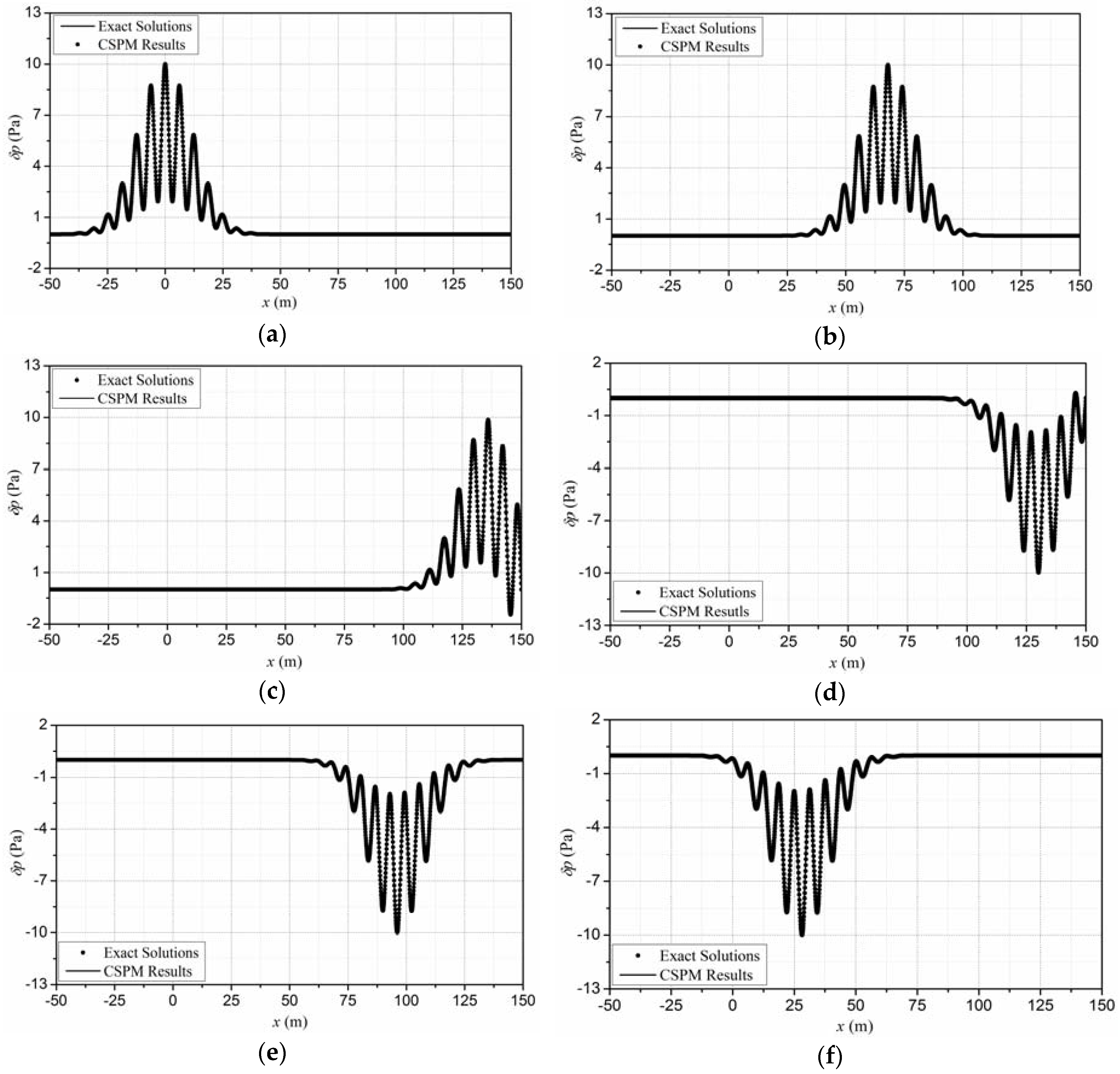
4.2. Verification of the Meshfree Algorithm

Table 1. Parameters for the corrective smoothed particle method (CSPM) algorithm for sound propagation modeling.

Computational Parameters	Values
∆x	0.04 m
h	0.058 m
Kernel Type	Cubic Spline
CCFL	0.10
c0	340 m/s
ρ0	1.0 kg/m3

lists the computational parameters that are used in the CSPM algorithm for sound propagation. The Courant-Friedriches-Lewy number is written as C_CFL for short, and C_CFL = u∆t/∆x.

In order to verify the algorithm, the CSPM algorithm is built to solve acoustic wave equations for sound propagation modeling. The costing central processing unit (CPU) time for the CSPM is 55.6 s, with the performance of computation measured on the Intel Core i3-3240 with RAM 4.00 GB (Gigabyte Technology Co., Ltd., New Taipei City, Taiwan). Then, the simulation results are compared to theoretical solutions, as shown in Figure 3. In this figure, solid lines demonstrate theoretical solutions, and points represent the CSPM simulation results. For clearly identifying different points, they are plotted at intervals of 14 grid points.

From the figure, it can be seen that several peaks and valleys appear in the graph between −50 m and 150 m. The algorithm is able to model the sound propagation process, and the CSPM simulation results are in good agreement with the theoretical solutions.

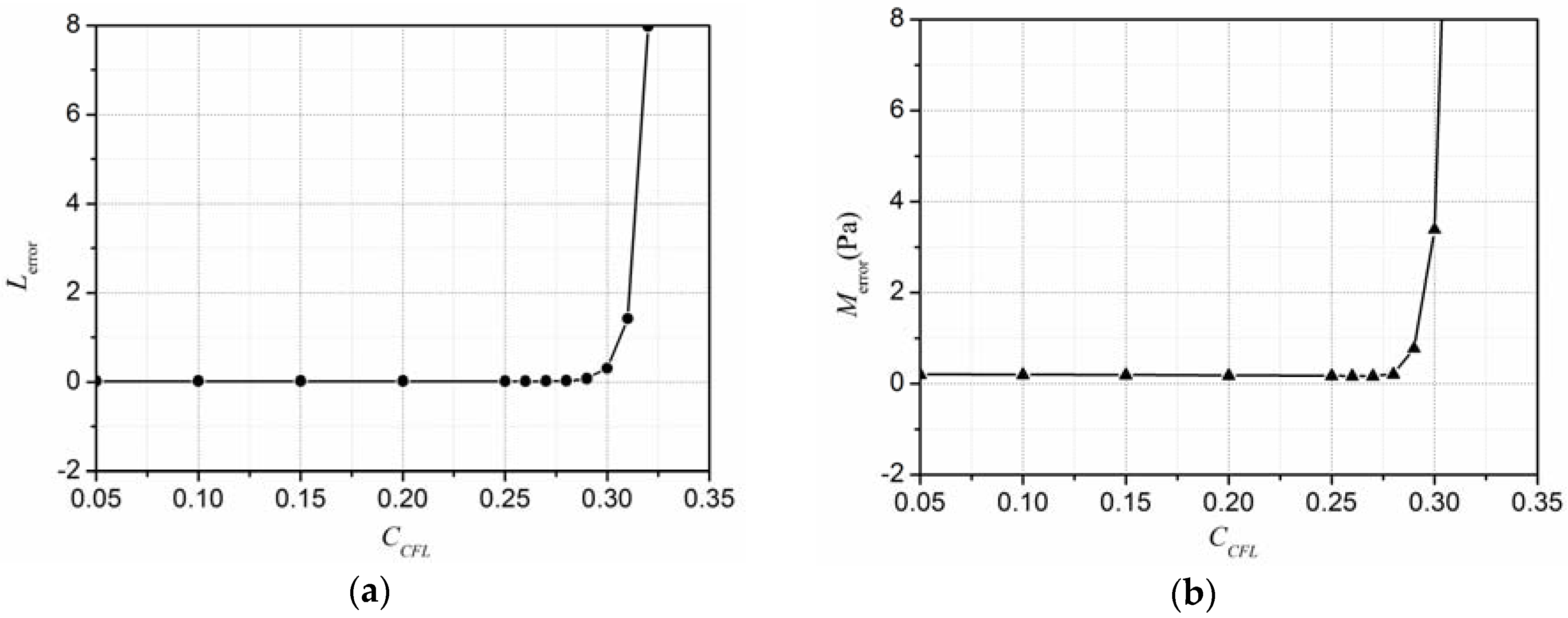
4.3. Discussion on Computational Parameters

In this section, the effects of the initial particle spacing and the time step on the accuracy of the present CSPM method is discussed. The method is compared with theoretical solutions. The numerical accuracy is evaluated with the relative root mean square errors (L_error) and the maximum error (M_error), which are given as follows:

$$L_{\mathrm{error}}\left(\delta p\right)=\frac{\sqrt{\frac{1}{N}{\displaystyle \sum _{i=1}^N{\left|\delta p\left(i\right)-\delta \overline{p}\left(i\right)\right|}^2}}}{\sqrt{\frac{1}{N}{\displaystyle \sum _{i=1}^N{\left|\delta \overline{p}\left(i\right)\right|}^2}}}$$

(40)

$$M_{\mathrm{error}}\left(\delta p\right)=\underset{1\le i\le N}{\max }\left|\delta p\left(i\right)-\delta \overline{p}\left(i\right)\right|$$

(41)

where $\delta p(i)$ and $\delta \overline{p}(i)$ are simulation results and theoretical solutions at particle i, and N is the total number of particles in the computation domain.

The convergence rate (R_error) for L_error and M_error are evaluated as:

$$R_{\mathrm{error}}=\left|\frac{\ln \left[Error(N{P}_{\max })\right]-\ln \left[Error(N{P}_{\min })\right]}{\ln \left(N{P}_{\max }\right)-\ln \left(N{P}_{\min }\right)}\right|$$

(42)

where Error represents L_error or M_error, and NP_max and NP_min represent the maximum and minimum number of particles in the computational domain, respectively.

Sound propagation with particle spacing changing from 0.02 to 0.10 m is computed. Then, the CSPM numerical error of the sound pressure according to Equations (40) and (41), is shown in Figure 4. In the computation, the ratio of the particle spacing to the smoothing length remains the same.

From the figure, it can be seen that, when the particle spacing increases, L_error and M_error increase gradually. L_error and M_error are the smallest at particle spacing ∆x = 0.02 m, which are 1.5 × 10⁻³ and 0.047 Pa, respectively. When at particle spacing ∆x = 0.10 m, L_error and M_error reach 0.126 and 1.17 Pa, respectively. The convergence rate for L_error and M_error is about 1.997 and 1.998, respectively, and 1.998 on average. In conclusion, the CSPM algorithm shows a good convergence in the simulation of sound propagation.

Similarly, the numerical error of sound propagation by using the CSPM algorithms a with different C_CFL is also discussed. When the C_CFL changes from 0.05 to 0.32, L_error and M_error are computed, as shown in Figure 5.

As can be seen from the figure, in the region of 0.05 ≤ C_CFL ≤ 0.28, with the increasing of C_CFL, L_error and M_error increase slowly. When C_CFL is equal to 0.05, L_error and M_error are 0.02 and 0.19 Pa, respectively. When C_CFL is 0.28, L_error and M_error are 0.03 and 0.20 Pa, respectively. Moreover, when C_CFL is greater than 0.28, L_error and M_error increase sharply with increased C_CFL. In general, according to the present case, for maintaining computational accuracy and efficiency in the numerical simulation, C_CFL is preferably set as under 0.28.

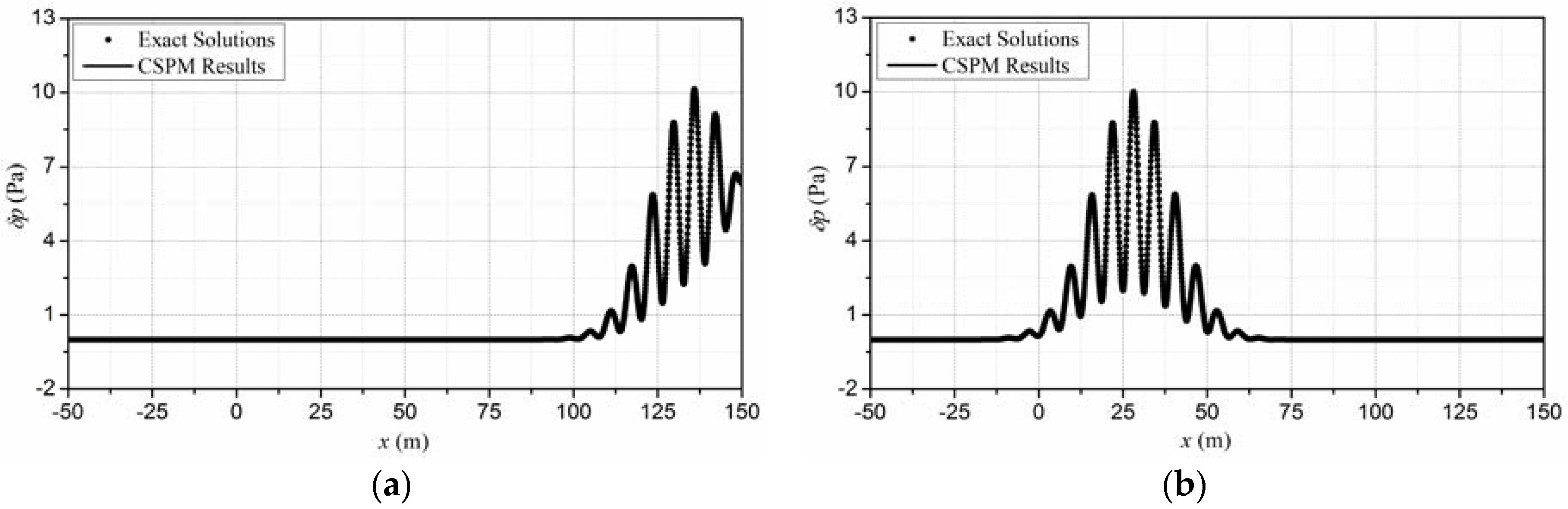
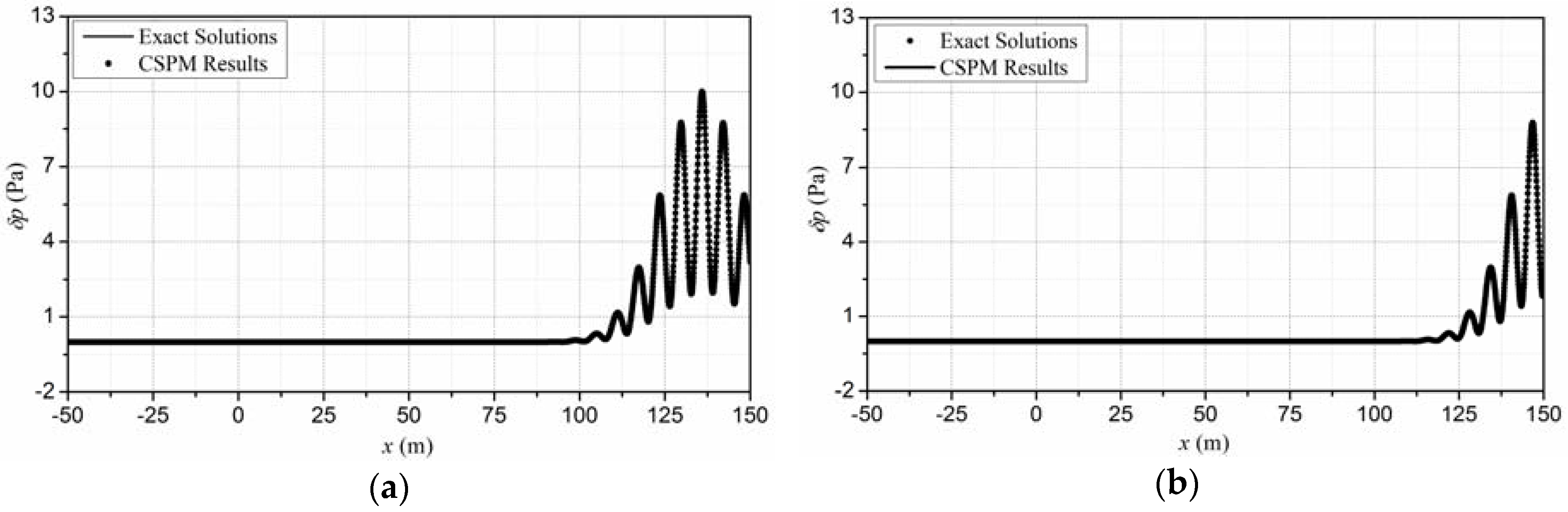
5. Application of Different Acoustic Boundaries

5.1. Soft Boundary

The sound propagation model with a soft boundary is built to validate the boundary treatment technique. The computational domain is −10 m ≤ x ≤ 190 m, and the computational parameters are shown in Table 1. The soft boundary is located at x = 150 m. Then, the sound pressure at t = 0 s, 0.20 s, 0.40 s, 0.50 s, 0.60 s, and 0.80 s is computed, and the simulation results are shown in Figure 6.

Figure 6a shows the sound pressure at the initial time. Figure 6b is the sound pressure at t = 0.20 s, where the sound wave is propagating but has not reached the soft boundary. Figure 6c,d is the sound pressure at t = 0.40 s and 0.50 s, respectively. A reflected sound wave is generated by the soft boundary and it propagates along the −x direction. There is an overlap between the incident sound wave and reflected sound. At t = 0.60 s to 0.80 s, the reflected sound wave continues to propagate along the x direction, as shown in Figure 6e,f.

It can be seen from the figure that the CSPM results are in good agreement with the theoretical solutions, namely, the soft boundary can be accurately represented with the hybrid meshfree-FDTD acoustic boundary treatment technique.

5.2. Rigid Boundary

The sound reflection model with a rigid boundary at x = 150 m is built. Simulation results are compared to the theoretical solutions in Figure 7. Since the sound propagation process before reaching the boundary is the same as in the last section, Figure 7a and b only give the sound pressure of particles at t = 0.40 s and 0.80 s, respectively.

Figure 7 shows that the CSPM method predicts each peak of the sound waves to be almost the same as the theoretical solutions. The numerical simulation can correctly handle the process of sound propagation and reflection.

5.3. Absorbing Boundary

To model the sound propagation in an unbounded domain, the artificial boundary condition has to be used, to eliminate the reflection from the edges of the computation domain. The sound propagation model with the implementation of an absorbing boundary is built, and the absorbing boundary is located at x = 150 m. The simulation results are shown in Figure 8.

Unlike soft and rigid boundaries, under the effect of the absorbing boundary, the incident wave is absorbed with no reflected waves. It can be seen from the figure that the CSPM simulation results are in good agreement with the theoretical solutions at each time point. There is almost no reflected sound pressure in the last figure. The absorbing boundary works well in the computation.

6. Conclusions

The Lagrangian meshfree-CSPM method is proposed, to improve the accuracy in solving acoustic wave equations, and different acoustic boundary conditions are implemented with a novel boundary treatment technique, based on the hybrid meshfree-FDTD method. The findings lead to the following conclusions:

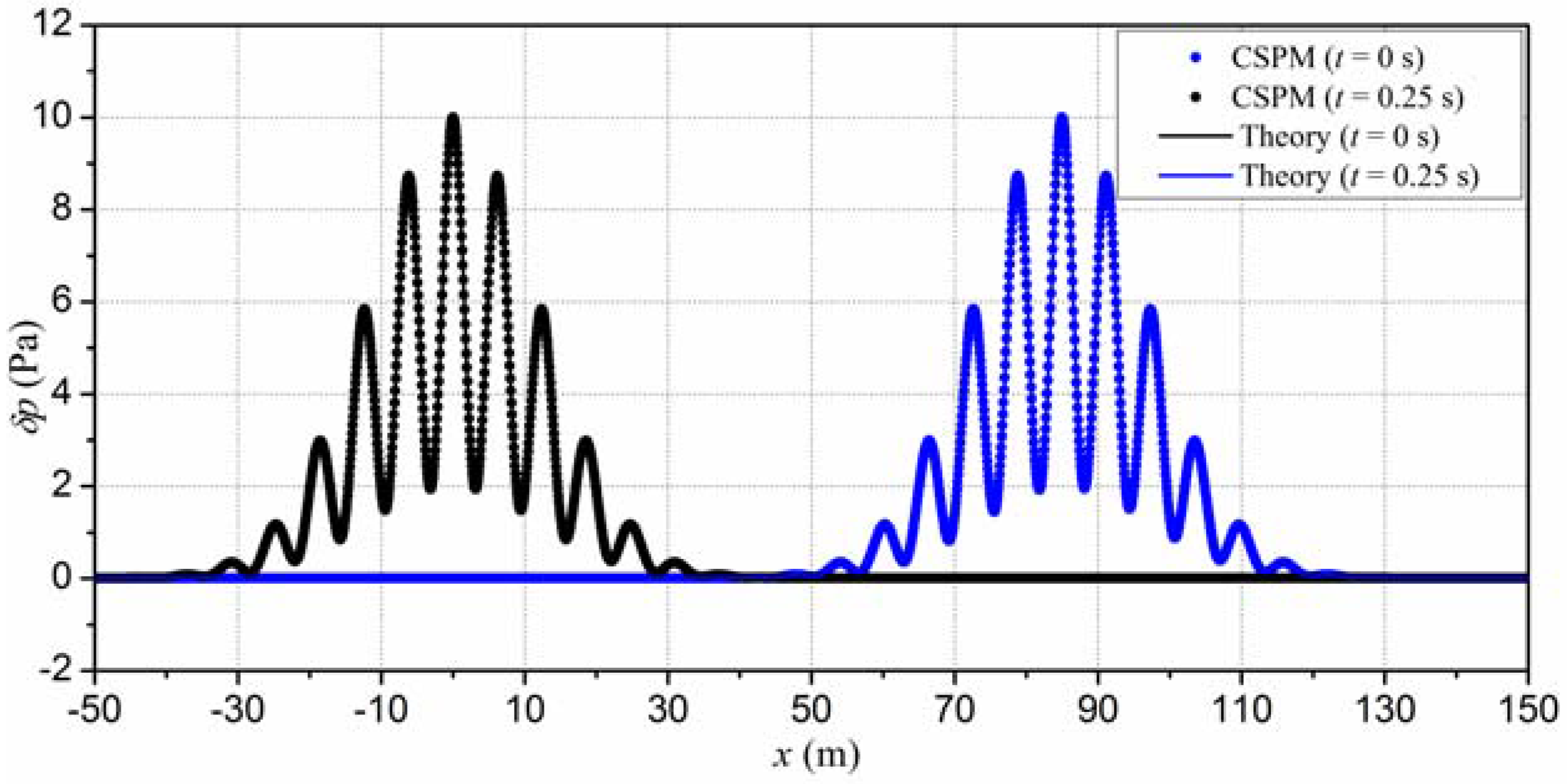
• The CSPM method is proposed to simulate sound propagation in the time domain by solving acoustic wave equations. Numerical results agree well with theoretical solutions in the modeling of sound propagation in pipes.
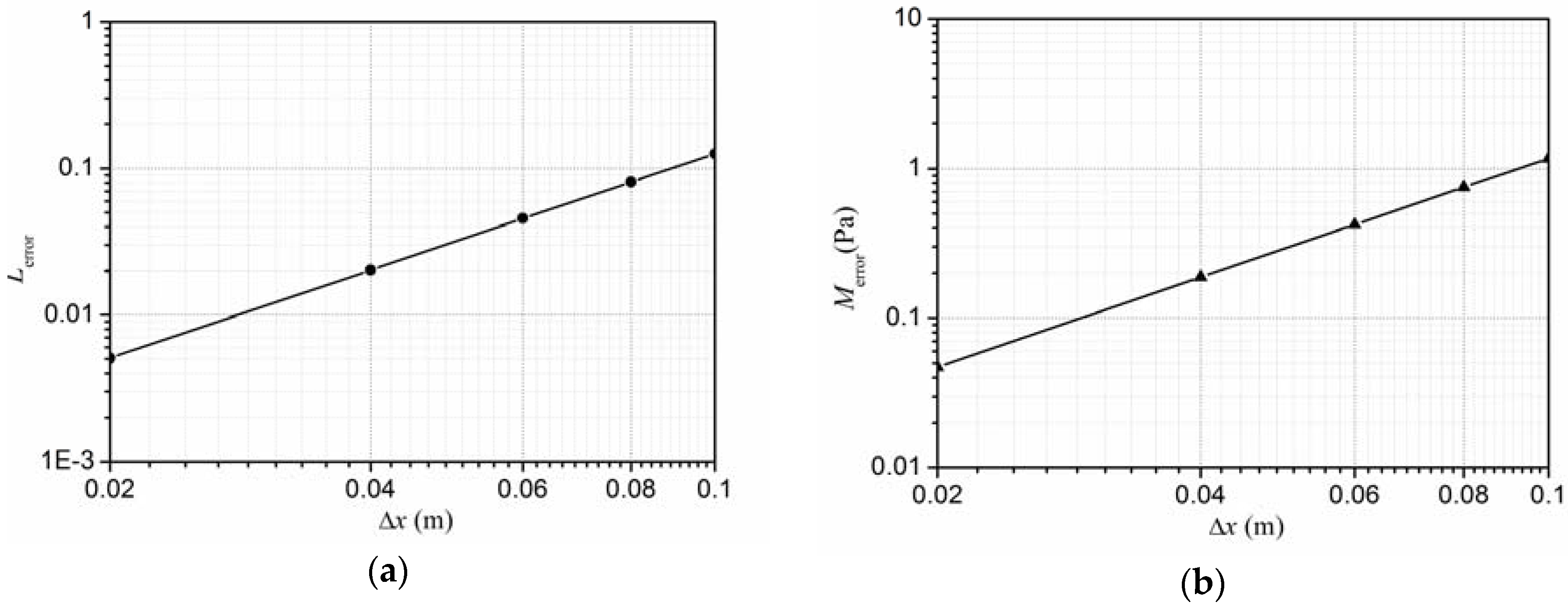
• The CSPM method exhibits good convergence, while maintaining a constant ratio of the particle spacing to the smoothing length. According to the present work, the convergence rate is about 1.998 and the CCFL is suggested to be under 0.28.
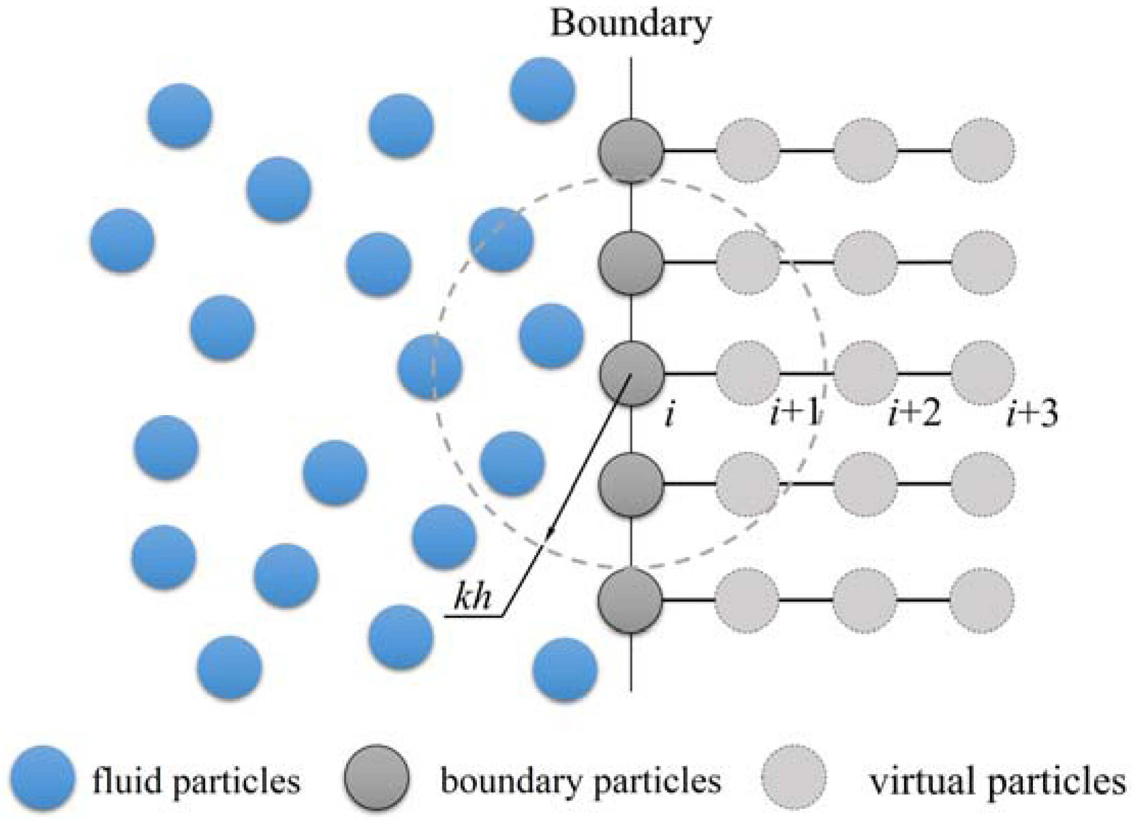
• A hybrid meshfree-FDTD method is developed and used as an acoustic boundary treatment technique for the meshfree method, and different boundaries are built for virtual particles by using this technique.
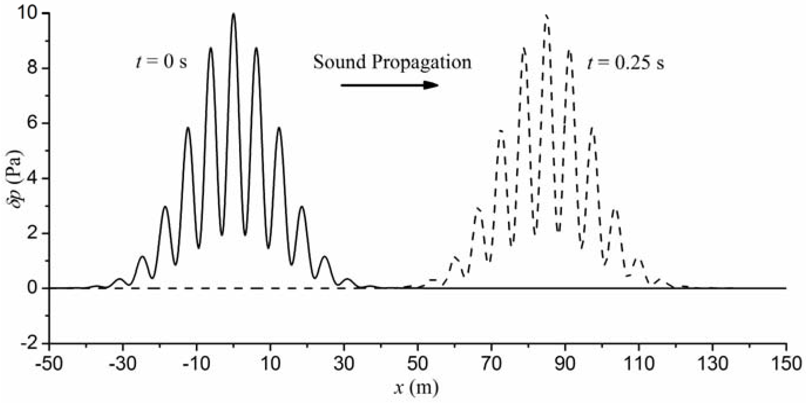
• The sound propagation and reflection computed with soft, rigid, and absorbing boundaries, agree well with theoretical solutions for modeling sound propagation.

References

1. Lee, D.; McDaniel, S.T. Ocean Acoustic Propagation by Finite Difference Methods; Pergamon Press: Oxford, UK, 2014. [Google Scholar]
2. Harari, I. A survey of finite element methods for time-harmonic acoustics. Comput. Methods Appl. Mech. Eng. 2006, 195, 1594–1607. [Google Scholar] [CrossRef]
3. Kythe, P.K. An Introduction to Boundary Element Methods; CRC Press: Boca Raton, FL, USA, 1995. [Google Scholar]
4. Li, W.; Chai, Y.B.; Lei, M.; Liu, G.R. Analysis of coupled structural-acoustic problems based on the smoothed finite element method (S-FEM). Eng. Anal. Bound. Elem. 2014, 42, 84–91. [Google Scholar] [CrossRef]
5. Tadeu, A.; Stanak, P.; Sladek, J.; Sladek, V. Coupled BEM-MLPG acoustic analysis for non-homogeneous media. Eng. Anal. Bound. Elem. 2014, 44, 161–169. [Google Scholar] [CrossRef]
6. Fairweather, G.; Karageorghis, A.; Martin, P.A. The method of fundamental solutions for scattering and radiation problems. Eng. Anal. Bound. Elem. 2003, 27, 759–769. [Google Scholar] [CrossRef]
7. Uras, R.A.; Chang, C.T.; Chen, Y.; Liu, W.K. Multiresolution reproducing kernel particle methods in acoustics. J. Comput. Acoust. 1997, 5, 71–94. [Google Scholar] [CrossRef]
8. Bouillard, P.; Suleau, S. Element-free Galerkin solutions for Helmholtz problems: Formulation and numerical assessment of the pollution effect. Comput. Methods Appl. Mech. Eng. 1998, 162, 317–335. [Google Scholar] [CrossRef]
9. Fu, Z.J.; Chen, W.; Gu, Y. Burton-Miller-type singular boundary method for acoustic radiation and scattering. J. Sound Vib. 2014, 333, 3776–3793. [Google Scholar] [CrossRef]
10. Chen, W.; Zhang, J.Y.; Fu, Z.J. Singular boundary method for modified Helmholtz equations. Eng. Anal. Bound. Elem. 2014, 44, 112–119. [Google Scholar] [CrossRef]
11. Godinho, L.; Amado-Mendes, P.; Carbajo, J.; Ramis-Soriano, J. 3D numerical modelling of acoustic horns using the method of fundamental solutions. Eng. Anal. Bound. Elem. 2015, 51, 64–73. [Google Scholar] [CrossRef]
12. Godinho, L.; Soares, D.; Santos, P.G. Efficient analysis of sound propagation in sonic crystals using an ACA–MFS approach. Eng. Anal. Bound. Elem. 2016, 69, 72–85. [Google Scholar] [CrossRef]
13. Lee, S. Review: The use of equivalent source method in computational acoustics. J. Comput. Acoust. 2016, 24, 1630001. [Google Scholar] [CrossRef]
14. Lee, S.; Brentner, K.S.; Morris, P.J. Assessment of time-domain equivalent source method for acoustic scattering. AIAA J. 2011, 49, 1897–1906. [Google Scholar] [CrossRef]
15. Lee, S.; Brentner, K.S.; Morris, P.J. Acoustic scattering in the time domain using an equivalent source method. AIAA J. 2010, 48, 2772–2780. [Google Scholar] [CrossRef]
16. Li, J.; Chen, W.; Fu, Z.; Sun, L. Explicit empirical formula evaluating original intensity factors of singular boundary method for potential and Helmholtz problems. Eng. Anal. Bound. Elem. 2016, 73, 161–169. [Google Scholar] [CrossRef]
17. Chen, W.; Li, J.; Fu, Z. Singular boundary method using time-dependent fundamental solution for scalar wave equations. Comput. Mech. 2016, 58, 717–730. [Google Scholar] [CrossRef]
18. Li, J.; Chen, W.; Fu, Z. Numerical investigation on convergence rate of singular boundary method. Math. Probl. Eng. 2016, 2016, 3564632. [Google Scholar] [CrossRef]
19. Lucy, L.B. A numerical approach to the testing of the fission hypothesis. Astron. J. 1977, 82, 1013–1024. [Google Scholar] [CrossRef]
20. Gingold, R.A.; Monaghan, J.J. Smoothed Particle Hydrodynamics-theory and application to non-spherical stars. Mon. Not. R. Astron. Soc. 1977, 181, 375–389. [Google Scholar] [CrossRef]
21. Liu, M.B.; Liu, G.R.; Zong, Z. An overview on smoothed particle hydrodynamics. Int. J. Comput. Methods 2008, 5, 135–188. [Google Scholar] [CrossRef]
22. Springel, V. Smoothed particle hydrodynamics in astrophysics. Annu. Rev. Astron. Astrophys. 2010, 48, 391–430. [Google Scholar] [CrossRef]
23. Monaghan, J.J. Smoothed particle hydrodynamics and its diverse applications. Annu. Rev. Fluid Mech. 2012, 44, 323–346. [Google Scholar] [CrossRef]
24. Liu, M.B.; Liu, G.R. Smoothed Particle Hydrodynamics (SPH): An overview and recent developments. Arch. Comput. Methods Eng. 2010, 17, 25–76. [Google Scholar] [CrossRef]
25. Fan, H.; Bergel, G.L.; Li, S. A hybrid peridynamics-SPH simulation of soil fragmentation by blast loads of buried explosive. Int. J. Impact Eng. 2016, 87, 14–27. [Google Scholar] [CrossRef]
26. Wolfe, C.T. Acoustic Modeling of Reverberation Using Smoothed Particle Hydrodynamics. Master’s Thesis, University of Colorado, Denver, CO, USA, 2007. [Google Scholar]
27. Hahn, P. On the Use of Meshfree Methods in Acoustic Simulations. Master’s Thesis, University of Wisconsin-Madison, Madison, WI, USA, 2009. [Google Scholar]
28. Bruneau, M. Chapter 1: Equations of Motion in Non-Dissipative Fluid. In Fundamentals of Acoustics; John Wiley & Sons: New York, NY, USA, 2010. [Google Scholar]
29. Zhang, Y.O.; Zhang, T.; Ouyang, H.; Li, T.Y. Smoothed particle hydrodynamics simulation of sound reflection and transmission. J. Acoust. Soc. Am. 2014, 136, 2224. [Google Scholar] [CrossRef]
30. Zhang, Y.O.; Zhang, T.; Ouyang, H.; Li, T.Y. SPH simulation of sound propagation and interference. In Proceedings of the 5th International Conference of Computational Method, Cambridge, UK, 28–30 July 2014.
31. Zhang, Y.O.; Zhang, T.; Ouyang, H.; Li, T.Y. Efficient SPH simulation of time-domain acoustic propagation. Eng. Anal. Bound. Elem. 2016, 62, 112–122. [Google Scholar] [CrossRef]
32. Zhang, Y.O.; Zhang, T.; Ouyang, H.; Li, T.Y. SPH simulation of acoustic waves: Effects of frequency, sound pressure, and particle spacing. Math. Probl. Eng. 2015, 348314. [Google Scholar] [CrossRef]
33. Chen, J.K.; Beraun, J.E.; Carney, T.C. A corrective smoothed particle method for boundary value problems in heat conduction. Int. J. Numer. Methods Eng. 1999, 46, 231–252. [Google Scholar] [CrossRef]
34. Chen, J.K.; Beraun, J.E.; Jih, C.J. Completeness of corrective smoothed particle method for linear elastodynamics. Comput. Mech. 1999, 24, 273–285. [Google Scholar] [CrossRef]
35. Chen, J.K.; Beraun, J.E.; Jih, C.J. An improvement for tensile instability in smoothed particle hydrodynamics. Comput. Mech. 1999, 23, 279–287. [Google Scholar] [CrossRef]
36. Chen, J.K.; Beraun, J.E.; Jih, C.J. A corrective smoothed particle method for transient elastoplastic dynamics. Comput. Mech. 2001, 27, 177–187. [Google Scholar] [CrossRef]
37. Liu, W.K.; Chen, Y. Wavelet and multiple scale reproducing kernel methods. Int. J. Numer. Methods Fluids 1995, 21, 901–931. [Google Scholar] [CrossRef]
38. Liu, M.B.; Liu, G.R. Restoring particle consistency in smoothed particle hydrodynamics. Appl. Numer. Math. 2006, 56, 19–36. [Google Scholar] [CrossRef]
39. Liu, M.B.; Xie, W.P.; Liu, G.R. Modeling incompressible flows using a finite particle method. Appl. Math. Model. 2005, 29, 1252–1270. [Google Scholar] [CrossRef]
40. Dilts, G.A. Moving-Least-Squares-particle hydrodynamics I: Consistency and stability. Int. J. Numer. Methods Eng. 1999, 44, 1115–1155. [Google Scholar] [CrossRef]
41. Dilts, G.A. Moving least square particle hydrodynamics II: Conservation and boundaries. Int. J. Numer. Methods Eng. 2000, 48, 1503–1524. [Google Scholar] [CrossRef]
42. Zhang, G.M.; Batra, R.C. Modified smoothed particle hydrodynamics method and its application to transient problems. Comput. Mech. 2004, 34, 137–146. [Google Scholar] [CrossRef]
43. Schussler, M.; Schmitt, D. Comments on smoothed particle hydrodynamics. Astron. Astrophys. 1981, 97, 373–379. [Google Scholar]
44. Agertz, O.; Moore, B.; Stadel, J.; Potter, D.; Miniati, F.; Read, J.; Mayer, L.; Gawryszczak, A.; Kravtosov, A.; Nordlund, A.; et al. Fundamental differences between SPH and grid methods. Mon. Not. R. Astron. Soc. 2007, 380, 963–978. [Google Scholar] [CrossRef]
45. Monaghan, J.J. Simulation free surface flows with SPH. J. Comput. Phys. 1994, 110, 399–406. [Google Scholar] [CrossRef]
46. Randles, P.W.; Libersky, L.D. Smoothed particle hydrodynamics: Some recent improvements and applications. Comput. Methods Appl. Mech. Eng. 1996, 138, 375–408. [Google Scholar] [CrossRef]
47. Liu, M.B.; Liu, G.R.; Lam, K.Y. Investigation into water mitigations using a meshfree particle method. Shock Waves 2002, 12, 181–195. [Google Scholar] [CrossRef]
48. Monaghan, J.J.; Lattanzio, J.C. A refined particle method for astrophysical problems. Astron. Astrophys. 1985, 149, 135–143. [Google Scholar]
49. Liu, G.R.; Liu, M.B. Chapter 1.4: Meshfree Particle Methods. In Smoothed Particle Hydrodynamics: A Meshfree Particle Method; World Scientific: Singapore, 2003. [Google Scholar]
50. Kelager, M. Lagrangian Fluid Dynamics Using Smoothed Particle Hydrodynamics; Technical Report; University of Copenhagen: Copenhagen, Denmark, 2006. [Google Scholar]
51. Li, X.; Zhang, T.; Zhang, Y.O. Time domain simulation of sound waves using smoothed particle hydrodynamics algorithm with artificial viscosity. Algorithms 2015, 8, 321–335. [Google Scholar] [CrossRef]
52. Yee, K.S. Numerical solution of initial boundary value problems involving Maxwell’s equations in isotropic media. IEEE Trans. Antennas Propag. 1966, 14, 302–307. [Google Scholar]
53. Wang, S. Finite-difference time-domain approach to underwater acoustic scattering problems. J. Acoust. Soc. Am. 1996, 99, 1924–1931. [Google Scholar] [CrossRef]
54. Li, K.; Huang, Q.B.; Wang, J.L.; Lin, L.G. An improved localized redial basis function meshfree method for computational aeroacoustics. Eng. Anal. Bound. Elem. 2011, 35, 47–55. [Google Scholar] [CrossRef]
Figure 1. The sketch of simulating the acoustic boundary using the hybrid meshfree-finite difference time domain (FDTD) method.
Mca 22 00026 g001
Figure 2. The model of sound propagation in a pipe along the x-axis.
Mca 22 00026 g002
Figure 3. Sound pressure computation between corrective smoothed particle method results and theoretical solutions.
Mca 22 00026 g003
Figure 4. Convergence curve for the CSPM method; (a) Lerror and (b) Merror.
Mca 22 00026 g004
Figure 5. Sound pressure error versus CCFL in the CSPM computation; (a) Lerror and (b) Merror.
Mca 22 00026 g005
Figure 6. Comparison between CSPM results and exact solutions with sound reflecting from the soft boundary: (a) t = 0 s; (b) t = 0.20 s; (c) t = 0.40 s; (d) t = 0.50 s; (e) t = 0.60 s and (f) t = 0.80 s.
Mca 22 00026 g006
Figure 7. Comparison between CSPM results and exact solutions with sound reflecting from the rigid boundary: (a) t = 0.40 s; (b) t = 0.80 s.
Mca 22 00026 g007
Figure 8. Comparison between CSPM results and exact solutions with sound propagation through absorbing boundary: (a) t = 0.40 s; (b) t = 0.45 s; (c) t = 0.50 s and (d) t = 0.60 s.
Mca 22 00026 g008aMca 22 00026 g008b