1. Introduction
In previous work, Bajo et al. [
1] investigated the optimal options hedging strategy for a firm, where the role of production risk and basis risk were taken into account. We provide a further extension by introducing futures as a plus instrument to hedge against price risk and background risk. In fact, the model of Bajo et al. is a special model of our proposed model. There are at least two features of this problem that suggest the need for extension. First, since the firm faces multiple sources of risk, a single hedging instrument cannot completely remove all of the income uncertainty. Possibly, such instruments are both futures and options, which have been proved suitable for hedging linear or nonlinear risk. Second, Frank et al. [
2] pointed out that background risk, additive risk or multiplicative, was prevailing, which could not be ignored. Examples of background risks include uncertain labor income, uncertainty about the terminal value of fixed assets and so on. These factors have a great influence on investment decisions.
After the seminal work of Sandmo [
3], a large body of research has been focused on the production theory of the competitive firm under price uncertainty. The commonly used approach is confined to choosing only futures for hedging risk, from which two celebrated theorems (separation theorem and full-hedging theorem) emanate, see e.g., [
4,
5,
6]).
The aforementioned studies discussed the establishment of the two theorems under different conditions. It is well-known that linear hedge instruments, such as futures or forwards, are suitable to be used for hedging with linear risk. However, it seems powerless in hedging with nonlinear risk. Nonlinear risk can be hedged using nonlinear instruments such as options, for instance. The conclusions were also supported by Darren [
7], Topaloglou et al. [
8] and Maciej [
9]. To fill the gap of using options as a hedging instrument, Machnes [
10] examined the behavior of a competitive firm in the presence of commodity options and price uncertainty. In fact, nonlinear risk is prevailing. For example, if state-dependent variables are considered in the model, it inevitably leads to nonlinear risk. Benninga and Oosterhof [
11] showed the role of options hedging under state-dependent preferences. Wong [
12] further examined the behavior of the competitive firm under output price uncertainty and state-dependent preferences by establishing a hedging role of options. The multiplied form of two random variables also implies nonlinear risk. Bajo et al. [
13] developed a model in which a firm hedged a spot position using options in the presence of both quantity and basis risk. In the real market, however, linear and nonlinear risks exist concurrently. A synthesis of risk management demands both futures and options to be hedge instruments. Sakong et al. [
14] dealt with price and production uncertainty using both futures and options hedging. He found that it was optimal for the producer to purchase put options and under-hedge on the futures market. This paper investigates the optimal hedging strategy utilizing both futures and options to hedge against linear and nonlinear risks under a variety of frameworks. We compare our results to the ones of Bajo et al. [
1] . Since the investor should pay for option premium when he/she uses options hedging, the budget of buying options can not be ignored. Thus, a budget is considered under the constraints in this paper.
This paper also contributes to extending the existing literature by incorporating additional sources of uncertainty, aggregated into a single source referred to as background risk. Background risk includes additive risk and multiplicative risk. Examples of additive background risk include the firm’s initial wealth that is held in risky assets (Wong [
15]) and the firm’s fixed cost that is subject to shocks (Machnes [
16]; Wong [
17]). Examples of multiplicative background risk include revenue risk (Broll and Wong [
18]), credit risk (Wong [
19]) and inflation risk (Adam-Müller [
20], Battermann and Broll [
21]). The previous research has analyzed the separate effects of additive and multiplicative background risk on the derived risk aversion of an agent and hence on risk taking. For example, Gollier and Pratt [
22] established conditions for risk vulnerability. Franke et al. [
23] proposed conditions for multiplicative risk vulnerability. Furthermore, Franke et al. [
24] studied the simultaneous effect of both additive and multiplicative risks and explained some paradoxical choice behavior. In the field of hedging, Adam-Müller and Nolte [
25] proposed a model with multiplicative background risk. Wong [
26] examined the production and futures hedging decisions of a competitive firm under output price uncertainty and with state-dependent background risk. These above-mentioned pieces of research are the inadequacy of independence assumptions between background risk and price risk. However, the background risk, be it additive or multiplicative, is not necessarily independent of the price risk. In fact, background risk is generally correlated with price risk. Based on these considerations, this paper takes into account both correlated additive and multiplicative risk into the hedging model, and discusses how the background risk affects the optimal decisions. When the background risk is specified, some of the above-mentioned pieces of literature are the exceptions of this paper. For example, Bajo’s model [
1] is the special case of only multiplicative risk existing. If the background risk is specialized to be the currency rate in our model, we derive Wong’s condition [
17].
In this paper, we study how an investor can optimally choose an options contract and futures position to minimize the risk exposure. Then, it needs to introduce the risk measures. There are many risk measures mentioned in the literature of risk management wherein Value at Risk (VaR) is the maximum potential loss that a financial asset can suffer with a certain probability during a certain holding period. VaR has established its position as one of the standard measures of risk, and it is widely used throughout the field of finance and risk management. The greatest advantage of VaR is that it can summarize risks in a single number. However, as studied in the framework of coherent risk measures, VaR lacks subadditivity, and, therefore, convexity in the general loss distributions. This drawback may cause inconsistency with the well accepted diversification principle, and other negative consequences refer to Artzner et al. [
27]. To overcome these problems, scholars have proposed coherent risk measures, such as Conditional VaR (CVaR), which is a supplement to VaR and expected shortfall risk (ES). Various researchers (see, e.g., Acerbi and Tasche [
28] and Melnikov and Smirnov [
29]) considered coherent risk measures as the objective to be minimized. Bajo et al. [
1] employed ES as the risk measure. In this paper, we adopt tail conditional expectation (TCE) or tail VaR as the risk measure based on the consideration of ease calculation. Although the two risk measures of ES and TCE seem different, it does not matter if the advantages of our model compared to the ones of Bajo et al. [
1] are evaluated. In fact, we prove out that TCE and ES are equivalent in the continuous-time case.
In this paper, we consider the hedging problem with both options and futures to hedge against price risk and background risk. This paper is an extension of the existing research of Bajo et al. [
1]. Several questions are addressed in this paper:
- 1.
What is the necessity to impose futures hedging?
- 2.
What is the necessity to consider additive and multiplicative background risk?
- 3.
How to make informed decisions on futures positions under the budget constraint of options?
- 4.
What are the predictions of options hedging in the case of a sudden market change compared to the case of only options hedging?
The main contributions of this paper are as follows:
- 1.
We propose a new hedging model involving both futures and options to hedge against the linear and nonlinear risk.
- 2.
We present a general model wherein many existing pieces of research are its special conditions by considering different additive and multiplicative background risks.
- 3.
We draw some conclusions to decide the futures positions under the risk averse utilities and discuss the superiority compared to the existing research.
- 4.
Some advice, including decisions on budget and the strike price, are provided for the investor.
The rest of this paper is organized as follows: in
Section 2, we prove the equivalence of TCE and ES in the continuous case.
Section 3 describes the optimal hedging model with the constraints of budget on purchasing options. In this section, we give some results for the general utility function when the investor faces correlated price risk and background risk with futures and options for hedging. In
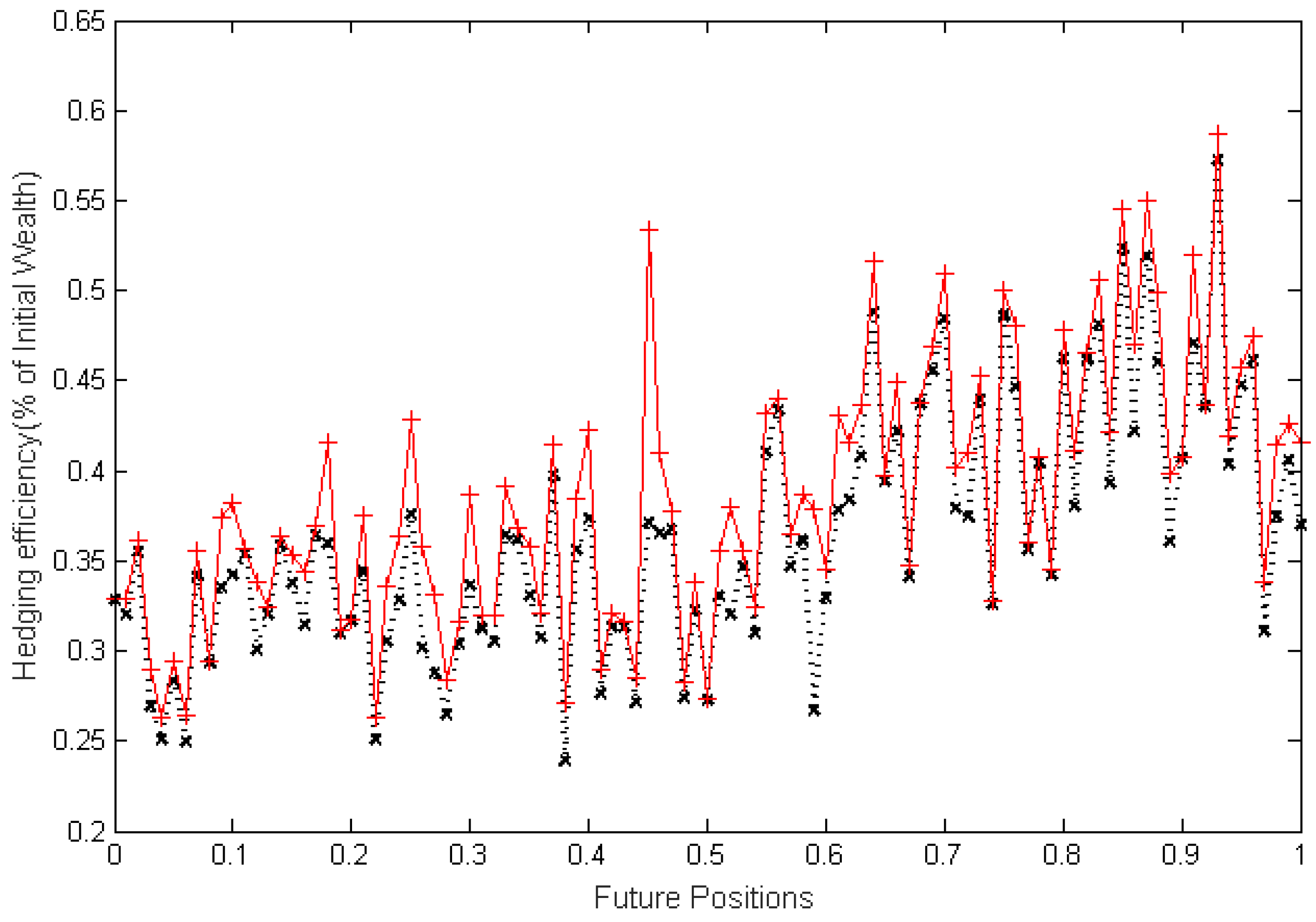
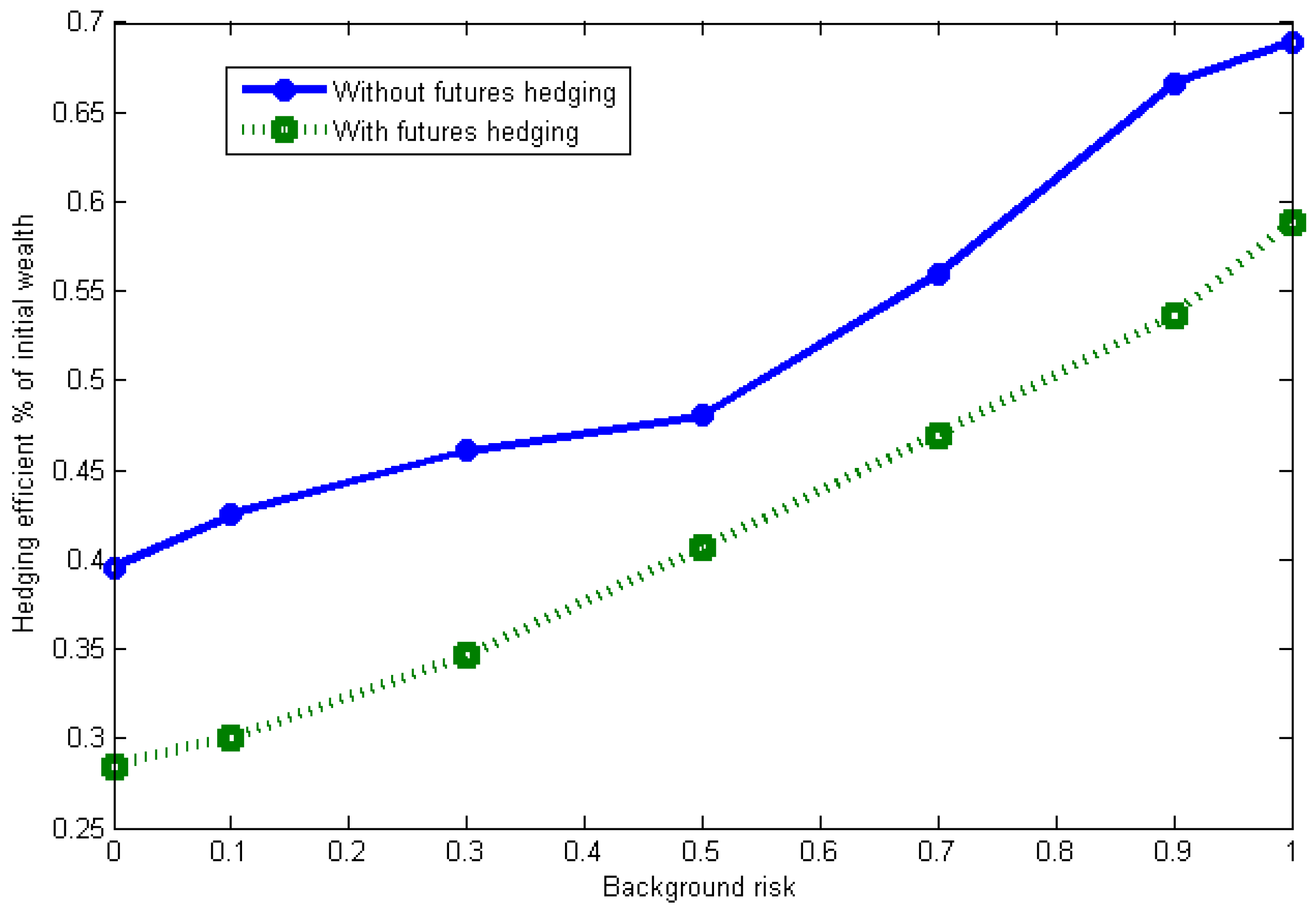
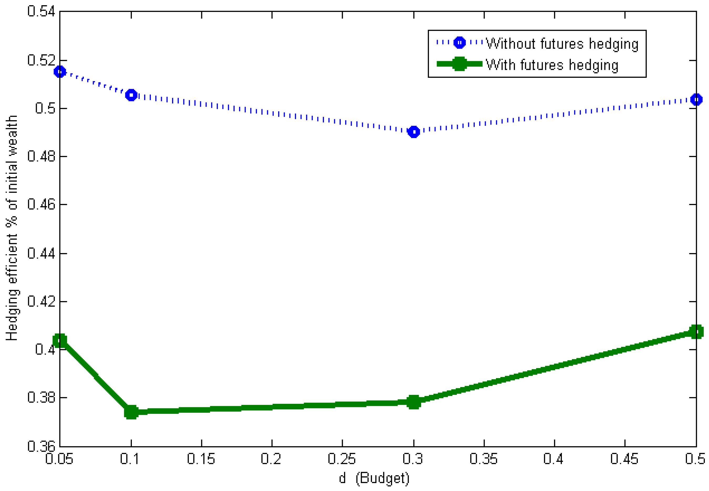
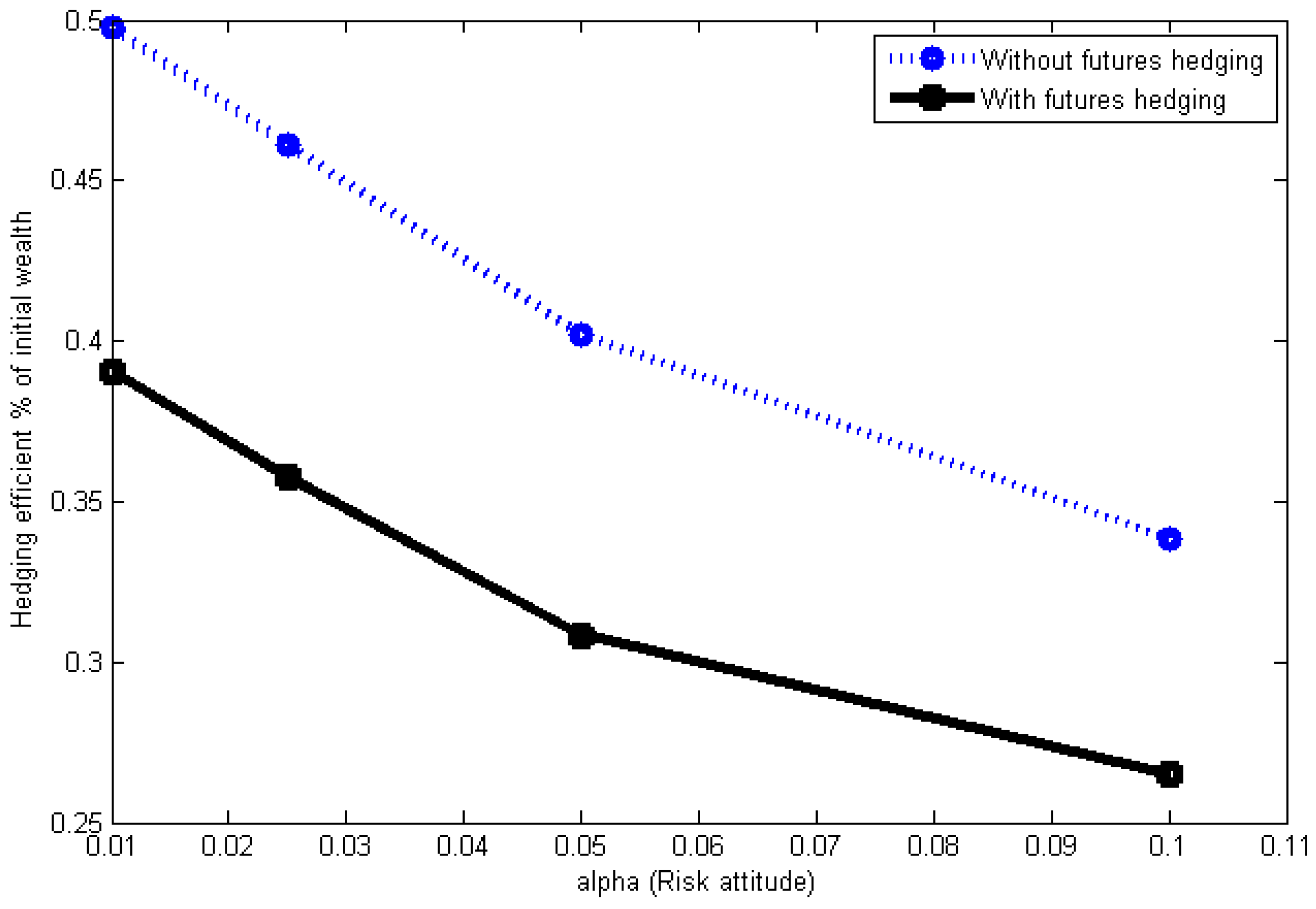
Section 4, we propose a simulation based on data of Shanghai 50 Exchange Traded Funds (SSE 50 ETF). in the Chinese market, and discuss the superiority by mixing futures hedging in minimizing ES. Based on the sensitivities, we provide some decision suggestions for the investors. Finally,
Section 5 concludes this paper.
3. Model
At the terminal date, an investor will sell quantity Q of a particular asset at random cash price . At the decision date (at time t), the investor can sell a discretionary fraction of Q amount of futures contracts at the future price , but she/he must repurchase them at the terminal date at the random future price . Simultaneously, the investor buys a discretionary fraction of amount of option contracts with options premium per contract denoted as Φ, and the terminal option value is denoted : if , and if .
Besides uncertainty prices of spots and futures, the firm also faces other sources of uncertainty aggregated into additive and/or multiplicative background risk, which is denoted as
, with a mean set equal to zero over support
, where
. Referring to Wong [
4], the terminal wealth is formulated as follows:
where
,
is a constant such that
. If
or 1, the background risk becomes purely additive or purely multiplicative, respectively. Some models in existing research are the special cases of this paper. For instance, when we set
and
, Equation (
1) is similar to the model of Bajo et al. [
1]. When we let
and
, and
is the spot exchange rate, the proposed model becomes the model of Wong [
33]; and the model of Wong [
34] is the special case when we assume that
and
. When we restrict the budget
and particular background risk forms, there are amounts of special models (see e.g., Broll and Zilcha [
35] and Lence [
36]). Our results offer new insights in the context of multiple uncertainties. Note that in Equation (
1), the option are not necessarily written on the spot, and we choose options on futures due to the higher liquidity of options on futures.
3.1. Optimal Hedging Decisions under the General Utility
Suppose that
is the loss of the hedged portfolio, where
. The utility function based on the loss satisfies
and
. Assume that the investor spends
C on buying put options. Namely,
. Then, the option positions can be calculated as
. Here,
Q and
C are known as constants rather than decision variables. Suppose that there is one period with two time instants, 0 and 1. For the sake of simplicity, we do not take the production costs into consideration. Hence, we discuss revenue rather than profit. The objective of the investor is to minimize the expected utility at time 1 under some constraints. It can be expressed by Problem (P1):
In the following, we study the optimal hedging problem under the framework of . We first derive the necessary and sufficient conditions that guarantee the optimality of an under-hedge , a full-hedge and an over-hedge of the futures in the following Propositions.
Proposition 2. Assume that there is no arbitrage in the market, if the investor’s utility function based on the loss satisfies and , then the optimal position of futures is smaller than, equal to, or greater than one, if and only if,is positive, zero, or negative, respectively. Proof. The first-order conditions of Program
corresponding to H is given by
One the other hand, differentiating
with respect to
H, and evaluating the resulting derivative at
yields
Due to no arbitrage in the market, we have
. Then, Equation (
3) can be rewritten as follows:
It follows from Equations (2) and (4) and the second-order conditions for Program
that
is less than, equal to, or greater than 1 if, and only if, the right-hand side of Equation (
4) is negative, zero, or positive, respectively. The following proposition stipulates sufficient condition under which an over-hedge
is optimal. ☐
Proposition 3. Assume that there is no arbitrage and no basis risk in the market, if the investor’s utility function satisfies and , the investor optimally opts an over-hedge, that is , if the random price and the background risk are independent.
Proof. From the results of Proposition 2, we need to prove that the right-hand of Equation (
4) is positive under the given conditions. In fact,
where Equation (
5) follows from the properties of the covariance operator
. (For any two random variables,
and,
,
) Therefore, the sign of Equation (
5) is the same as
. In fact,
Then, the strict convex of the utility implies that Equation (
6) is indeed negative. Under the same assumptions, Wong [
4] gave the result of full-hedge. However, in this paper, the result is over-hedge for futures positions. One of the main reasons is that only futures hedging in the model of Wong [
4], and both futures and options are involved in our model. It follows from Proposition 3 that the optimal position of futures is increased because of options hedging.
A natural question is why we add futures into the model of Bajo et al. [
1]. The next proposition shows the efficiency of our extension in minimizing the utility based on the loss or in maximizing the utility based on the profit. ☐
Proposition 4. Assume that there is no arbitrage and no basis risk. Let and be the optimal utility corresponding to with and without futures hedging and L is the loss. If the investor’s utility function satisfies with and , then implies that . In this case, it is always optimal for the risk averse investor to over-hedge futures relative to the case of only with options hedging.
Proof. We rewrite the random loss
L as
where
and 0 denote the cases with and without futures, respectively. The Problem
is given by
where
is defined in Equation (
7). The objective function of Problem
is convex due to
and
. Therefore, the first-order condition for Problem
is both necessary and sufficient for a unique maximum. Fix
, where
is the optimal strike price when there is no futures hedging. Treating
a as a continuous variable on the real line, it follows from risk aversion that
is convex in
a. Differentiating
with respect to
a and evaluating at
yields
where
Returning to Equation (
7) and using the assumption of no arbitrage in the market, we see that
Since
is decreasing with respect to
,
If the investor chooses over-hedge, i.e.,
, then Equation (
10) is negative. Furthermore, Equation (
9) is positive. Thus, the convexity of
in
a implies that
. Since
is the optimal solution to Problem
for
, it must be true that
. It then follows that inequality
holds. ☐
In the following, we examine the problem of minimizing ES with lognormal prices.
3.2. Optimal Hedging Decisions under Minimizing Risk of ES
In general, it is not impossible to characterize the explicit solutions without specific assumptions on the utility function and the distributions of the random variables. Thus, similar to Bajo et al. [
1], we propose the following assumptions: (i) the utility function of the investor is the risk measure of ES, which is also labelled as
in this paper, since we have proved that they are equivalent to each other; (ii) the random variables are used with lognormal dynamics for both the spot and the crossed futures, i.e.,
and
are standard correlated normal random variables with correlation matrix equal to
is the spot price at current time t, μ and are expected return, σ and are volatility. Zero mean normal distribution for the background risk over support . The correlation coefficient between background risk and spot price is set as .
We investigate how to solve the problem of minimizing
. Let
C be the budget of the investor to buy put options. Formally, the optimization problem can be written as Problem
:
where
is expressed as Equation (
1). In this paper, we study how the investor can optimally choose an option contract to minimize the risk exposure under the constraint of budget using Monte Carlo Simulation to solve the Problem
.
5. Conclusions
In this paper, we investigate the optimal hedging problem with futures and options. In the proposed model, futures hedging, options hedging and background risk are considered. We extend the previous research by allowing the simultaneous hedging choice of futures and options. We show a potentially important role of futures when there are price risks be it additive or multiplicative background risk. Upon comparison, we find that our model performs better than the previous approach in increasing the hedging efficiency. Some interesting results and practical implications are obtained in this paper. Theoretically, we present the necessary and sufficient conditions that guarantee the optimality of an under-hedge, a full-hedge, and an over-hedge. It stipulates sufficient conditions under which an over-hedge is optimal under the assumptions of no basis risk and a general utility. We also give the conditions when it is beneficial to hedge both with futures and options compared to hedging only with options. Practically, hedging with futures combined with options receives remarkable lower ES. The results demonstrate that our intention of adding futures in the model of Bajo et al. [
1] is advisable. We find that the optimal contract is affected by the amount of cash spent on the hedging, which is contrary to the existing literature of Ahn et al. [
36], but it is consistent with Bajo et al. [
1]. Another important factor that we have considered is the background risk. The results show that we especially can not ignore the multiplying background risk.
In futures hedging, we do not consider the opportunity cost and market-to-market risk in futures markets. However, in practice, reserve margin is not always able to maintain the required level, and the need is higher than that stipulated in the exchange level as margin of reserves. Excessive reserve margin restricts the investor from using money, and increases the opportunity cost of investors, while low standby margin may bring losses to investors. Therefore, as future work, we are planning to consider opportunity cost and market-to-market risk.


