
Analysis of Inflection and Singular Points on a Parametric Curve with a Shape Factor


Abstract
:1. Introduction
2. The Cubic Parametric Curve with a Shape Factor
3. Geometric Features of the Space Cubic Curve
4. Geometric Features of the Planar Cubic Curve
4.1. Edge Vectors and Are Non-Parallel
4.1.1. About the Cusp
4.1.2. About the Inflection Point
4.1.3. About the Double Point
4.1.4. About the Convexity
4.2. Edge Vectors and Are Parallel
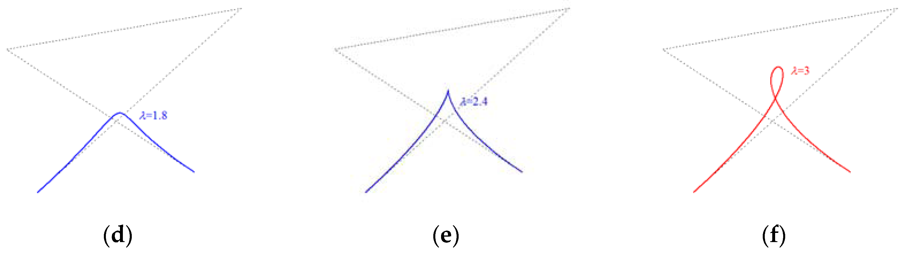
4.2.1. About the Cusp
4.2.2. About the Inflection Point
4.2.3. About the Double Point
- (1)
- The cubic parametric curve of has no cusp or double point.
- (2)
- If, and only if, when (i.e., the direction of is the same as that of ), the cubic parametric curve has one and only one, inflection point, otherwise the four control points are collinear.
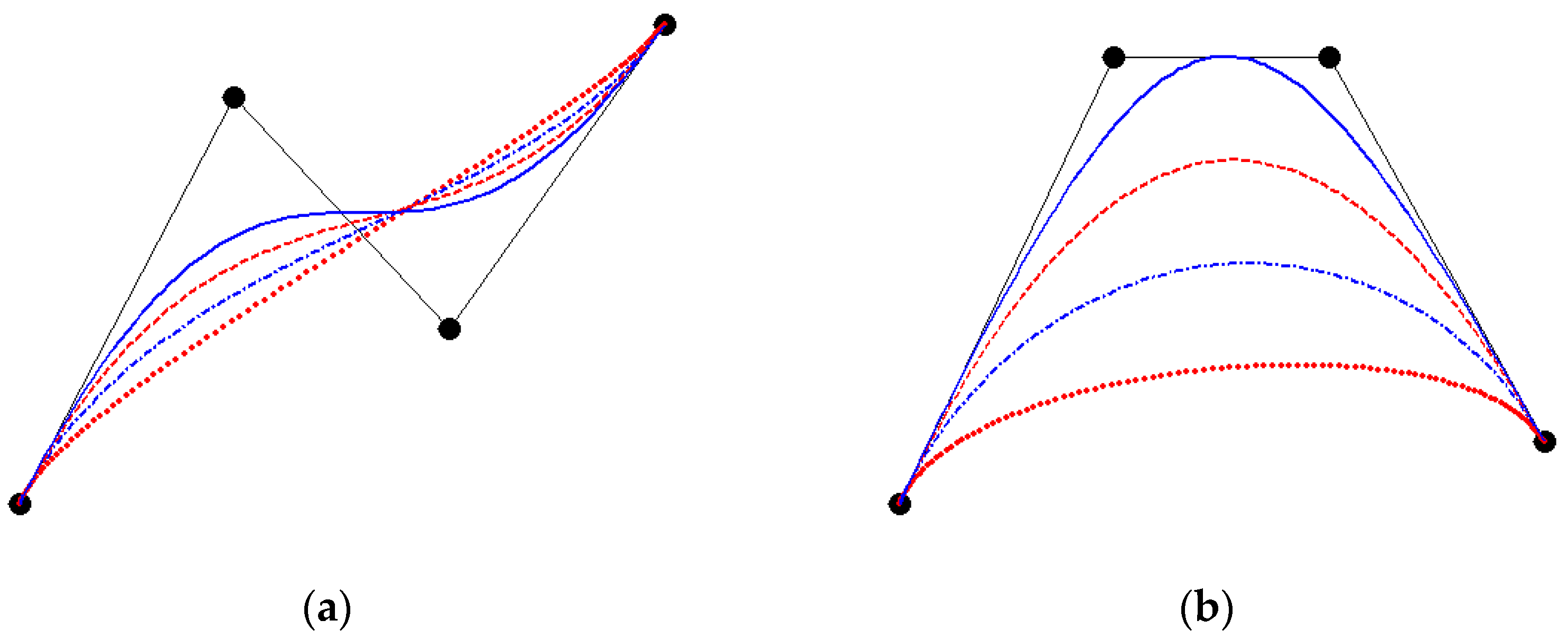
5. The Influence of the Shape Factor on the Cubic Parametric Curve
- (1)
- Shape distribution of the cubic parametric curve is symmetric about the straight line .
- (2)
- When , the cubic parametric curve reduces to a straight line, and the effect of shape factor disappears. When , degenerates into the Ball curve. If , degenerates into the cubic Bézier curve.
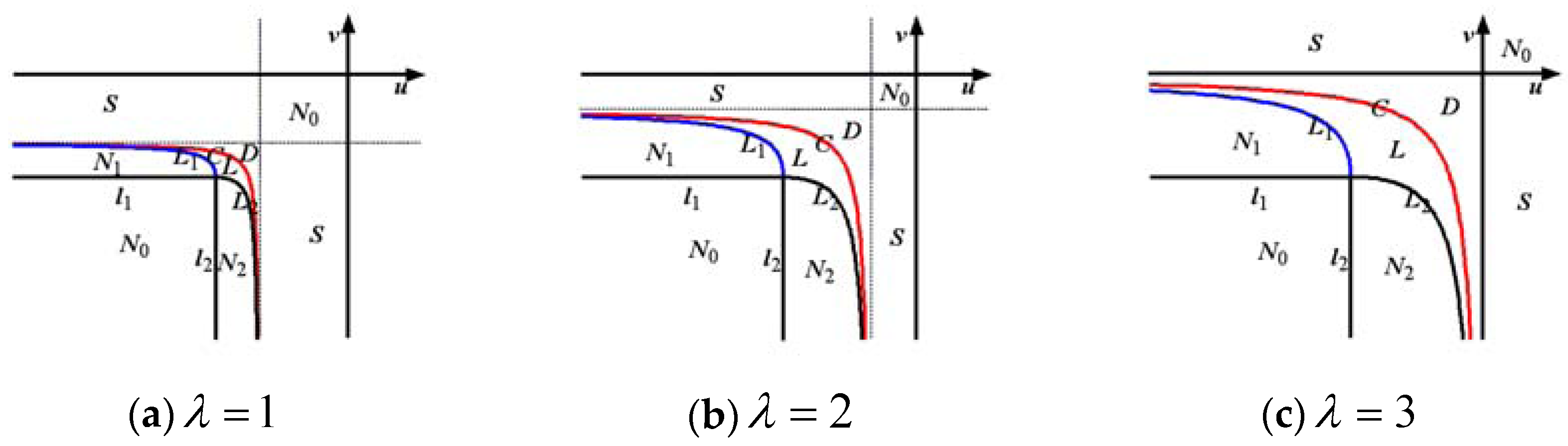
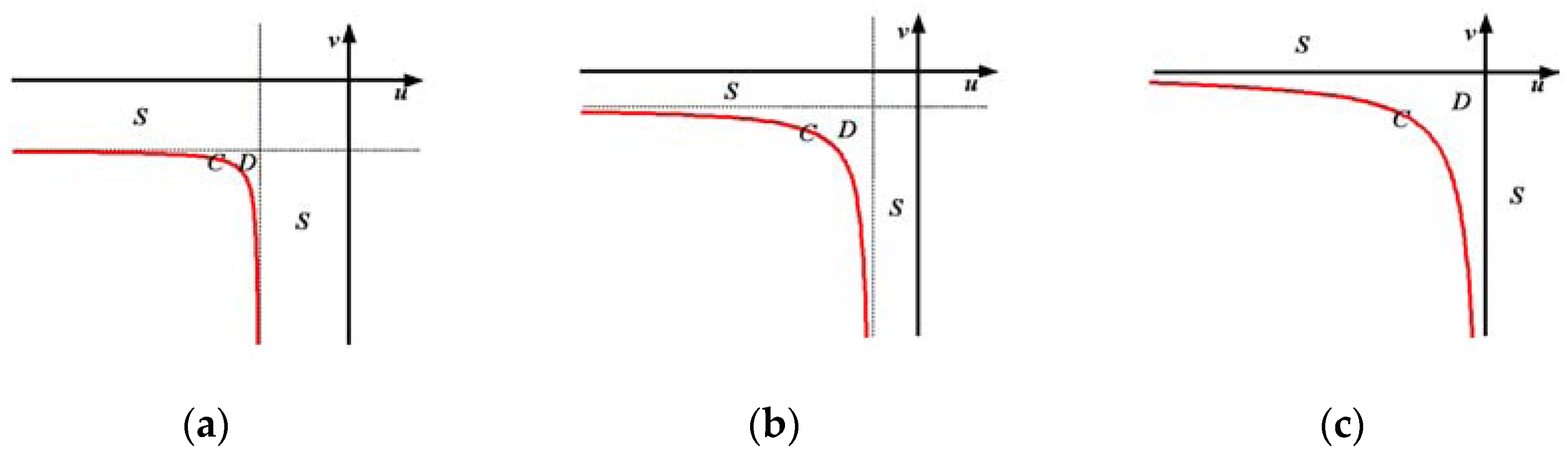
- (3)
- As the shape factor increases, the curve is drawn towards the origin , the curve is pulled toward the u-axis, and is pulled toward the v-axis. Thus, the region and decrease, and the regions , , and increase gradually.
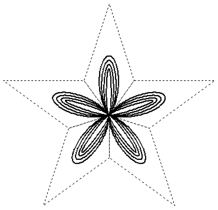
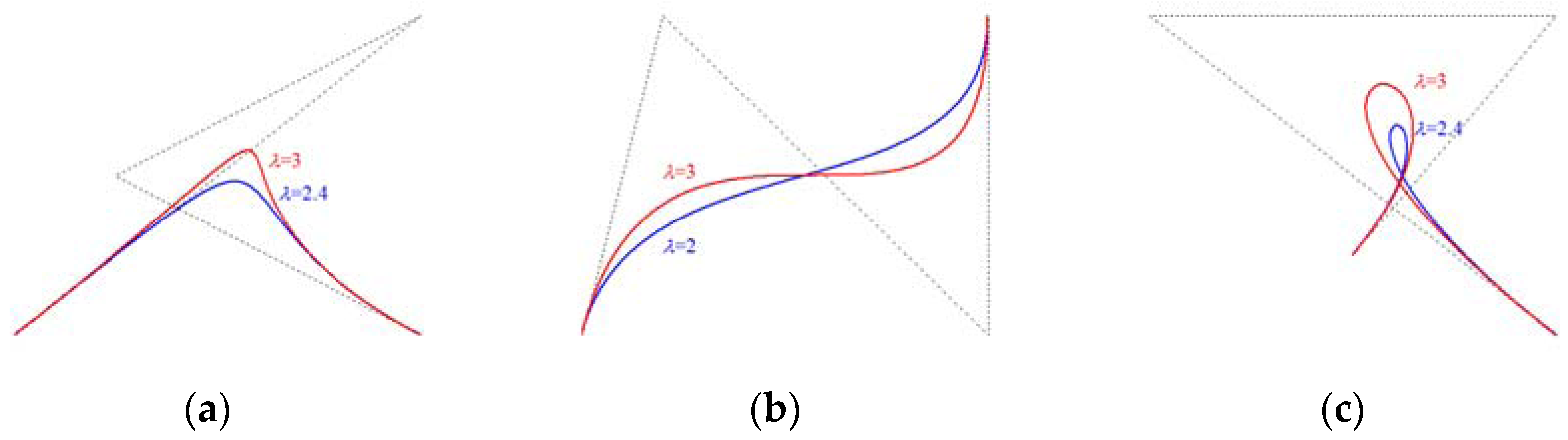
- (4)
- Whenthen the first edge and the last edge of the control polygon intersects (except that the first point and the last point coincide), there are likely singularity points, single inflection points, or double inflection points on the curve . Additionally, the curve may also be globally convex, but cannot be locally convex. Adjusting the shape factor can make the curve become a global convex curve.
6. Conclusions
Acknowledgments
Author Contributions
Conflicts of Interest
References
- Goldman, R.; Simeonov, P. Two essential properties of (q, h)-Bernstein-Bézier curves. Appl. Numer. Math. 2015, 96, 82–93. [Google Scholar] [CrossRef]
- Bézier, P. UNISURE, from styling to tool-shop. Comput. Ind. 1983, 4, 115–126. [Google Scholar] [CrossRef]
- Ball, A.A. CONSURF Part 1: Introduction of the Conic Lofting Title. Comput.-Aided Des. 1974, 6, 243–349. [Google Scholar] [CrossRef]
- Ball, A.A. CONSURF Part 2: Description of the Algorithms. Comput.-Aided Des. 1975, 7, 237–242. [Google Scholar] [CrossRef]
- Ball, A.A. CONSURF Part 3: How the program is used. Comput.-Aided Des. 1977, 9, 9–12. [Google Scholar] [CrossRef]
- Said, H.B. A generalized Ball curve and its recursive algorithm. ACM Trans. Graph. 1989, 4, 360–378. [Google Scholar] [CrossRef]
- Savetseranee, D.; Dejdumrong, N. Monomial forms of two generalized ball curves and their proofs. In Proceedings of the 2013 10th International Joint Conference on Computer Science and Software Engineering (JCSSE), KhonKaen, Thailand, 29–31 May 2013; pp. 235–239.
- Goodman, T.N.T.; Said, H.B. Properties of two types of generalized Ball curves and surfaces. Comput.-Aided Des. 1991, 23, 554–560. [Google Scholar] [CrossRef]
- Goodman, T.N.T.; Said, H.B. Shape-preserving properties of the generalized Ball basis. Comput.-Aided Des. 1991, 8, 115–121. [Google Scholar] [CrossRef]
- Kim, D.S. Hodograph approach to geometric characterization of parametric cubic curves. Comput.-Aided Des. 1993, 25, 644–654. [Google Scholar] [CrossRef]
- Li, Y.M.; Cripps, R.J. Identification of inflection points and cusps on rational curves. Comput.-Aided Des. 1997, 14, 491–497. [Google Scholar] [CrossRef]
- Manocha, D.; Canny, J.F. Detecting cusps and inflection points in curves. Comput. Aided Geom. Des. 1992, 9, 1–24. [Google Scholar] [CrossRef]
- Yang, Q.; Wang, G. Inflection points and singularities on C-curves. Comput. Aided Geom. Des. 2004, 21, 207–213. [Google Scholar] [CrossRef]
- Juhász, I. On the singularity of a class of parametric curves. Comput. Aided Geom. Des. 2006, 23, 146–156. [Google Scholar] [CrossRef]
- Stone, M.C.; DeRose, T.D. A geometric characterization of parametric cubic curves. ACM Trans. Graph. 1989, 8, 147–163. [Google Scholar] [CrossRef]
- OruÇ, H.; Phillips, G.M. q-Bernstein polynomials and Bézier curves. J. Comput. Appl. Math. 2003, 151, 1–12. [Google Scholar] [CrossRef]
- Timmer, H.G. Alternative representation for parametric cubic curves and surfaces. Comput.-Aided Des. 1980, 12, 25–28. [Google Scholar] [CrossRef]
- Han, X.A.; Huang, X.L.; Ma, Y.C. Shape analysis of cubic trigonometric Bézier curves with a shape parameter. Appl. Math. Comput. 2010, 217, 2527–2533. [Google Scholar] [CrossRef]


| Shape Features of the Plane Cubic Parametric Curve | ||||
|---|---|---|---|---|
| Convexity | Cusp | Double Point | Inflection Point | |
| / | one | no | no | |
| / | no | one | no | |
| / | no | no | one | |
| / | no | no | two | |
| global convexity | no | no | no | |
| local convexity | no | no | no | |
© 2017 by the authors; licensee MDPI, Basel, Switzerland. This article is an open access article distributed under the terms and conditions of the Creative Commons Attribution (CC-BY) license (http://creativecommons.org/licenses/by/4.0/).
Share and Cite
Liu, Z.; Li, C.; Tan, J.; Chen, X. Analysis of Inflection and Singular Points on a Parametric Curve with a Shape Factor. Math. Comput. Appl. 2017, 22, 9. https://doi.org/10.3390/mca22010009
Liu Z, Li C, Tan J, Chen X. Analysis of Inflection and Singular Points on a Parametric Curve with a Shape Factor. Mathematical and Computational Applications. 2017; 22(1):9. https://doi.org/10.3390/mca22010009
Chicago/Turabian StyleLiu, Zhi, Chen Li, Jieqing Tan, and Xiaoyan Chen. 2017. "Analysis of Inflection and Singular Points on a Parametric Curve with a Shape Factor" Mathematical and Computational Applications 22, no. 1: 9. https://doi.org/10.3390/mca22010009
APA StyleLiu, Z., Li, C., Tan, J., & Chen, X. (2017). Analysis of Inflection and Singular Points on a Parametric Curve with a Shape Factor. Mathematical and Computational Applications, 22(1), 9. https://doi.org/10.3390/mca22010009