The Analysis of Nonlinear Vibrations of Top-Tensioned Cantilever Pipes Conveying Pressurized Steady Two-Phase Flow under Thermal Loading

Abstract

This paper studied the nonlinear vibrations of top-tensioned cantilevered pipes conveying pressurized steady two-phase flow under thermal loading. The coupled axial and transverse governing partial differential equations of motion of the system were derived based on Hamilton’s mechanics, with the centerline assumed to be extensible. Using the multiple-scale perturbation technique, natural frequencies, mode shapes, and first order approximate solutions of the steady-state response of the pipes were obtained. The multiple-scale assessment reveals that at some frequencies the system is uncoupled, while at some frequencies a 1:2 coupling exists between the axial and the transverse frequencies of the pipe. Nonlinear frequencies versus the amplitude displacement of the cantilever pipe, conveying two-phase flow at super-critical mixture velocity for the uncoupled scenario, exhibit a nonlinear hardening behavior; an increment in the void fractions of the two-phase flow results in a reduction in the pipe’s transverse vibration frequencies and the coupled amplitude of the system. However, increases in the temperature difference, pressure, and the presence of top tension were observed to increase the pipe’s transverse vibration frequencies without a significant change in the coupled amplitude of the system.

1. Introduction

Two-phase flow is a common flow phenomenon in various industrial pipes: in nuclear heat exchangers, pipes in process plants, thermal plants, subsea oil and gas explorations, and many more. However, in spite of the vast occurrences of two-phase flow in pipes, most of the existing publications on the flow-induced vibrations of pipes conveying fluids focus on the fluidelastic instability of pipes conveying single-phase flow. Miwa et al. [1] did an in-depth review of the extent of existing work on two-phase flow-induced vibrations, stating that there exist very few results on the instability behavior of pipes due to internal two-phase flow. In the review, it was explained that internal two-phase flow-induced vibration can be initiated by various hydrodynamic phenomena; depending on the geometrical configurations of the flow channels and operating conditions, gas–liquid two-phase flow may create vibrations with various modes of amplitude and frequency. Monette and Pettigrew [2] presented an excellent experimental work on the fluidelastic instability of flexible tubes subjected to two-phase flow which might be one of the premier papers on the dynamics of pipes conveying two-phase flow and also reveals the relationship between the void fraction and the linear dynamics of the pipe for a two-phase liquid–gas flow. The early studies on the nonlinear dynamics of cantilevered pipes conveying single-phase flow either studied only the transverse displacement of the pipe or considered the longitudinal displacement using inextensible centerline assumptions [3,4,5]. However, the pioneering work by Ghayesh et al. [6] studied the nonlinear dynamics of a cantilevered extensible pipe conveying fluid, with equations of motion of the coupled transverse and longitudinal displacements derived using the Lagrange equations for a system containing non-material volumes, and highlighted that, conversely to inextensible pipe, an extensible pipe elongates in the axial direction as the flow velocity increases.

Luczko et al. [7] highlighted that the dynamic behavior of continuous systems, such as beams, moving tapes, or pipes with flowing fluid is governed by non-linear partial differential equations with appropriate boundary and initial conditions. As highlighted by Païdoussis [8], the nonlinear problems of pipes conveying fluids cannot be resolved analytically, but recourse needs to be taken to adopt specialized analytical methods like perturbation techniques, numerical time difference methods, or a combined analytical–numerical method. The direct Lagrangian discretization method (Galerkin method) to convert the partial differential equations (PDEs) to ordinary differential equations (ODEs) and then resolve the resulting ODEs using numerical techniques has been adopted by some publications, namely, Modarres and Païdoussis [9], Wang et al. [10], Sinir [11], Ritto et al. [12], Chen et al. [13], Tian-Zhi et al. [14]. The usage of analytical methods like perturbation techniques is highly common with researchers working on nonlinear problems, such as Nayfeh [15], Nayfeh [16], Kesimli et al. [17], and Oz and Boyaci [18], where the solutions were sought using an asymptotic expansion or by perturbing the original set of equations in terms of a small parameter which is either present in the equation or introduced artificially. Some researchers working on the fluidelastic instability of pipes conveying fluids have adopted this technique to resolve the nonlinear dynamics of the pipes, including the works of Enz [19] on a simple supported straight pipe using perturbation analysis with a multiple time-scaled method and comparison with measurements made by Coriolis flowmeters; the study by Xiao-Dong et al. [20] on the dynamic stability simply-supported viscoelastic pipe in transverse vibration for conveying pulsating fluid; the study on the transverse vibrations of tension pipes conveying fluid with time-dependent velocity using the multiple-scale perturbation technique by Oz and Pakdemirli [21]; and the study on the analysis of nonlinear vibrations of a pipe conveying an ideal fluid by Sinir and Demir [22].

Most of these existing publications on the nonlinear dynamics of a cantilevered pipe conveying fluid were focused on single-phase flow, resolving the governing equations using various methods as highlighted in the review of literature. However, profound among authors who adopted the perturbation approach is the study of the uncoupled problem, solving only the transverse vibrations independent of the axial vibration. To the best of our knowledge, a perturbation approach for the resolution of the coupled nonlinear dynamics of a top-tensioned cantilevered pipe conveying pressurized two-phase flow under thermal loading is still a reserved topic with a possibly intriguing outcome. In this paper, the governing equation of motion for the nonlinear coupled axial and transverse vibrations of a cantilever pipe conveying two-phase flow is derived and resolved by imposing the multiple-scale perturbation technique directly to the system equations (direct-perturbation method).

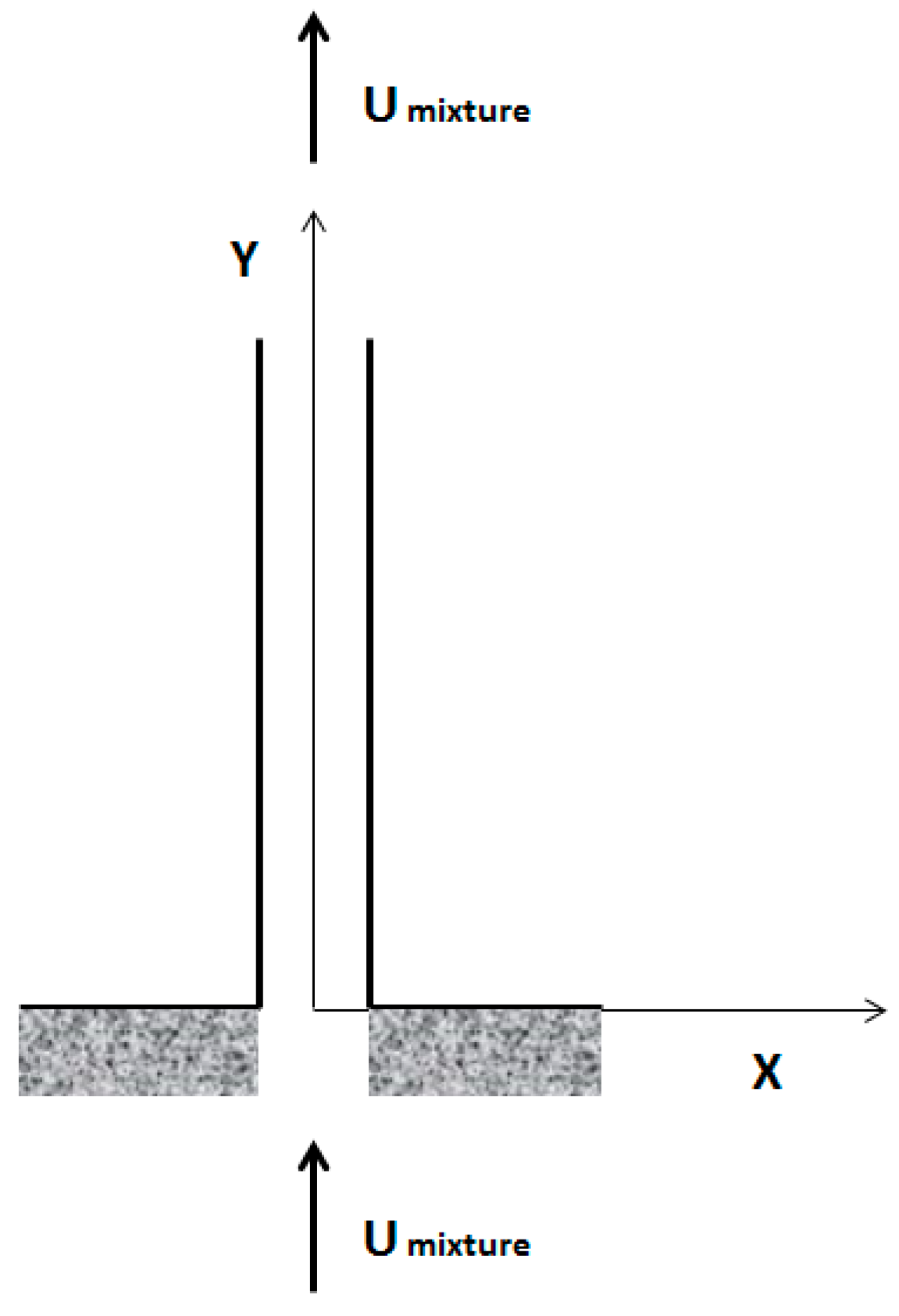
2. Problem Formulation and Modelling

Consider a system comprising a cantilever cylindrical pipe of length (L), having a cross-sectional area (A), mass per unit length (m_p) and flexural rigidity (EI), conveying multiphase flow, flowing parallel to the pipe’s centerline. The centerline axis of the pipe in its undeformed state is assumed to overlap with the Y-axis, and the cylinder is assumed to vibrate in the (Y, X) plane (see Figure 1). To derive the system’s governing equations of motion, the following basic assumptions were made for the cylinder and the fluid: (i) the mean flow velocity is constant; (ii) the cylinder is slender, so that the Euler–Bernoulli beam theory is applicable; (iii) although the deflections of the cylinder may be large, the strains are small; and (iv) the cylinder centerline is extensible.

The centerline of the cantilever pipe is assumed to be extensible to account for possible expansion due to the high temperature of the fluid content. The strain expressions and the geometric relation of the centerline of an extensible pipe are derived as expressed by Semler et al. [3].

2.1. Derivation of the Equation of Motion

The equations of motion are derived using the energy method. The energy method is based on Hamilton’s principle, which is defined as the variations of the time derivative of the Lagrangian. This can be mathematically expressed as

$$\delta {{\displaystyle \int }}_{t1}^{t2}ℒdt={{\displaystyle \int }}_{t1}^{t2}{\displaystyle \sum }_{j=1}^n{M}_j{U}_j\left({\dot{r}}_L+{\displaystyle \sum }_{j=1}^n{U}_j{\tau }_L\right)\delta r_{L}dt$$

(1)

where $n$ is the number of phases in the fluid, which will be 2 for a two-phase flow;

• $M_j$ is the mass of the phases in the fluid;
• $U_j$ is the flow velocity of the phases in the fluid; and
• $ℒ$ is the Lagrangian operator expressed in Equation (2):

  $$ℒ={\mathcal{T}}_f+{\mathcal{T}}_p-{\mathcal{V}}_f-{\mathcal{V}}_p$$

  (2)

where ${\mathcal{T}}_p\mathrm{and}{\mathcal{V}}_p$ are the kinetic and potential energies of the pipe, respectively, and ${\mathcal{T}}_f\mathrm{and}{\mathcal{V}}_f$ are the kinetic and potential energies associated with the conveyed fluid, respectively.

The following expressions hold: ${\dot{r}}_L={\dot{u}}_{L}i+{\dot{v}}_{L}k$ and ${\tau }_L={u^{\prime }}_{L}i+{v^{\prime }}_{L}k$.

2.1.1. Kinetic Energy

The total kinetic energy of the system is the summation of the kinetic energy of the pipe and the kinetic energies of the phases/components of the flowing fluid. The velocity vector of the pipe’s centerline is expressed as

$${\overrightarrow{V}}_p=\frac{\partial u}{\partial t}\widehat{i}+\frac{\partial v}{\partial t}\widehat{j}.$$

(3)

Therefore, the kinetic energy of the pipe is expressed as

$${\mathcal{T}}_p=\frac{1}{2}{m}_p{{\displaystyle \int }}_0^L\left[{\left(\frac{\partial u}{\partial t}\right)}^2+{\left(\frac{\partial v}{\partial t}\right)}^2\right]dx.$$

(4)

As illustrated by Semler, the axial elongation of the pipe is complemented by a lateral contraction, due to the Poisson effect. This will impact the flow velocity of the fluid phases/components such that

$${\displaystyle \sum }_{j=1}^n{U}_j=\left[\left(1+ϵ\right)/\left(1+aϵ\right)\right]{\displaystyle \sum }_{j=1}^n{U_0}_j$$

(5)

where ${U_0}_j\mathrm{and}{U}_j$ are the flow velocities before and after elongation, the subscript (j) is used to identify the various phases/components of the conveyed fluid, $\left(ϵ\right)$ is the axial strain, and $\left(a\right)$ relates to the Poisson ratio ($v$) as $a=1-2v$; for an extreme case, $v=0.5$ and $a$becomes zero, as in Ghayesh et al. [6].

The flow velocity relative to the centerline axis of the pipe is expressed as

$${\overrightarrow{V}}_f=\left\{\frac{\partial u}{\partial t}+{\displaystyle \sum }_{j=1}^n{U}_j\left(1-aϵ\right)\left(1+\frac{\partial u}{\partial x}\right)\right\}\widehat{i}+\left\{\frac{\partial v}{\partial t}+{\displaystyle \sum }_{j=1}^n{U}_j\left(1-aϵ\right)\left(\frac{\partial v}{\partial x}\right)\right\}\widehat{j}.$$

(6)

Therefore, the Kinetic energy of the conveyed fluid is expressed as

$${\mathcal{T}}_f=\frac{1}{2}{\displaystyle \sum }_{j=1}^n{M}_j{{\displaystyle \int }}_0^L\left\{{\left(\frac{\partial u}{\partial t}\right)}^2+{\left(\frac{\partial v}{\partial t}\right)}^2+U_j{}^2\left[1+2\frac{\partial u}{\partial x}+{\left(\frac{\partial u}{\partial x}\right)}^2-2a\left(\frac{\partial u}{\partial x}+\frac{1}{2}{\left(\frac{\partial v}{\partial x}\right)}^2\right)+{\left(\frac{\partial v}{\partial x}\right)}^2\right]+2U_j\left[\frac{\partial u}{\partial t}\left(1+\frac{\partial u}{\partial x}\right)+\frac{\partial v}{\partial t}\frac{\partial v}{\partial x}\right]\right\}dx.$$

(7)

2.1.2. Potential Energy

Semler highlighted that the potential energy is a result of the elastic deformation of the pipe and the effect of gravity, and the deformation from elastic behavior of the pipe can be linked to the strain energy. This is expressed as

$${\mathcal{V}}_p=\frac{1}{2}EA{{\displaystyle \int }}_0^L{ϵ}^{2}dx+\frac{1}{2}EI{{\displaystyle \int }}_0^L{\left(1+ϵ\right)}^2{k}^{2}dx.$$

(8)

This is clearly the combination of the axial strain effect and the bending strain effect where (E) denotes the Young’s modulus, (I) denotes the pipe moment of inertia, (A) denotes the cross-sectional area, $\left(ϵ\right)$ is the axial strain, and (k) is the curvature term as expressed by Semler.

The thermal effect can be introduced by considering the linear strain tensor as a sum of the strain contributions from the mechanical stress and the thermal effect. Semler further decomposed the axial strain into a steady strain component due to externally applied tension $\left(T_0\right)$, a pressure force component $\left(P=pA\right)$, and an oscillatory strain component due to the oscillations of the pipe. These can be expressed as

$${ϵ}_{ij}={ϵ}_{ij}{}^{\sigma }+{ϵ}_{ij}{}^{\Delta }+\frac{T_0-P}{EA}$$

(9)

while the stress-contributing strain component is as expressed by Semler as

$${ϵ}_{ij}{}^{\sigma }=\frac{\partial u}{\partial x}-\frac{1}{2}\left(\frac{\partial u}{\partial x}\right){\left(\frac{\partial v}{\partial x}\right)}^2+\frac{1}{2}{\left(\frac{\partial v}{\partial x}\right)}^2-\frac{1}{8}{\left(\frac{\partial v}{\partial x}\right)}^4.$$

(10)

We note that the gradient of the transverse displacement of the pipe is far greater than the gradient of the longitudinal displacement$\left(\frac{\partial v}{\partial x}>\frac{\partial u}{\partial x}\right)$. Also, the thermal contributing strain component can be expressed in terms of the thermal expansivity ($\alpha$) and the difference in temperatures ($\Delta T$) as

$${ϵ}_{ij}{}^{\Delta }=\left(-\alpha \Delta T\right).$$

(11)

Substituting Equations (10) and (11) into Equation (9), and then substituting Equation (9) into Equation (8), the resulting expression is

$${\mathcal{V}}_p=\frac{1}{2}EA{{\displaystyle \int }}_0^L{\left[\left(u^{\prime }-\frac{1}{2}{u}^{\prime }{v}^{\prime }{}^2+\frac{1}{2}{v^{\prime }}^2-\frac{1}{8}{v^{\prime }}^4\right)+\frac{T_0-P}{EA}+\left(-\alpha \Delta T\right)\right]}^{2}dx+\frac{1}{2}EI{{\displaystyle \int }}_0^L\left[{v^{″}}^2-2{v^{″}}^2{u}^{\prime }-2{v^{″}}^2{u^{″}}^2-2v^{\prime }{v}^{″}{u}^{″}\right]dx.$$

(12)

With the reference plane in the same direction as the gravitational acceleration, the effect of gravity can be expressed as

$${\mathcal{V}}_g=g\left({\displaystyle \sum }_{j=1}^n{M}_j+m\right){{\displaystyle \int }}_0^L\left(x+u\right)dx.$$

(13)

The variations of the time derivative of the algebraic sum of the kinetic energy and the potential energy of the systems gives the expression on the left-hand side term of Hamilton’s equation.

2.1.3. Non-Conservative Work Done

As detailed by Semler for a single-phase flow, the right-hand side term of Hamilton’s equation can be expressed for a multiphase flow as

$$EI{v^{‴}}_L={\displaystyle \sum }_{j=1}^n{M}_j{U}^2{}_j{{\displaystyle \int }}_{t1}^{t2}{v^{\prime }}_L\delta vdt.$$

(14)

Physically, this implies a non-classical boundary condition at the free end for a discharging cantilever pipe. Therefore, a force is imposed at the free end if the velocity of the exiting fluid is not tangential to the pipe. However, this study assumes that the exiting flow remains tangential to the pipe at the free end, and therefore the classical boundary condition holds at the free end.

2.2. Equation of Motion for Multiphase Flow

The equation of motion for an extensible cantilever pipe conveying pressurized unsteady multiphase flow under thermal loading can be expressed as

$$\begin{array}{ll}\left(m+{\displaystyle {\displaystyle \sum }_{j=1}^n}{M}_j\right)\ddot{u}& +{\displaystyle {\displaystyle \sum }_{j=1}^n}{M}_j\dot{U_j}+{\displaystyle {\displaystyle \sum }_{j=1}^n}2M_j{U}_j{\dot{u}}^{\prime }+{\displaystyle {\displaystyle \sum }_{j=1}^n}{M}_j{U}_j{}^2{u}^{″}+{\displaystyle {\displaystyle \sum }_{j=1}^n}{M}_j\dot{U_j}{u}^{\prime }-EA{u}^{″}\\ & -EI\left(v^{\prime \prime \prime \prime }{v}^{\prime }+v^{″}{v}^{‴}\right)+\left(T_0-P-EA\left(\alpha \Delta T\right)-EA\right)v^{\prime }{v}^{″}\\ & -{\left(T_0-P-EA\left(\alpha \Delta T\right)\right)}^{\prime }+\left(m+{\displaystyle {\displaystyle \sum }_{j=1}^n}{M}_j\right)g=0,\end{array}$$

(15)

$$\begin{array}{ll}\left(m+{\displaystyle {\displaystyle \sum }_{j=1}^n}{M}_j\right)\ddot{v}+& {\displaystyle {\displaystyle \sum }_{j=1}^n}2M_j{U}_j{\dot{v}}^{\prime }+{\displaystyle {\displaystyle \sum }_{j=1}^n}{M}_j{U}_j{}^2{v}^{″}-{\displaystyle {\displaystyle \sum }_{j=1}^n}a{M}_j{U}_j{}^2{v}^{″}+{\displaystyle {\displaystyle \sum }_{j=1}^n}{M}_j\dot{U_j}{v}^{\prime }+EI{v}^{\prime \prime \prime \prime }\\ & -\left(T_0-P-EA\left(\alpha \Delta T\right)\right)v^{″}\\ & -EI\left(3u^{‴}{v}^{″}+4v^{‴}{u}^{″}+2u^{\prime }{v}^{\prime \prime \prime \prime }+2{v^{\prime }}^2{v}^{\prime \prime \prime \prime }+8v^{\prime }{v}^{″}{v}^{‴}+2{v^{″}}^3\right)\\ & +\left(T_0-P-EA\left(\alpha \Delta T\right)-EA\right)\left(u^{\prime }{v}^{″}+v^{\prime }{u}^{″}+\frac{3}{2}{v^{\prime }}^2{v}^{″}\right)=0.\end{array}$$

(16)

The associated boundary conditions are

$$v\left(0\right)=v^{\prime }\left(0\right)\mathrm{and}{v}^{″}\left(L\right)=v^{‴}\left(L\right)=0,$$

(17)

$$u\left(0\right)=u^{\prime }\left(L\right)=0.$$

(18)

Dimensionless Equation of Motion for Two-Phase Flow

The equation of motion may be rendered dimensionless to make the analysis of the system more robust and not constrained to one specific system by introducing the following non-dimensional quantities:

$$\overline{u}=\frac{u}{L},\overline{v}=\frac{v}{L},\overline{t}={\left[\frac{EI}{{{\displaystyle \sum }}^{\text{}}{M}_j+m}\right]}^{\raisebox{1ex}{$1$}\!\left/ \!\raisebox{-1ex}{$2$}\right.}\frac{t}{L^2},{\overline{U}}_j={\left[\frac{M_j}{EI}\right]}^{\raisebox{1ex}{$1$}\!\left/ \!\raisebox{-1ex}{$2$}\right.}UL,\gamma =\frac{{{\displaystyle \sum }}^{\text{}}{M}_j+m}{EI}{L}^{3}g,$$

$${\beta }_j=\frac{M_j}{{{\displaystyle \sum }}^{\text{}}{M}_j+m},{\Psi }_j=\frac{M_j}{{{\displaystyle \sum }}^{\text{}}{M}_j},\mathrm{Damping}\mathrm{term}:\mu =\frac{C{L}^2}{\sqrt{{{\displaystyle \sum }}^{\text{}}\left(M_j+m\right)}EI}$$

$$\mathrm{Tension}:{\Pi }_0=\frac{T_o{L}^2}{EI},\mathrm{Flexibility}:{\Pi }_1=\frac{EA{L}^2}{EI},\mathrm{Pressure}:{\Pi }_2=\frac{P{L}^2}{EI}.$$

The dimensionless governing equation can be reduced to that of a two-phase as follows:

$$\begin{array}{ll}\ddot{\overline{u}}+\dot{\overline{U_1}}\sqrt{{\Psi }_1}\sqrt{{\beta }_1}+& \dot{\overline{U_2}}\sqrt{{\Psi }_2}\sqrt{{\beta }_2}+2{\overline{U}}_1\sqrt{{\Psi }_1}\sqrt{{\beta }_1}{\dot{\overline{u}}}^{\prime }+2{\overline{U}}_2\sqrt{{\Psi }_2}\sqrt{{\beta }_2}{\dot{\overline{u}}}^{\prime }+{\Psi }_1{\overline{U_1}}^2{\overline{u}}^{″}\\ & +{\Psi }_2{\overline{U_2}}^2{\overline{u}}^{″}+\dot{\overline{U_1}}\sqrt{{\Psi }_1}\sqrt{{\beta }_1}{\overline{u}}^{\prime }+\dot{\overline{U_2}}\sqrt{{\Psi }_2}\sqrt{{\beta }_2}{\overline{u}}^{\prime }-{\Pi }_1{\overline{u}}^{″}\\ & -\left({\overline{v}}^{″″}{\overline{v}}^{\prime }+{\overline{v}}^{″}{\overline{v}}^{‴}\right)+\left({\Pi }_0-{\Pi }_2-{\Pi }_1\left(\alpha \Delta T\right)-{\Pi }_1\right){\overline{v}}^{\prime }{\overline{v}}^{″}\\ & -{\left({\Pi }_0-{\Pi }_2-{\Pi }_1\left(\alpha \Delta T\right)\right)}^{\prime }+\gamma =0,\end{array}$$

(19)

$$\begin{array}{ll}\ddot{\overline{v}}+2{\overline{U}}_1\sqrt{{\Psi }_1}\sqrt{{\beta }_1}{\dot{\overline{v}}}^{\prime }& +2{\overline{U}}_2\sqrt{{\Psi }_2}\sqrt{{\beta }_2}{\dot{\overline{v}}}^{\prime }+{\Psi }_1{\overline{U_1}}^2{\overline{v}}^{″}+{\Psi }_2{\overline{U_2}}^2{\overline{v}}^{″}-a{\Psi }_1{\overline{U_1}}^2{\overline{v}}^{″}-a{\Psi }_2{\overline{U_2}}^2{\overline{v}}^{″}\\ & +\dot{\overline{U_1}}\sqrt{{\Psi }_1}\sqrt{{\beta }_1}{\overline{v}}^{\prime }+\dot{\overline{U_2}}\sqrt{{\Psi }_2}\sqrt{{\beta }_2}{\overline{v}}^{\prime }-\left({\Pi }_0-{\Pi }_2-{\Pi }_1\left(\alpha \Delta T\right)\right)v^{″}+{\overline{v}}^{″″}\\ & -\left(3{\overline{u}}^{‴}{\overline{v}}^{″}+4{\overline{v}}^{‴}{\overline{u}}^{″}+2{\overline{u}}^{\prime }{\overline{v}}^{″″}+2{\overline{v}}^{\prime }{}^2{\overline{v}}^{″″}+8{\overline{v}}^{\prime }{\overline{v}}^{″}{\overline{v}}^{‴}+2{\overline{v}}^{″}{}^3\right)\\ & +\left({\Pi }_0-{\Pi }_2-{\Pi }_1\left(\alpha \Delta T\right)-{\Pi }_1\right)\left({\overline{u}}^{\prime }{\overline{v}}^{″}+{\overline{v}}^{\prime }{\overline{u}}^{″}+\frac{3}{2}{\overline{v}}^{\prime }{}^2{\overline{v}}^{″}\right)=0.\end{array}$$

(20)

For a steady flow, velocities are not changing with time, therefore

$$\dot{\overline{U_1}}=\dot{\overline{U_2}}=0.$$

(21)

We define the following notation:

$$C11=\sqrt{{\Psi }_1}\sqrt{{\beta }_1},C12=\sqrt{{\Psi }_2}\sqrt{{\beta }_2},C21=2\sqrt{{\Psi }_1}\sqrt{{\beta }_1},$$

$$C22=2\sqrt{{\Psi }_2}\sqrt{{\beta }_2},C31={\Psi }_1,C32={\Psi }_2,C5={\Pi }_1,$$

$$C6=({\Pi }_0-{\Pi }_2-{\Pi }_1\left(\alpha \Delta T\right)-{\Pi }_1),C7={\Pi }_0-{\Pi }_2-{\Pi }_1\left(\alpha \Delta T\right).$$

The governing equation for a cantilevered pipe conveying steady two-phase flow can be expressed as

$$\ddot{\overline{u}}+{\overline{U}}_{1}C21{\dot{\overline{u}}}^{\prime }+{\overline{U}}_{2}C22{\dot{\overline{u}}}^{\prime }+C31{\overline{U_1}}^2{\overline{u}}^{″}+C32{\overline{U_2}}^2{\overline{u}}^{″}-C5{\overline{u}}^{″}-\left({\overline{v}}^{″″}{\overline{v}}^{\prime }+{\overline{v}}^{″}{\overline{v}}^{″\prime }\right)+C6{\overline{v}}^{\prime }{\overline{v}}^{″}-C{7}^{\prime }+\gamma )=0,$$

(22)

$$\begin{array}{l}\ddot{\overline{v}}+{\overline{U}}_{1}C21{\dot{\overline{v}}}^{\prime }+{\overline{U}}_{2}C22{\dot{\overline{v}}}^{\prime }+C31{\overline{U_1}}^2{\overline{v}}^{″}+C32{\overline{U_2}}^2{\overline{v}}^{″}-aC31{\overline{U_1}}^2{\overline{v}}^{″}-aC32{\overline{U_2}}^2{\overline{v}}^{″}-C7v^{″}+{\overline{v}}^{″″}\\ -\left(3{\overline{u}}^{‴}{\overline{v}}^{″}+4{\overline{v}}^{‴}{\overline{u}}^{″}+2{\overline{u}}^{\prime }{\overline{v}}^{″″}+2{\overline{v}}^{\prime }{}^2{\overline{v}}^{″″}+8{\overline{v}}^{\prime }{\overline{v}}^{″}{\overline{v}}^{‴}+2{\overline{v}}^{″}{}^3\right)\\ +C6\left({\overline{u}}^{\prime }{\overline{v}}^{″}+{\overline{v}}^{\prime }{\overline{u}}^{″}+\frac{3}{2}{\overline{v}}^{\prime }{}^2{\overline{v}}^{″}\right)=0.\end{array}$$

(23)

The dimensionless boundary conditions are

$$\overline{v}\left(0\right)={\overline{v}}^{\prime }\left(0\right)\mathrm{and}{\overline{v}}^{″}\left(L\right)={\overline{v}}^{‴}\left(L\right)=0,$$

(24)

$$\overline{u}\left(0\right)={\overline{u}}^{\prime }\left(L\right)=0.$$

(25)

In these equations, $\overline{u}\mathrm{and}\overline{v}$ are, respectively, the dimensionless displacements in the longitudinal and transverse direction; $({\overline{U}}_j)$ is the flow velocities of the constituent phases/components used in the parametric studies of the dynamics of the system; $({\beta }_j)$ is the same mass ratio as in single-phase flows as derived by Semler and Paidoussis [8]; $({\Psi }_j)$ is another mass ratio which is unique to multiphase flow relating the fluid mass independent of the mass of the pipe; $\left(\gamma \right)$ is the gravity term; and $({\Pi }_0,{\Pi }_1,{\Pi }_2)$ represent the Tension term, Flexibility term, and the Pressurization term, respectively.

2.3. Empirical Gas–Liquid Two-Phase Flow Model

Adopting the Chisholm empirical relations as presented in [23], the void fraction is expressed as

$$vf={\left[1+\sqrt{1-x\left(1-\frac{{\rho }_l}{{\rho }_g}\right)}\left(\frac{1-x}{x}\right)\left(\frac{{\rho }_g}{{\rho }_l}\right)\right]}^{-1}=\frac{\mathrm{Volume}\mathrm{of}\mathrm{gas}}{\mathrm{Volume}\mathrm{of}\mathrm{gas}+\mathrm{Volume}\mathrm{of}\mathrm{Liquid}}.$$

(26)

The Slip Ratio is expressed as

$$S=\frac{V_g}{V_l}={\left[1-x\left(1-\frac{{\rho }_l}{{\rho }_g}\right)\right]}^{1/2}$$

(27)

where $x\mathrm{is}\mathrm{the}\mathrm{vapor}\mathrm{density};\mathrm{and}{\rho }_l,{\rho }_g\mathrm{are}\mathrm{the}\mathrm{densities}\mathrm{of}\mathrm{the}\mathrm{liquid}\mathrm{and}\mathrm{gas}\mathrm{phases},\mathrm{respectively}.$

Mixture Velocity is expressed as

$$V_T=U_{g}vf+U_l\left(1-vf\right)$$

(28)

where $U_g$ and $U_l$ are the superficial flow velocities.

Individual Velocities for the two phases can be expressed as

$$V_l=\frac{V_T}{S+1},V_g=\frac{S{V}_T}{S+1}.$$

(29)

For various void fractions (0.3, 0.4, and 0.5) and a series of mixture velocities, the corresponding slip ratio and individual velocities are estimated and used for numerical calculations.

3. Method of Solution

Exact solutions of nonlinear equations are almost always not available; an approximate solution will be sought by utilizing the multiple time-scale perturbation technique. This approach is applied directly to the partial differential Equations (22) and (23), given that the common method of discretizing the equations first and then applying the perturbation method yields less accurate results for finite mode truncations and higher order perturbation schemes [15,16,17,18].

Adopting perturbation techniques, it is necessary to decide the terms to be considered small or weak. This study considers the contributions of the nonlinear terms, gradient term and gravity term to be small compared to the linear terms.

$$\ddot{\overline{u}}+{\overline{U}}_{1}C21{\dot{\overline{u}}}^{\prime }+{\overline{U}}_{2}C22{\dot{\overline{u}}}^{\prime }+C31{\overline{U_1}}^2{\overline{u}}^{″}+C32{\overline{U_2}}^2{\overline{u}}^{″}-C5{\overline{u}}^{″}+\epsilon \left(-\left({\overline{v}}^{″″}{\overline{v}}^{\prime }+{\overline{v}}^{″}{\overline{v}}^{‴}\right)+C6{\overline{v}}^{\prime }{\overline{v}}^{″}-C{7}^{\prime }+{\gamma }_j\right)=0,$$

(30)

$$\begin{array}{l}\ddot{\overline{v}}+{\overline{U}}_{1}C21{\dot{\overline{v}}}^{\prime }+{\overline{U}}_{2}C22{\dot{\overline{v}}}^{\prime }+C31{\overline{U_1}}^2{\overline{v}}^{″}+C32{\overline{U_2}}^2{\overline{v}}^{″}-aC31{\overline{U_1}}^2{\overline{v}}^{″}-aC32{\overline{U_2}}^2{\overline{v}}^{″}-C7v^{″}+{\overline{v}}^{″″}\\ +\epsilon \left(-\left(3{\overline{u}}^{‴}{\overline{v}}^{″}+4{\overline{v}}^{‴}{\overline{u}}^{″}+2{\overline{u}}^{\prime }{\overline{v}}^{″″}+2{\overline{v}}^{\prime }{}^2{\overline{v}}^{″″}+8{\overline{v}}^{\prime }{\overline{v}}^{″}{\overline{v}}^{‴}+2{\overline{v}}^{″}{}^3\right)+C6\left({\overline{u}}^{\prime }{\overline{v}}^{″}+{\overline{v}}^{\prime }{\overline{u}}^{″}+\frac{3}{2}{\overline{v}}^{\prime }{}^2{\overline{v}}^{″}\right)\right)=0.\end{array}$$

(31)

We seek an approximate solution for $\overline{u}\mathrm{and}\overline{v}$ in the form

$$\overline{u}={\overline{u}}_0\left(T_0,T_1\right)+\epsilon {\overline{u}}_1\left(T_0,T_1\right)+{\epsilon }^2{\overline{u}}_2\left(T_0,T_1\right)+O\left(\epsilon \right),$$

(32)

$$\overline{v}={\overline{v}}_0\left(T_0,T_1\right)+\epsilon {\overline{v}}_1\left(T_0,T_1\right)+{\epsilon }^2{\overline{v}}_2\left(T_0,T_1\right)+O\left(\epsilon \right).$$

(33)

where $\epsilon$ is a small dimensionless measure of the amplitude of $\overline{u}$ and $\overline{v}$, used as a book-keeping parameter. Two time scales are needed: $T_0=t\mathrm{and}{T}_1=\epsilon t$. Then, the time derivatives are

$$\frac{d}{dt}=D_0+\mathsf{\epsilon }{D}_1+{\mathsf{\epsilon }}^2{D}_2+O\left(\epsilon \right),$$

(34)

$$\frac{d^2}{d{t}^2}=D_0{}^2+2\mathsf{\epsilon }{D}_0{D}_1+{\mathsf{\epsilon }}^2(D_1{}^2+2D_0{D}_2)+O\left(\epsilon \right)$$

(35)

where $D_n=\frac{\partial }{\partial T_n}$.

Substituting Equations (32)–(35) into Equations (30) and (31) and equating the coefficients of $\left(\epsilon \right)$ to zero and one, respectively, we get the following:

U-Equation:

$$O\left({\mathsf{\epsilon }}^0\right).D_0{}^2{\overline{u}}_0+C21D_0{\overline{u}}_0{}^{\prime }{\overline{U}}_1+C22D_0{\overline{u}}_0{}^{″}{\overline{U}}_2+C31{\overline{u}}_0{}^{″}{\overline{U}}_1{}^2+C32{\overline{u}}_0{}^{\prime }\prime {\overline{U}}_2{}^2-C5{\overline{u}}_0{}^{″}=0,$$

(36)

$$\begin{array}{ll}O\left({\mathsf{\epsilon }}^1\right).D_0{}^2{\overline{u}}_1+& C21D_0{\overline{u}}_1{}^{\prime }{\overline{U}}_1+C22D_0{\overline{u}}_1{}^{\prime }{\overline{U}}_2+2D_1{D}_0{\overline{u}}_0+C31{\overline{u}}_1{}^{″}{\overline{U}}_1{}^2+C32{\overline{u}}_1{}^{″}{\overline{U}}_2{}^2\\ & +C21D_0{\overline{u}}_0{}^{\prime }{\overline{U}}_1+C22D_0{\overline{u}}_0{}^{\prime }{\overline{U}}_2-C5{\overline{u}}_1{}^{″}-{\overline{v}}_0{}^{″″}{\overline{v}}_0{}^{\prime }-C{7}^{\prime }+\gamma \\ & -{\overline{v}}_0{}^{″}{\overline{v}}_0{}^{‴}+C6{\overline{v}}_0{}^{\prime }{\overline{v}}_0{}^{″}=0.\end{array}$$

(37)

V-Equation:

$$\begin{array}{ll}O\left({\mathsf{\epsilon }}^0\right).D_0{}^2{\overline{v}}_0-& C7{\overline{v}}_0{}^{″}+{\overline{v}}_0{}^{″″}+C21D_0{\overline{v}}_0{}^{\prime }{\overline{U}}_1+C22D_0{\overline{v}}_0{}^{\prime }{\overline{U}}_2+C31{\overline{v}}_0{}^{″}{\overline{U}}_1{}^2\\ & +C32{\overline{v}}_0{}^{″}{\overline{U}}_2{}^2-aC31{\overline{v}}_0{}^{″}{\overline{U}}_1{}^2-aC32{\overline{v}}_0{}^{″}{\overline{U}}_2{}^2=0,\end{array}$$

(38)

$$\begin{array}{ll}O\left({\mathsf{\epsilon }}^1\right).D_0{}^2{\overline{v}}_1-& C7{\overline{v}}_1{}^{″}+{\overline{v}}_1{}^{″″}-2{\overline{u}}_0{}^{\prime }{\overline{v}}_0{}^{″″}-4{\overline{u}}_0{}^{″}{\overline{v}}_0{}^{‴}-3{\overline{v}}_0{}^{″}{\overline{v}}_0{}^{‴}-2{\overline{v}}_0{{}^3}^{″}\\ & +2D_0{D}_1{\overline{v}}_0+C31{\overline{v}}_1{}^{″}{\overline{U}}_1{}^2+C32{\overline{v}}_1{}^{″}{\overline{U}}_2{}^2-8{\overline{v}}_0{}^{\prime }{\overline{v}}_0{}^{″}{\overline{v}}_0{}^{‴}+C6{\overline{u}}_0{}^{\prime }{\overline{v}}_0{}^{″}\\ & +C6{\overline{u}}_0{}^{″}{\overline{v}}_0{}^{\prime }+\frac{3}{2}C6{\overline{v}}_0{{}^2}^{\prime }{\overline{v}}_0{}^{″}+C21D_0{\overline{v}}_0{}^{\prime }{\overline{U}}_1+C22D_0{\overline{v}}_0{}^{\prime }{\overline{U}}_2\\ & +C21D_1{\overline{v}}_0{}^{\prime }{\overline{U}}_1+C22D_1{\overline{v}}_0{}^{\prime }{\overline{U}}_2-aC31{\overline{v}}_1{}^{″}{\overline{U}}_1{}^2-aC32{\overline{v}}_1{}^{″}{\overline{U}}_2{}^2=0.\end{array}$$

(39)

The order zero problems for both the axial and transverse vibration of the cantilever pipe have the form of an undamped and unforced flow-induced vibration problem; this will be used to estimate the linear natural frequencies and mode shapes, while the order one problem will be solved to obtain the amplitude of the nonlinear response of the pipe.

3.1. Linear Analysis

The leading order equations present a set of linear equations which relates the flow velocity-generated forces (Coriolis and Centrifugal forces) to the stiffness of the pipe without neglecting the mass ratios. This set of linear equations exhibits the form of an eigenvalue problem, which upon resolution will produce the natural frequency and mode shapes, and also predict the stability of the system.

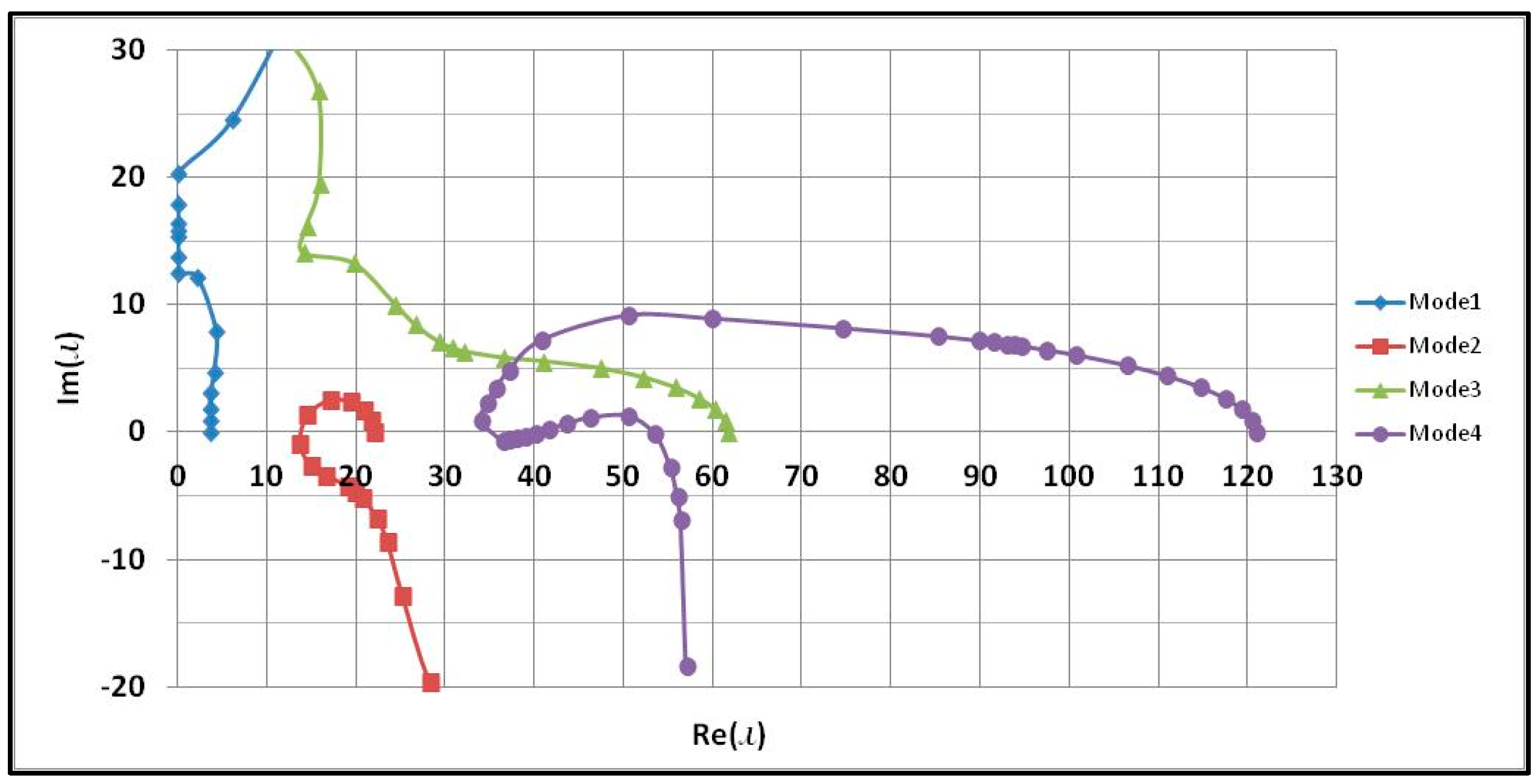
3.1.1. Natural Frequencies and Modal Functions

Estimation of the natural frequencies and modal function is an order zero problem that can be determined by resolving Equations (36) and (38).

The homogeneous solution of the leading order Equations (36) and (38) can be expressed as

$$\overline{u}{\left(x,T_0,T_1\right)}_0=\varphi {\left(x\right)}_{n}exp\left(i{\omega }_n{T}_0\right)+CC,$$

(40)

$$\overline{v}{\left(x,T_0,T_1\right)}_0=\eta {\left(x\right)}_{n}exp\left(i{\lambda }_n{T}_0\right)+CC$$

(41)

where $\left(CC\right)$ is the complex conjugate, $\varphi {\left(x\right)}_n\mathrm{and}\eta {\left(x\right)}_n$are the complex modal functions for the axial and transverse vibrations for each mode (n), and ${\omega }_n\mathrm{and}{\lambda }_n$ are the eigenvalues for the axial and transverse vibrations for each mode (n).

The eigenvalues are complex values with a complex conjugate pair of solutions which can be expressed as

$${\omega }_n=Re({\omega }_n)+iIm({\omega }_n)\mathrm{and}\overline{{\omega }_n}=Re({\omega }_n)-iIm({\omega }_n),$$

$${\lambda }_n=Re({\omega }_n)+iIm({\lambda }_n)\mathrm{and}\overline{{\lambda }_n}=Re({\lambda }_n)-iIm({\lambda }_n).$$

The real parts of the eigenvalues are associated with the natural frequency of oscillation, and the imaginary parts with the damping.

Substituting Equations (40) and (41) into Equations (36) and (38), respectively, results in

$$\left(C31{\overline{U}}_1{}^2+C32{\overline{U}}_2{}^2-C5\right)\varphi {\left(x\right)}_n{}^{″}+\left(C21{\overline{U}}_1+C22{\overline{U}}_2\right)i{\omega }_n\varphi {\left(x\right)}_n{}^{\prime }-\varphi {\left(x\right)}_n{\omega }_n{}^2=0,$$

(42)

$$\eta {\left(x\right)}_n{}^{″″}+\left(C31{\overline{U}}_1{}^2+C32{\overline{U}}_2{}^2-C7-aC31{\overline{U}}_1{}^2-aC32{\overline{U}}_2{}^2\right)\eta {\left(x\right)}_n{}^{″}+\left(C21{\overline{U}}_1+C22{\overline{U}}_2\right)i{\lambda }_n\eta {\left(x\right)}_n{}^{\prime }-\eta {\left(x\right)}_n{\lambda }_n{}^2=0.$$

(43)

The general solution to the ordinary differential Equations (42) and (43) is expressed as

$$\varphi {\left(x\right)}_n=G{1}_{n}exp\left(i{k}_{1}x\right)+G{2}_{n}exp\left(i{k}_{2}x\right),$$

(44)

$$\eta {\left(x\right)}_n=H1(exp\left(i{z}_{1}x\right)+H2exp\left(i{z}_{2}x\right)+H3exp\left(i{z}_{3}x\right)+H4exp\left(i{z}_{4}x\right)).$$

(45)

3.1.2. Solution to Axial Vibration Problem

Substituting Equation (44) into Equation (42) gives a quadratic relation of the form

$$\left(C5-C31{\overline{U}}_1{}^2-C32{\overline{U}}_2{}^2\right)k_j{}^2-\left(C21{\overline{U}}_1+C22{\overline{U}}_2\right)i{\omega }_n{k}_j-{\omega }_n{}^2=0.$$

(46)

We solve the quadratic Equation (46) for the wave numbers $(k_j)$ as a function of the eigenvalue $\left({\omega }_n\right)$:

$$k_1=a\left({\omega }_n\right),$$

(47)

$$k_2=b\left({\omega }_n\right)$$

(48)

In order to obtain the eigenvalue, Equation (51) is substituted into the boundary conditions in Equation (25):

$$G1+G2=0$$

(49)

and

$$G1k1iexp\left(iL{k}_1\right)+G2k2iexp\left(iL{k}_2\right)=0.$$

(50)

In matrix form:

$$\underset{D}{\underbrace{\left(\begin{array}{c}11\\ i{k}_{1}exp\left(iL{k}_1\right)i{k}_{2}exp\left(iL{k}_2\right)\end{array}\right)}}\left(\begin{array}{c}G1\\ G2\end{array}\right)=0.$$

(51)

For a non-trivial solution, the determinant of (D) must varnish:

$$-i{k}_{1}exp\left(iL{k}_1\right)+i{k}_{2}exp\left(iL{k}_2\right)=0.$$

(52)

We substitute Equations (47) and (48) into Equation (52) and solve for the eigenvalue:

$${\omega }_n=\frac{2\pi n-i·ln\left(\frac{b}{a}\right)}{\left(a-b\right)L},n=1,2,3,\dots$$

(53)

where

$$a=\frac{\frac{C21{\overline{U}}_1}{2}+\frac{C22{\overline{U}}_2}{2}+\frac{\sqrt{C{21}^2{\overline{U}}_1{}^2+2C21C22{\overline{U}}_1{\overline{U}}_2+C{22}^2{\overline{U}}_2{}^2-4C31{\overline{U}}_1{}^2-4C32{\overline{U}}_2{}^2+4C5}}{2}}{C5-C31{\overline{U}}_1{}^2-C32{\overline{U}}_2{}^2},$$

$$b=\frac{\frac{C21{\overline{U}}_1}{2}+\frac{C22{\overline{U}}_2}{2}-\frac{\sqrt{C{21}^2{\overline{U}}_1{}^2+2C21C22{\overline{U}}_1{\overline{U}}_2+C{22}^2{\overline{U}}_2{}^2-4C31{\overline{U}}_1{}^2-4C32{\overline{U}}_2{}^2+4C5}}{2}}{C5-C31{\overline{U}}_1{}^2-C32{\overline{U}}_2{}^2}.$$

Equation (53) is the pipe’s axial vibration eigenvalue. Solving Equations (49) and (50) gives the constants G1 and G2. Therefore, the modal function for the axial vibration of the pipe is expressed as

$$\varphi {\left(x\right)}_n=G{1}_{n}exp\left(i{k}_{1}x\right)+G{2}_{n}exp\left(i{k}_{2}x\right).$$

(54)

Substituting Equation (44) into Equation (40) yields

$$\overline{u}{\left(x,T_0\right)}_0={\displaystyle \sum }_{j=1}^2{G}_{jn}exp\left(i{k}_{jn}x\right)exp\left(i{\omega }_n{T}_0\right)={\displaystyle \sum }_{j=1}^2{G}_{jn}exp\left(-Im\left(k_{jn}x\right)-Im\left({\omega }_n{T}_0\right)\right)exp\left(i\left(Re\left(k_{jn}x\right)+Re\left({\omega }_n{T}_0\right)\right)\right).$$

(55)

It can be observed from Equation (55) that the real part is the natural frequency and the imaginary part is the amplitude. However, as the mixture velocity is varied, a critical value of the mixture velocity is attained when the imaginary parts of any of the eigenvalues $\left({\omega }_n\right)$ take on a negative value which will cause the axial displacement $\left(\overline{u}\right)$ to grow exponentially in time and linearly signifies the onset of the system’s oscillatory instability.

3.1.3. Solution to Transverse Vibration Problem

Substituting Equation (45) into Equation (43) gives a quartic relation:

$$z^4{}_{jn}+\left(C7-C31{\overline{U}}_1{}^2-C32{\overline{U}}_2{}^2+aC31{\overline{U}}_1{}^2+aC32{\overline{U}}_2{}^2\right)z^2{}_{jn}-\left(C21{\overline{U}}_1+C22{\overline{U}}_2\right)z_{jn}{\lambda }_n-{\lambda }^2{}_n=0$$

(56)

for j = 1, 2, 3, 4 and n = 1, 2, 3, 4, 5, …

In order to obtain the eigenvalue, Equation (45) is substituted into the boundary conditions in Equation (24).

This gives four algebraic equations which can be expressed in matrix form as

$$\underset{G}{\underbrace{\lfloor \begin{array}{cccc}1& 1& 1& 1\\ z_{1n}& z_{2n}& z_{3n}& z_{4n}\\ {\left(z_{1n}\right)}^2·\exp \left(i·z_{1n}\right)& {\left(z_{2n}\right)}^2·\exp \left(i·z_{2n}\right)& {\left(z_{3n}\right)}^2·\exp \left(i·z_{3n}\right)& {\left(z_{4n}\right)}^2·\exp \left(i·z_{4n}\right)\\ {\left(z_{1n}\right)}^3·\exp \left(i·z_{1n}\right)& {\left(z_{2n}\right)}^3·\exp \left(i·z_{2n}\right)& {\left(z_{3n}\right)}^3·\exp \left(i·z_{3n}\right)& {\left(z_{4n}\right)}^3·\exp \left(i·z_{4n}\right)\end{array}\rfloor }}·\left[\begin{array}{c}1\\ H{2}_n\\ H{3}_n\\ H{4}_n\end{array}\right]·H{1}_n=\left(\begin{array}{l}0\\ 0\\ 0\\ 0\end{array}\right).$$

(57)

For a non-trivial solution, the determinant of (G) must varnish, that is

$$DET\left(G\right)=0.$$

(58)

In order to find modal solutions of$\left({\lambda }_n\right)$, Equations (57) and (58) must be solved simultaneously; this can be solved numerically using a nonlinear numerical routine.

The mode function of the transverse vibration corresponding to the nth eigenvalue is expressed as

$$\mathsf{ƞ}{\left(x\right)}_n=H{1}_n·\left[e^{x·z_{1n}·i}-\left(A+B+C+D\right)-E\right],$$

(59)

$$A=\frac{e^{x·z_{4n}·i}·[e^{z_{1n}·i}·{\left(z_{1n}\right)}^3·z_{2n}-e^{z_{1n}·i}·{\left(z_{1n}\right)}^3·z_{3n}-e^{z_{1n}·i}·z_{4n}·{\left(z_{1n}\right)}^2·z_{2n}}{\left(z_{2n}-z_{4n}\right)·\left(z_{3n}-z_{4n}\right)·\left[e^{z_{2n}·i}·{\left(z_{2n}\right)}^2-e^{z_{3n}·i}·{\left(z_{3n}\right)}^2\right]},$$

$$B=\frac{e^{x·z_{4n}·i}·[e^{z_{1n}·i}·z_{4n}·{\left(z_{1n}\right)}^2·z_{3n}-e^{z_{2n}·i}·z_{1n}·{\left(z_{2n}\right)}^3+e^{z_{2n}·i}·z_{4n}·z_{1n}·{\left(z_{2n}\right)}^2}{\left(z_{2n}-z_{4n}\right)·\left(z_{3n}-z_{4n}\right)·\left[e^{z_{2n}·i}·{\left(z_{2n}\right)}^2-e^{z_{3n}·i}·{\left(z_{3n}\right)}^2\right]},$$

$$C=\frac{e^{x·z_{4n}·i}·[e^{z_3·i}·z_{1n}·{\left(z_{3n}\right)}^3-e^{z_3·i}·z_{4n}·z_{1n}·{\left(z_{3n}\right)}^2+e^{z_{2n}·i}·{\left(z_{2n}\right)}^3·z_{3n}}{\left(z_{2n}-z_{4n}\right)·\left(z_{3n}-z_{4n}\right)·\left[e^{z_{2n}·i}·{\left(z_{2n}\right)}^2-e^{z_{3n}·i}·{\left(z_{3n}\right)}^2\right]},$$

$$D=\frac{e^{x·z_{4n}·i}·[-e^{z_{2n}·i}·z_{4n}·{\left(z_{2n}\right)}^2·z_{3n}-e^{z_3·i}·z_{2n}·{\left(z_{3n}\right)}^3+e^{z_3·i}·z_{4n}·z_{2n·}{\left(z_{3n}\right)}^2}{\left(z_{2n}-z_{4n}\right)·\left(z_{3n}-z_{4n}\right)·\left[e^{z_{2n}·i}·{\left(z_{2n}\right)}^2-e^{z_{3n}·i}·{\left(z_{3n}\right)}^2\right]},$$

$$\begin{array}{l}E=\frac{e^{x·z_{2n}·i}·\left(z_{1n}-z_{4n}\right)·\left[e^{z_1·i}·{\left(z_{1n}\right)}^2-e^{z_3·i}·{\left(z_{3n}\right)}^2\right]}{\left(z_{2n}-z_{4n}\right)·\left[e^{z_2·i}·{\left(z_{2n}\right)}^2-e^{z_3·i}·{\left(z_{3n}\right)}^2\right]}\\ +\frac{e^{x·z_3·i}·\left(z_{1n}-z_{4n}\right)·\left[e^{z_{1n}·i}·{\left(z_{1n}\right)}^2-e^{z_{2}i}·{\left(z_{2n}\right)}^2\right]}{\left(z_{3n}-z_{4n}\right)·\left[e^{z_2·i}·{\left(z_{2n}\right)}^2-e^{z_3·i}·{\left(z_{3n}\right)}^2\right]}·\end{array}$$

Substituting Equation (45) into Equation (41) yields

$$\overline{v}{\left(x,T_0\right)}_0={\displaystyle \sum }_{j=1}^4{H}_{jn}exp\left(i{z}_{jn}x\right)exp\left(i{\lambda }_n{T}_0\right)={\displaystyle \sum }_{j=1}^4{H}_{jn}exp\left(-Im\left(z_{jn}x\right)-Im\left({\lambda }_n{T}_0\right)\right)exp\left(i\left(Re\left(z_{jn}x\right)+Re\left({\lambda }_n{T}_0\right)\right)\right).$$

(60)

It can be observed from Equation (60) that the real part is the natural frequency and the imaginary part is the amplitude. However, as the mixture velocity is varied, a critical value of the mixture velocity is attained when the imaginary parts of any of the eigenvalues $\left({\lambda }_n\right)$ take on a negative value which will cause the transverse displacement $\left(\overline{v}\right)$ to grow exponentially in time and linearly signifies the onset of the system’s flutter instability.

3.2. Nonlinear Analysis

Linear analysis of the system is sufficient for the prediction of the critical velocity at which instability will occur, but cannot predict the post-buckling behavior. Linear theory has shown that buckling amplitudes will grow unboundedly with time after the critical velocity, however, as amplitudes grow, the effect of nonlinearities comes into play. This predictably limits the growth to some finite value [24,25,26].

3.2.1. Nonlinear Axial and Transverse Vibration Problem

We solve the nonlinear axial and transverse vibration problem by seeking an approximate solution for $\overline{u}\mathrm{and}\overline{v}$ of the form

$$\overline{u}={\overline{u}}_0\left(T_0,T_1\right)+\epsilon {\overline{u}}_1\left(T_0,T_1\right)+{\epsilon }^2{\overline{u}}_2\left(T_0,T_1\right)+O\left(\epsilon \right),$$

(61)

$$\overline{v}={\overline{v}}_0\left(T_0,T_1\right)+\epsilon {\overline{v}}_1\left(T_0,T_1\right)+{\epsilon }^2{\overline{v}}_2\left(T_0,T_1\right)+O\left(\epsilon \right).$$

(62)

The zero order solutions produce the undamped and uncoupled linear solution of the axial and transverse vibrations, respectively:

$$\overline{u}{\left(x,T_0,T_1\right)}_0=\varphi \left(x\right)X\left(T_1\right)exp\left(i\omega T_0\right)+CC,$$

(63)

$$\overline{v}{\left(x,T_0,T_1\right)}_0=\eta \left(x\right)Y\left(T_1\right)exp\left(i\lambda T_0\right)+CC$$

(64)

where X and Y are unknown complex-valued functions of the slow time scale T₁, $\left(CC\right)$ is the complex conjugate, $\varphi \left(x\right)\mathrm{and}\eta \left(x\right)$ are the modal functions for the axial and transverse vibrations, and $\omega =Re\left(\omega \right)\mathrm{and}\lambda =Re\left(\lambda \right)$. (the real parts of the complex frequencies) are the natural frequencies for the axial and transverse vibrations.

Substituting Equations (63) and (64) into Equations (37) and (39) gives

$$D_0{}^2{\overline{u}}_1-C5{\overline{u}}_1{}^{″}+C21D_0{\overline{u}}_1{}^{\prime }{\overline{U}}_1+C22D_0{\overline{u}}_1{}^{\prime }{\overline{U}}_2+C31{\overline{u}}_1{}^{″}{\overline{U}}_1{}^2+C32{\overline{u}}_1{}^{″}{\overline{U}}_2{}^2=-Q1·\left[\frac{\partial X\left(T1\right)}{\partial T1}\right]exp\left(i\omega T_0\right)+Q2·\left[Y{\left(T1\right)}^2\right]exp\left(2i\lambda T_0\right)+NST+CC=0,$$

(65)

$$\begin{array}{ll}{D}_0{}^2{\overline{v}}_1-C7{{\overline{v}}_1}^{″}+{\overline{v}}_1{}^{″″}& +C21D_0{\overline{v}}_1{}^{\prime }{\overline{U}}_1+C22D_0{\overline{v}}_1{}^{\prime }{\overline{U}}_2+C31{\overline{v}}_1{}^{″}{\overline{U}}_1{}^2+C32{\overline{v}}_1{}^{″}{\overline{U}}_2{}^2-aC31{\overline{v}}_1{}^{″}{\overline{U}}_1{}^2\\ & -aC32{\overline{v}}_1{}^{″}{\overline{U}}_2{}^2\\ & =\left(Q3·\left[\frac{\partial Y\left(T1\right)}{\partial T1}\right]+Q4·\left[Y{\left(T1\right)}^2\overline{Y\left(T1\right)}\right]\right)exp\left(i\lambda T_0\right)\\ & +Q5·\left[X\left(T1\right)\overline{Y\left(T1\right)}\right]exp\left(i\omega T_0\right)exp\left(-i\lambda T_0\right)+Q6·\left[Y{\left(T1\right)}^2\right]exp\left(2i\lambda T_0\right)+NST+CC\\ & =0,\end{array}$$

(66)

where

$$\begin{array}{l}Q1=C21\frac{\partial \varphi \left(x\right)}{\partial x}{\overline{U}}_1+C22\frac{\partial \varphi \left(x\right)}{\partial x}{\overline{U}}_2+2i\varphi \left(x\right)\omega ,\\ Q2=\frac{\partial \eta \left(x\right)}{\partial x}\frac{{\partial }^4\eta \left(x\right)}{\partial x^4}+\frac{{\partial }^2\eta \left(x\right)}{\partial x^2}\frac{{\partial }^3\eta \left(x\right)}{\partial x^3}-C6\frac{\partial \eta \left(x\right)}{\partial x}\frac{{\partial }^2\eta \left(x\right)}{\partial x^2},\\ Q3=C21\frac{\partial \eta \left(x\right)}{\partial x}{\overline{U}}_1+C22\frac{\partial \eta \left(x\right)}{\partial x}{\overline{U}}_2+2i\eta \left(x\right)\lambda ,\\ \begin{array}{ll}Q4=6{\left(\frac{\partial \eta \left(x\right)}{\partial x}\right)}^2& \frac{\partial \overline{\eta \left(x\right)}}{\partial x}+2{\left(\frac{\partial \eta \left(x\right)}{\partial x}\right)}^2\frac{{\partial }^4\overline{\eta \left(x\right)}}{\partial x^4}+4\frac{\partial \eta \left(x\right)}{\partial x}\frac{\partial \overline{\eta \left(x\right)}}{\partial x}\frac{{\partial }^4\eta \left(x\right)}{\partial x^4}+8\frac{\partial \eta \left(x\right)}{\partial x}\frac{{\partial }^2\overline{\eta \left(x\right)}}{\partial x^2}\frac{{\partial }^3\eta \left(x\right)}{\partial x^3}\\ & +8\frac{\partial \overline{\eta \left(x\right)}}{\partial x}\frac{{\partial }^2\eta \left(x\right)}{\partial x^2}\frac{{\partial }^3\eta \left(x\right)}{\partial x^3}-3C6\frac{\partial \eta \left(x\right)}{\partial x}\frac{\partial \overline{\eta \left(x\right)}}{\partial x}\frac{{\partial }^2\eta \left(x\right)}{\partial x^2}\\ & +8\frac{\partial \eta \left(x\right)}{\partial x}\frac{{\partial }^2\eta \left(x\right)}{\partial x^2}\frac{{\partial }^3\overline{\eta \left(x\right)}}{\partial x^3}-\frac{3}{2}C6{\left(\frac{\partial \eta \left(x\right)}{\partial x}\right)}^2\frac{{\partial }^2\overline{\eta \left(x\right)}}{\partial x^2},\end{array}\\ Q5=2\frac{\partial \mathsf{\Phi }\left(x\right)}{\partial x}\frac{{\partial }^4\overline{\eta \left(x\right)}}{\partial x^4}+4\frac{{\partial }^2\mathsf{\Phi }\left(x\right)}{\partial x^2}\frac{{\partial }^3\overline{\eta \left(x\right)}}{\partial 3}-C6\frac{\partial \mathsf{\Phi }\left(x\right)}{\partial x}\frac{{\partial }^2\overline{\eta \left(x\right)}}{\partial x^2}-C6\frac{\partial \overline{\eta \left(x\right)}}{\partial x}\frac{{\partial }^2\mathsf{\Phi }\left(x\right)}{\partial x^2},\\ Q6=3\frac{{\partial }^2\eta \left(x\right)}{\partial x^2}\frac{{\partial }^3\eta \left(x\right)}{\partial x^3},\end{array}$$

where CC and NST denote complex conjugates and non-secular terms, respectively.

The next task is to determine the requirements for X(T1) and Y(T1) that permit the solutions of ${\overline{u}}_1$. and ${\overline{v}}_1$. to be independent of secular terms. However, examining Equations (65) and (66), it can be observed that two scenarios exist: $\omega \ne 2\lambda$ and$\omega =2\lambda$.

3.2.2. When $\omega$ Is Far from $2\lambda$

If $\omega$ is far from $2\lambda ,$ then none of the coupled nonlinear terms will generate secular terms, therefore resulting to an uncoupled response.

Equations (65) and (66) will have bounded solutions only if the solvability condition holds. The solvability condition demands that the coefficients of $exp\left(i\omega T_0\right)\mathrm{and}exp\left(i\lambda T_0\right)$—that is, X(T1) and Y(T1)—should satisfy the following relation:

$$-Q1·\left[\frac{\partial X\left(T1\right)}{\partial T1}\right]=0,$$

(67)

$$Q3·\left[\frac{\partial Y\left(T1\right)}{\partial T1}\right]+Q4·\left[Y{\left(T1\right)}^2\overline{Y\left(T1\right)}\right]=0.$$

(68)

The inner product for complex functions on [0, 1] is defined as

$$\langle f,g\rangle =\underset{0}{\overset{1}{{\displaystyle \int }}}f\overline{g}dx.$$

(69)

Equations (67) and (68) can be cast as

$$\frac{\partial X\left(T1\right)}{\partial T1}=0,$$

(70)

$$\frac{\partial Y\left(T1\right)}{\partial T1}+P\left[Y{\left(T1\right)}^2\overline{Y\left(T1\right)}\right]=0,$$

(71)

where

$$P=\frac{{{\displaystyle \int }}_0^1\left[Q4\right]\overline{\eta \left(x\right)}dx}{{{\displaystyle \int }}_0^1\left[Q3\right]\overline{\eta \left(x\right)}dx}.$$

Solving Equation (70) for X(T1) gives a constant amplitude solution up to the 1st order of approximation:

$$X\left(T1\right)=\alpha x_0.$$

(72)

To determine Y(T1), the solution of Equation (71) is expressed in polar form as

$$Y\left(T1\right)=\frac{1}{2}\alpha y\left(T1\right)e^{i\beta y\left(T1\right)}\mathrm{and}\overline{Y\left(T1\right)}=\frac{1}{2}\alpha y\left(T1\right)e^{-i\beta y\left(T1\right)}$$

(73)

where P is a complex number such that

$$P=P^R+i{P}^I.$$

We substitute Equation (73) into Equation (71) and sort the outcome into real and imaginary parts, resolving for $\alpha y\mathrm{and}\beta y$.

Real Part:

$$\frac{d\alpha y\left(T1\right)}{dT1}=-\frac{Re\left(P\right)\alpha y{\left(T1\right)}^3}{4},$$

(74)

$$\alpha y\left(T1\right)=\sqrt{\frac{2}{\left(\alpha y_{0}Re\left(P\right)+Re\left(P\right)T1\right)}}.$$

(75)

Imaginary Part:

$$\alpha y\left(T1\right)\frac{d\beta y\left(T1\right)}{dT1}=\frac{Im\left(P\right)\alpha y{\left(T1\right)}^3}{4},.$$

(76)

$$\beta y\left(T1\right)=-\left[\frac{Im\left(P\right)}{2Re\left(P\right)}\left(ln\left|Re\left(P\right)T1+\alpha y_{0}Re\left(P\right)\right|\right)\right]+\left[\beta y_0-\frac{Im\left(P\right)}{2Re\left(P\right)}ln\left(2\right)\right].$$

(77)

Substituting Equations (75) and (77) into Equation (73) gives

$$Y\left(T1\right)=\frac{1}{\sqrt{2\left(Re\left(P\right)T1+K_0\right)}}exp\left(-i\left(\frac{Im\left(P\right)}{2Re\left(P\right)}\left(ln\left|Re\left(P\right)T1+K_0\right|\right)\right)+K_1\right)$$

(78)

where $K_0$ and $K_1$ are constants expressed as

$$K_0=\alpha y_{0}Re\left(P\right),$$

$$K_1=-i\left[\beta y_0-\frac{Im\left(P\right)}{2Re\left(P\right)}ln\left(2\right)\right],$$

where $\alpha y_0$ and $\beta y_0$ are arbitrary constants of integration representing the initial conditions.

Substituting Equations (72) and (78) into Equations (63) and (64), respectively, the corresponding first order nonlinear frequencies can be expressed as

$${\omega }_{nl}=\omega ,$$

(79)

$${\lambda }_{nl}=\lambda +\epsilon \frac{Im\left(P\right)}{2Re\left(P\right)}\left(\alpha y_0{}^3+4\alpha y_0{}^2+6\alpha y_0\right).$$

(80)

Therefore, considering the nth values of αx(T1), αy(T1), βx(T1), and βy(T1) corresponding to the nth modal functions and the nth natural frequencies, the first order nth solution of the uncoupled problem is expressed as

$$\overline{u}{\left(x,t\right)}_n=\alpha x{\left(T1\right)}_n\varphi {\left(x\right)}_{n}cos\left({\omega }_{n}T0\right)+O\left(\epsilon \right),$$

(81)

$$\overline{v}{\left(x,t\right)}_n=\alpha y{\left(T1\right)}_n\eta {\left(x\right)}_{n}cos\left({\lambda }_{n}T0+\beta y{\left(T1\right)}_n\right)+O\left(\epsilon \right).$$

(82)

Substituting $T0=t,T1=\epsilon t,$the first order approximate solution is expressed as

$$\overline{u}\left(x,t\right)={\displaystyle \sum }_{n=1}^{\infty }\alpha x_n\left|\varphi {\left(x\right)}_n\right|cos\left({\omega }_{n}t+\phi x_n\right)+O\left(\epsilon \right),$$

(83)

$$\overline{v}\left(x,t\right)={\displaystyle \sum }_{n=1}^{\infty }\alpha y_n\left|\eta {\left(x\right)}_n\right|cos\left({\lambda }_{n}t+\beta y{\left(T1\right)}_n+\phi y_n\right)+O\left(\epsilon \right),$$

(84)

where the phase angles $\phi x_n\mathrm{and}\phi y_n$ are given by

$$\tan \left(\phi x_n\right)=\frac{Im\left\{\varphi {\left(x\right)}_n\right\}}{Re\left\{\varphi {\left(x\right)}_n\right\}},\tan \left(\phi y_n\right)=\frac{Im\left\{\eta {\left(x\right)}_n\right\}}{Re\left\{\eta {\left(x\right)}_n\right\}}.$$

3.2.3. When $\omega$ Is Close to $2\lambda$

In order to examine the coupled nonlinear dynamics of the system, which is the scenario when$\omega =2\lambda$, a detuning parameter $\sigma$ is introduced.

$$\omega =2\lambda +\epsilon \sigma$$

(85)

$$2\lambda T0=\omega T0-\sigma T1\mathrm{and}\left(\omega -\lambda \right)T0=\lambda T0+\sigma T1$$

(86)

The two Equations (65) and (66) will have bounded solutions only if the solvability condition holds. The solvability condition demands that the coefficient of $epe\left(i\omega T_0\right)\mathrm{and}exp\left(i\lambda T_0\right)$ vanishes.

That is, X(T1) and Y(T1) should satisfy the following relation:

$$-Q1·\left[\frac{\partial X\left(T1\right)}{\partial T1}\right]+Q2·\left[Y{\left(T1\right)}^2\right]exp\left(-i\sigma T_1\right)=0,$$

(87)

$$Q3·\left[\frac{\partial Y\left(T1\right)}{\partial T1}\right]+Q4·\left[Y{\left(T1\right)}^2\overline{Y\left(T1\right)}\right]+Q5·\left[X\left(T1\right)\overline{Y\left(T1\right)}\right]exp\left(i\left(\sigma T_1\right)\right)+Q6·\left[Y{\left(T1\right)}^2\right]exp\left(i\left(-\sigma T_1\right)\right)=0.$$

(88)

With the inner product defined for complex functions on [0, 1] as expressed in Equation (77), the Equations (87) and (88) can be cast as

$$-\frac{\partial X\left(T1\right)}{\partial T1}+J2Y{\left(T1\right)}^{2}exp\left(-i\sigma T_1\right)=0,$$

(89)

$$\frac{\partial Y\left(T1\right)}{\partial T1}+K3\left(Y{\left(T1\right)}^2\overline{Y\left(T1\right)}\right)+K4\left(X\left(T\right)\overline{Y\left(T1\right)}exp\left(i\sigma T_1\right)\right)+K5\left(Y{\left(T1\right)}^{2}exp\left(-i\sigma T_1\right)\right)=0,$$

(90)

where

$$J2=\frac{{{\displaystyle \int }}_0^1\left[Q2\right]\overline{\varphi \left(x\right)}dx}{{{\displaystyle \int }}_0^1\left[Q1\right]\overline{\varphi \left(x\right)}dx},K3=\frac{{{\displaystyle \int }}_0^1\left[Q4\right]\overline{\eta \left(x\right)}dx}{{{\displaystyle \int }}_0^1\left[Q3\right]\overline{\eta \left(x\right)}dx},K4=\frac{{{\displaystyle \int }}_0^1\left[Q5\right]\overline{\eta \left(x\right)}dx}{{{\displaystyle \int }}_0^1\left[Q3\right]\overline{\eta \left(x\right)}dx},K5=\frac{{{\displaystyle \int }}_0^1\left[Q6\right]\overline{\eta \left(x\right)}dx}{{{\displaystyle \int }}_0^1\left[Q3\right]\overline{\eta \left(x\right)}dx}.$$

To determine X(T1) and Y(T1), the solution of Equations (89) and (90) is expressed in polar form:

$$Y\left(T1\right)=\frac{1}{2}\alpha y\left(T1\right)e^{i\beta y\left(T1\right)}\mathrm{and}\overline{Y\left(T1\right)}=\frac{1}{2}\alpha y\left(T1\right)e^{-i\beta y\left(T1\right)},$$

(91)

$$X\left(T1\right)=\frac{1}{2}\alpha x\left(T1\right)e^{i\beta x\left(T1\right)}\mathrm{and}\overline{Y\left(T1\right)}=\frac{1}{2}\alpha x\left(T1\right)e^{-i\beta x\left(T1\right)}.$$

(92)

We substitute the polar expressions into the solvability condition and separate the real and imaginary parts. The following set of modulation equations is formed:

$$0=\frac{J2R\alpha y{\left(T1\right)}^2}{2}\cos \left(\psi 1\right)-\frac{d\alpha x\left(T1\right)}{dT1}-\frac{J2I\alpha y{\left(T1\right)}^2}{2}\sin \left(\psi 1\right),$$

$$0=\frac{d\alpha y\left(T1\right)}{dT1}+\frac{K3R\alpha y{\left(T1\right)}^3}{4}-\frac{K5R\alpha y{\left(T1\right)}^2}{2}\cos \left(\psi 2\right)-\frac{K5I\alpha y{\left(T1\right)}^2}{2}\sin \left(\psi 2\right)-\frac{K4R\alpha y\left(T1\right)\alpha x\left(T1\right)}{2}\cos \left(\psi 1\right)-\frac{K4I\alpha y\left(T1\right)\alpha x\left(T1\right)}{2}\sin \left(\psi 1\right),$$

(93)

$$0=\frac{J2R\alpha y{\left(T1\right)}^2}{2}\sin \left(\psi 1\right)-\alpha x\left(T1\right)\frac{d\beta x\left(T1\right)}{dT1}+\frac{J2I\alpha y{\left(T1\right)}^2}{2}\cos \left(\psi 1\right),$$

$$0=\alpha y\left(T1\right)\frac{d\beta x\left(T1\right)}{dT1}+\frac{K5R\alpha y{\left(T1\right)}^2}{2}\sin \left(\psi 2\right)+\frac{K3I\alpha y{\left(T1\right)}^3}{4}-\frac{K5I\alpha y{\left(T1\right)}^2}{2}\cos \left(\psi 2\right)-\frac{K4I\alpha y\left(T1\right)\alpha x\left(T1\right)}{2}\cos \left(\psi 1\right)+\frac{K4R\alpha y\left(T1\right)\alpha x\left(T1\right)}{2}\sin \left(\psi 1\right),$$

where

$$\psi 1=\beta x\left(T1\right)-2\beta y\left(T1\right)+\sigma T1\mathrm{and}\psi 2=\beta y\left(T1\right)-\sigma T1,$$

(94)

$$J2R,K3R,K4R,\mathrm{and}K5R\mathrm{are}\mathrm{the}\mathrm{real}\mathrm{parts}\mathrm{of}J2,K3,K4,\mathrm{and}K5,$$

$$J2I,K3I,K4I,\mathrm{and}K5I\mathrm{are}\mathrm{the}\mathrm{imaginary}\mathrm{part}\mathrm{of}J2,K3,K4,\mathrm{and}K5.$$

We seek stationary solutions; setting $\alpha x{\left(T1\right)}^{\prime }=\alpha y{\left(T1\right)}^{\prime }=\psi 1^{\prime }=\psi 2^{\prime }=0$ in the modulation equations, the linear solutions can be obtained by setting the coefficient of the nonlinear terms to zero.

The linear solution is obtained with the equation

$$\alpha x\left(T1\right)=\alpha y\left(T1\right)=0.$$

(95)

The first order nonlinear solutions can be obtained by solving for $\alpha x\left(T1\right)\mathrm{and}\alpha y\left(T1\right)$ completely. We define the following notation: $CS=\cos \left(\psi 1\right)\mathrm{and}SS=\sin \left(\psi 1\right).$ Now $\alpha y\left(T1\right)$ can be obtained by resolving the quartic frequency amplitude relation:

$$A·\alpha y{\left(T1\right)}^4+B·\alpha y{\left(T1\right)}^2+C=0,$$

(96)

where

$$\begin{array}{l}A={\sigma }^{2}K3I^2+ {\sigma }^{2}K3R^2+C{S}^{2}J2I^{2}K4I^2+C{S}^{2}J2I^{2}K4R^2+C{S}^{2}J2R^{2}K4I^2\\ +C{S}^{2}J2R^{2}K4R^2+J2I^{2}K4I^{2}S{S}^2+J2I^{2}K4R^{2}S{S}^2+J2R^{2}K4I^{2}S{S}^2\\ +J2R^{2}K4R^{2}S{S}^2-2CS· \sigma ·K3I·K4I\sqrt{J2I^2+J2R^2}\\ -2CS· \sigma ·K3R·K4R\sqrt{J2I^2+J2R^2}+2 \sigma ·K3I·K4R·SS\sqrt{J2I^2+J2R^2}\\ -2 \sigma ·K4I·K3R·SS\sqrt{J2I^2+J2R^2},\end{array}$$

$$B=-\left[4{\sigma }^{2}K5I^2+4{\sigma }^{2}K5R^2-8{\sigma }^{3}K3I+8CS·{\sigma }^2·K4I\sqrt{J2I^2+J2R^2}-8{\sigma }^2·K4R·SS·\mathsf{\sigma }\sqrt{J2I^2+J2R^2}\right],$$

$$C=16{\sigma }^4.$$

The solution of the quartic Equation (96) will produce four roots of $\alpha y\left(T1\right)$:

$$\alpha y\left(T1\right)=\pm \sqrt{-\frac{\left(B-\sqrt{B^2-4AC}\right)}{2A}}\mathrm{or}\alpha y\left(T1\right)=\pm \sqrt{-\frac{\left(B+\sqrt{B^2-4AC}\right)}{2A}}.$$

(97)

However, the acceptable solution for $\alpha y\left(T1\right)$ is the root of the quartic Equation (96) that is real and positive [27,28,29]. The expression for estimating $\alpha x\left(T1\right)$ is defined in terms of $\alpha y\left(T1\right)$ as

$$\alpha x\left(T1\right)=\frac{1}{\sigma }\left[\sqrt{{\left(\frac{J2R\alpha y{\left(T1\right)}^2}{2}\right)}^2+{\left(\frac{J2I\alpha y{\left(T1\right)}^2}{2}\right)}^2}\right].$$

(98)

Considering the nth values of $\left(T1\right),$ $\alpha y\left(T1\right)$, βx(T1), and βy(T1) corresponding to the nth modal functions and the nth natural frequencies, the nth solution of the coupled problem is expressed as

$$\overline{u}{\left(x,t\right)}_n=\alpha x{\left(T1\right)}_n\varphi {\left(x\right)}_n\cos \left({\omega }_{n}T0+\beta x{\left(T1\right)}_n\right)+O\left(\epsilon \right),$$

(99)

$$\overline{v}{\left(x,t\right)}_n=\alpha y{\left(T1\right)}_n\eta {\left(x\right)}_n\cos \left({\lambda }_{n}T0+\beta y{\left(T1\right)}_n\right)+O\left(\epsilon \right).$$

(100)

We make the following substitutions:

$$T0=t,T1=\epsilon t,\alpha x{\left(T1\right)}_n=\alpha x_n,\alpha y{\left(T1\right)}_n=\alpha y_n,\beta x{\left(T1\right)}_n=\psi 1_n+2\beta y{\left(T1\right)}_n-{\sigma }_{n}T1,\beta y{\left(T1\right)}_n=\psi 2_n+{\sigma }_{n}T1,\mathrm{and}{\sigma }_{n}T1={\omega }_{n}T0-2{\lambda }_{n}T0.$$

The first order approximate solution is expressed as

$$\overline{u}\left(x,t\right)={\displaystyle \sum }_{n=1}^{\infty }\alpha x_n\left|\varphi {\left(x\right)}_n\right|\cos \left(\psi 1_n+2\psi 2_n+2t{\omega }_n-2t{\lambda }_n+\phi x_n\right)+O\left(\epsilon \right),$$

(101)

$$\overline{v}\left(x,t\right)={\displaystyle \sum }_{n=1}^{\infty }\alpha y_n\left|\eta {\left(x\right)}_n\right|\cos \left(\psi 2_n+t{\omega }_n-t{\lambda }_n+\phi y_n\right)+O\left(\epsilon \right),$$

(102)

where the phase angles $\phi x_n\mathrm{and}\phi y_n$ are given by

$$\tan \left(\phi x_n\right)=\frac{Im\left\{\varphi {\left(x\right)}_n\right\}}{Re\left\{\varphi {\left(x\right)}_n\right\}},\tan \left(\phi y_n\right)=\frac{Im\left\{\eta {\left(x\right)}_n\right\}}{Re\left\{\eta {\left(x\right)}_n\right\}}.$$

4. Numerical Results

This section presents the numerical solutions of the nonlinear dynamics of a cantilever pipe conveying a steady pressurized air/water two-phase flow, summary of the pipe and flow parameters are presented in

Table 1. Summary of pipe and flow parameters.

Parameter Name	Parameter Unit	Parameter Values
External Diameter	Do (m)	0.0113772
Internal Diameter	Di (m)	0.00925
Length	L (m)	0.1467
Pipe density	ρpipe (kg/m3)	7800
Gas density	ρGas (kg/m3)	1.225
Water density	ρWater (kg/m3)	1000
Tensile and compressive stiffness	EA (N)	7.24 × 106
Bending stiffness	EI (N)	1.56 × 103

. The axial linear natural frequencies for different flow velocities are estimated analytically from Equation (53), while the transverse linear natural frequencies are estimated by solving Equations (57) and (58) simultaneously with a numeric code written in Matlab.

Considering a simple system with β = 0.2 and Π1 = 100, Π0 = Π2 = 0, a = αΔT = 0 for a single-phase flow through the pipe, the natural frequencies Argand diagram plots for the axial and transverse vibrations are presented in Figure 2 and Figure 3.

The Argand diagram of the axial vibrations shows that, as the fluid mixture velocity tends towards the critical velocity, all paths move towards the origin of the Argand diagram; for the transverse vibration it can be seen that, as the mixture velocity attains higher values, the $Im\left(\lambda \right)$ in the second mode of the system starts to diminish and, in time, becomes negative; Therefore, a Hopf bifurcation occurs at an approximate dimensionless velocity of 5.65, which is the critical velocity at which the systems becomes transversely unstable, summary of the results are presented in

Table 2. Summary of the linear single-phase solution’s critical flow velocity.

Fluid	Void Fraction	$\mathit{\beta }$ Liquid	$\mathit{\beta }$ Gas	$\mathit{\Psi }$ Liquid	$\mathit{\Psi }$ Gas	Critical Velocity
						Transverse	Axial
Single Phase	NA	0.2	0.0	1.0	0.0	5.653	14.149

.

The nonlinear behavior of the pipe will be examined for the scenario when there is coupling of the axial and transverse vibration and for the scenario when both are uncoupled. The uncoupled nonlinear transverse frequency presented in Equation (80) demonstrates a cubic nonlinear dependence of the uncoupled transverse frequencies on the amplitudes. The quartic expression presented in Equation (96) relates the frequency and the detuning parameter of the coupled axial and transverse vibration with the amplitude. These expressions will be used to plot the frequency response curves for both the uncoupled and coupled scenarios and the nonlinear behavior of the pipe as it conveys two-phase flow at a supercritical mixture velocity—“flow velocity larger than the critical velocity”.

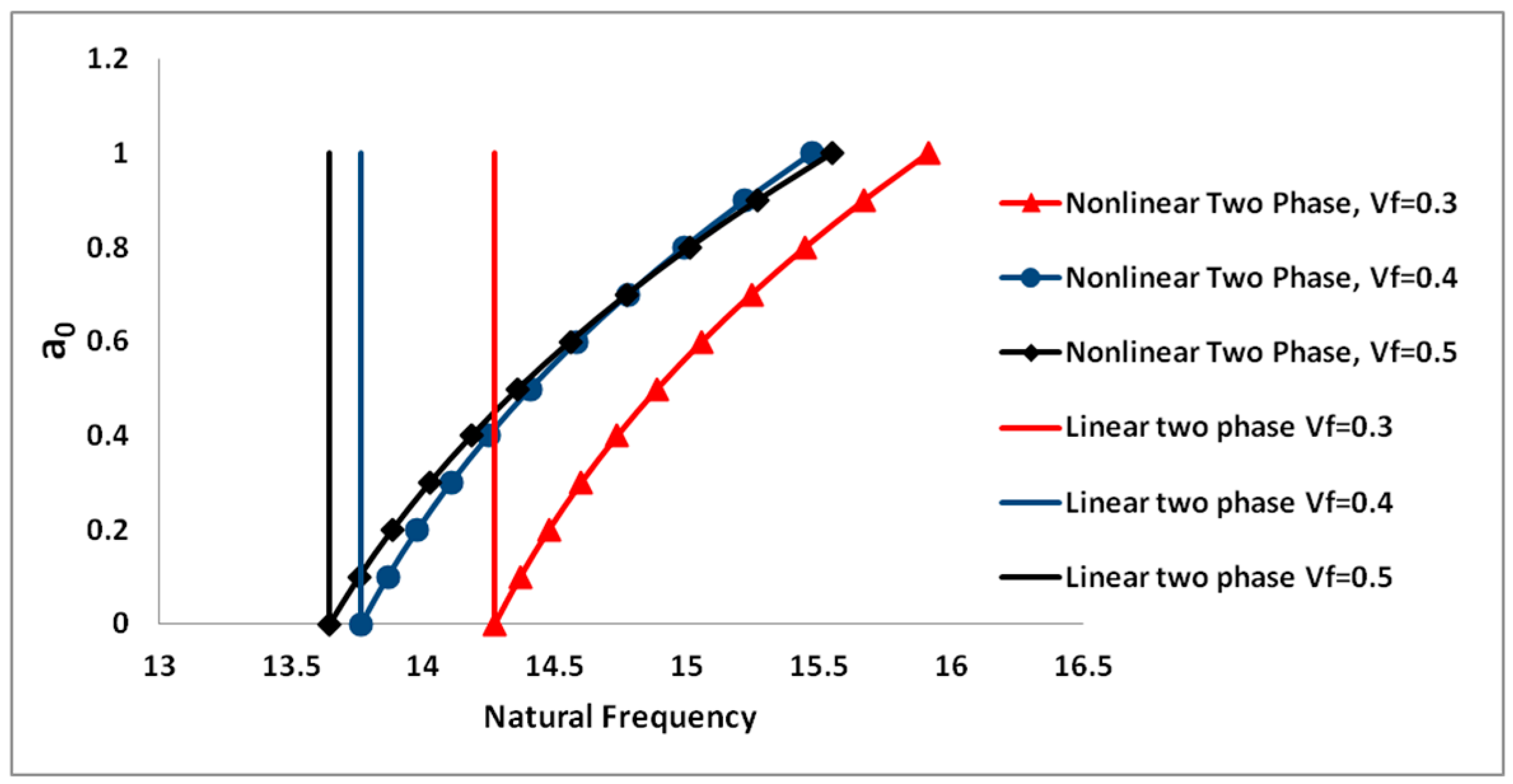
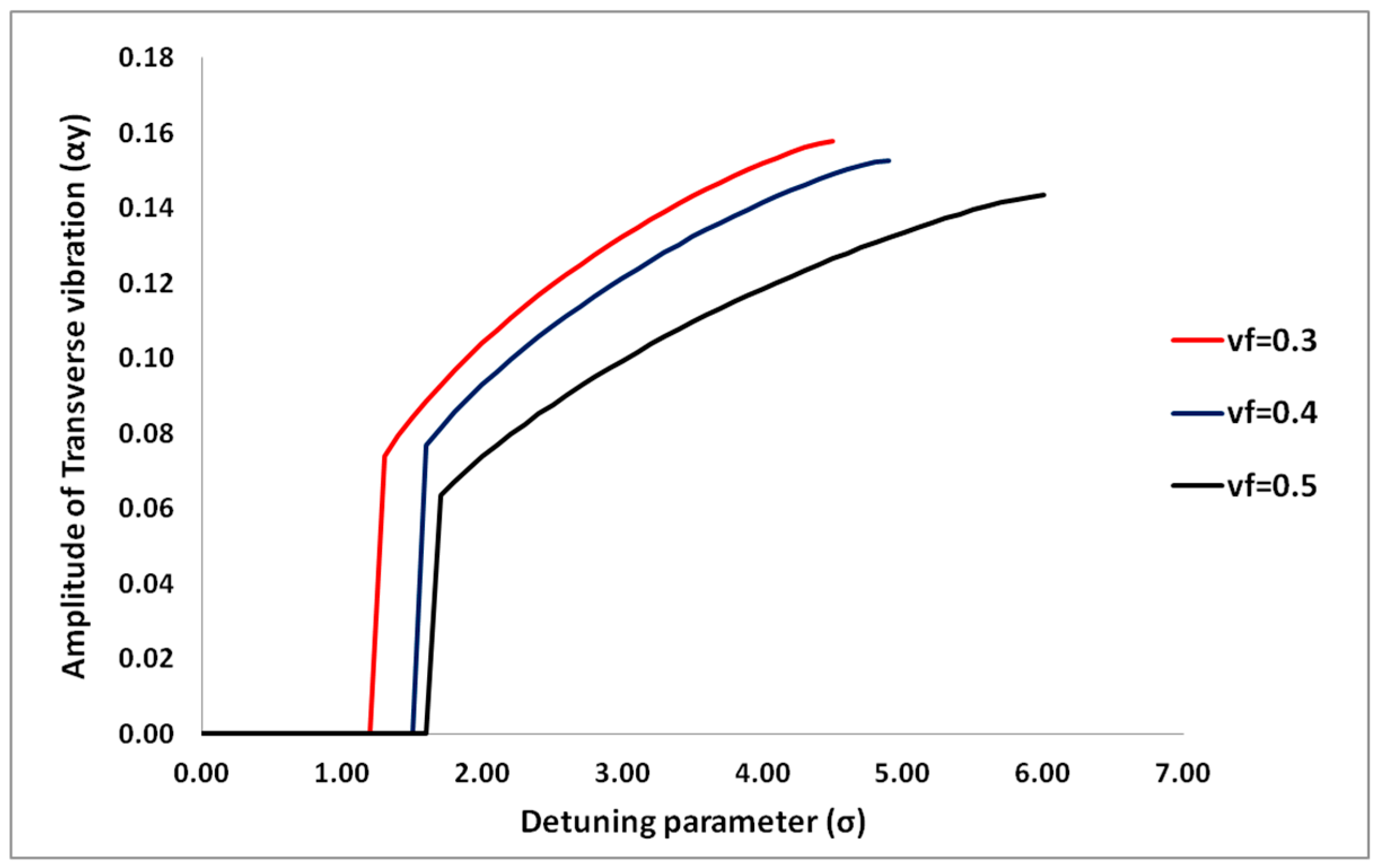
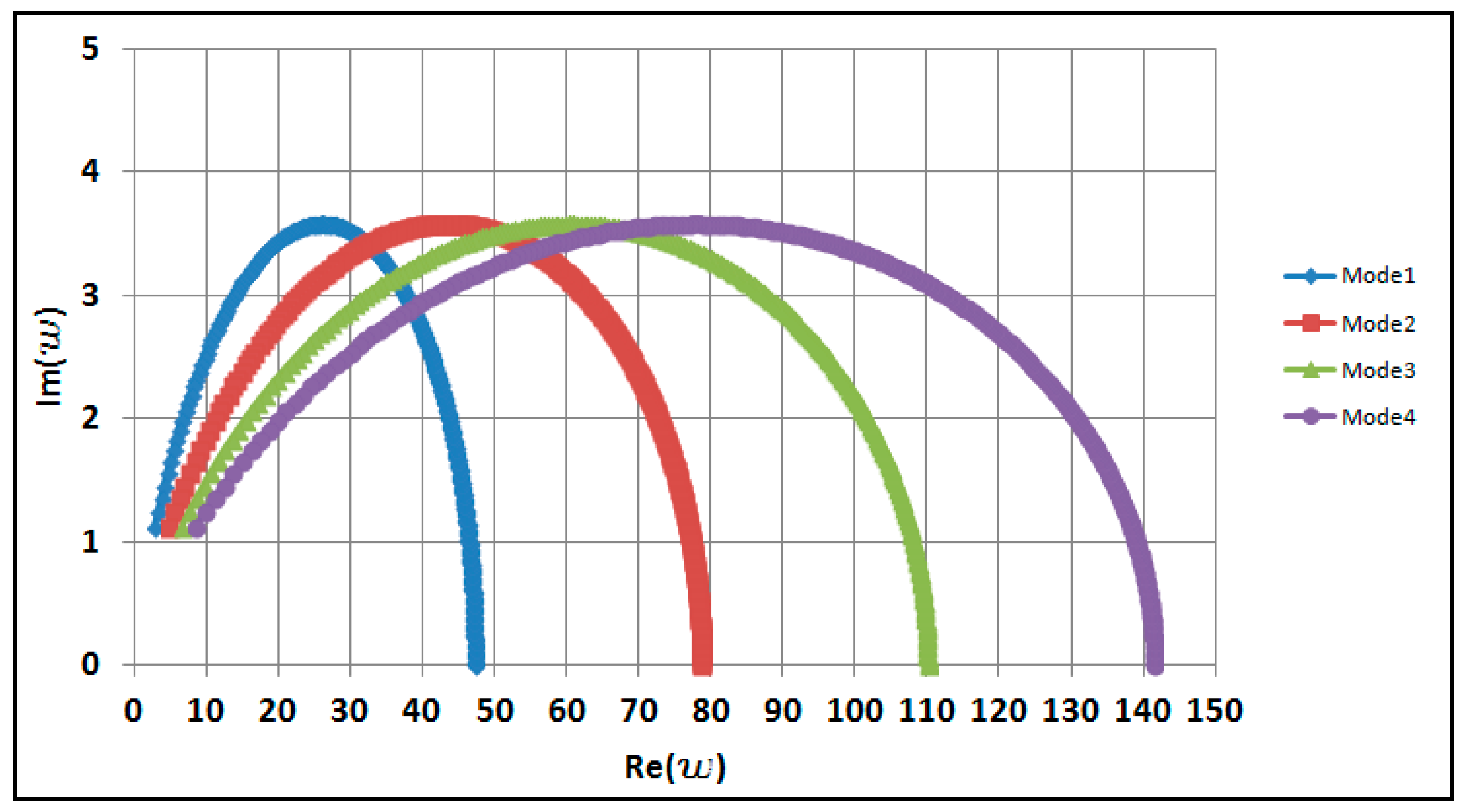
4.1. Effects of Two-Phase Flow on the Dynamic Behavior of the Pipe

The effect of two-phase flow is studied by considering the nonlinear response of the cantilever pipe as the void fraction of the two-phase flow changes. Similar to the single-phase flow, the Argand diagram of the eigen-frequencies is used to find the critical velocities of the two-phase flow for the various void fractions (0.3, 0.4, and 0.5); with the corresponding slip ratios estimated from the Chisholm empirical relations presented in Equations (26) to (29), summary of the flow parameters are presented in

Table 3. Summary of the linear two-phase solution of critical flow velocities.

Fluid	Void Fraction	$\mathit{\beta }$ Liquid	$\mathit{\beta }$ Gas	$\mathit{\Psi }$ Liquid	$\mathit{\Psi }$ Gas	Critical Mixture Velocity
						Transverse *	Axial
Two-Phase	0.3	0.19998	0.00010	0.99948	0.00052	12.505	31.634
Two-Phase	0.4	0.19997	0.00016	0.99918	0.00082	13.349	33.750
Two-Phase	0.5	0.19995	0.00024	0.99878	0.00122	14.613	36.966

* Critical mixture velocity based on Hopf bifurcation of the 2nd mode.

.

Considering a supercritical mixture velocity of 15 and book-keeping parameter (ε) of 0.1, the nonlinear frequency amplitude variations and coupled frequency response of the second mode, which is the stability-determining mode in the linear sense, are plotted for various void fractions.

It can be seen in Figure 4 that, as the void fraction increases, the natural frequency reduces. A nonlinear hardening behavior is observed in the dynamic response of the pipe for all the examined void fractions. As seen in Figure 5, as the detuning parameter is increasing, bifurcation is observed for the various void fractions examined. Also, it can be observed that the amplitude of the coupled transverse vibration is reducing as the void fraction increases.

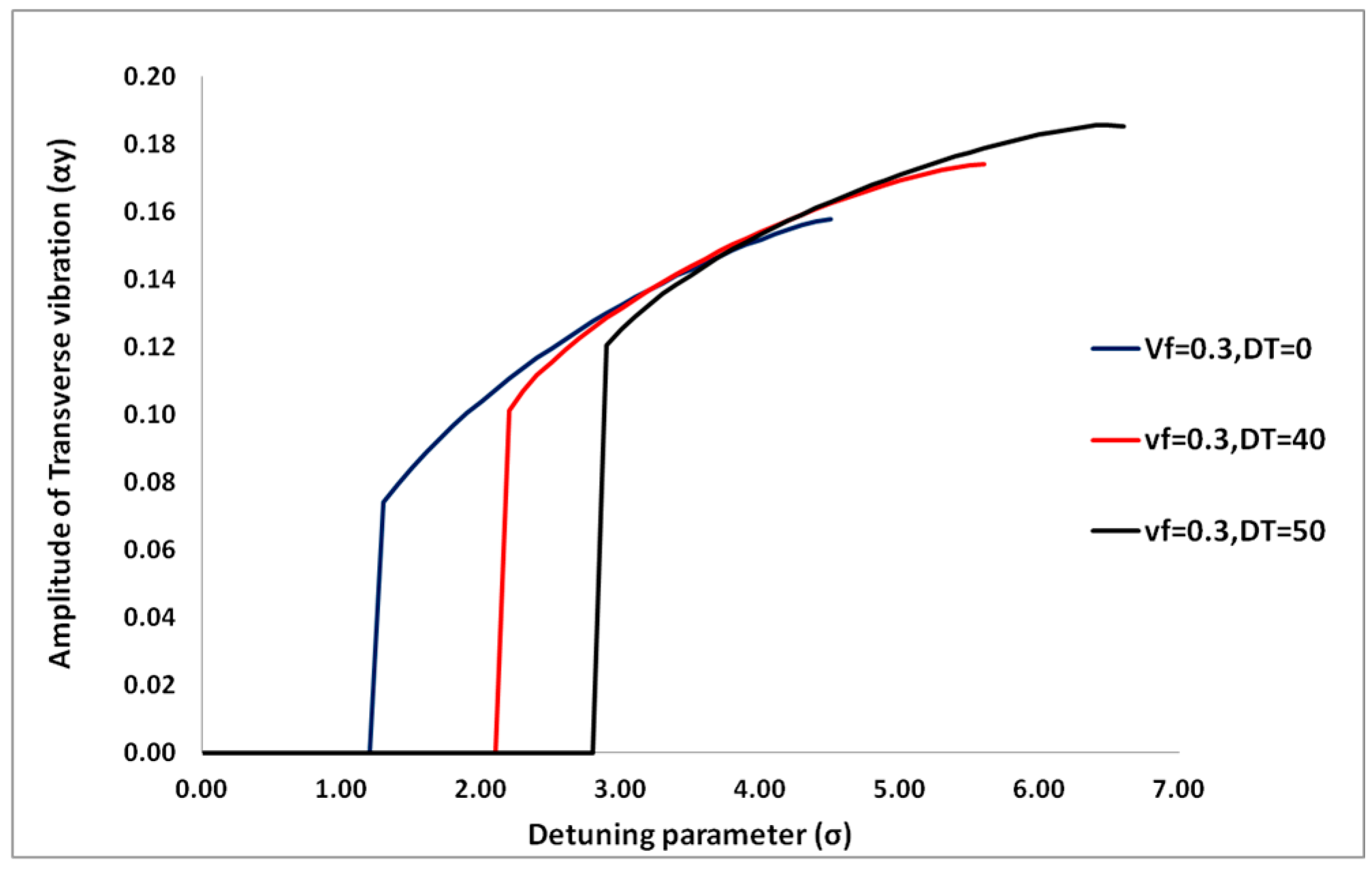
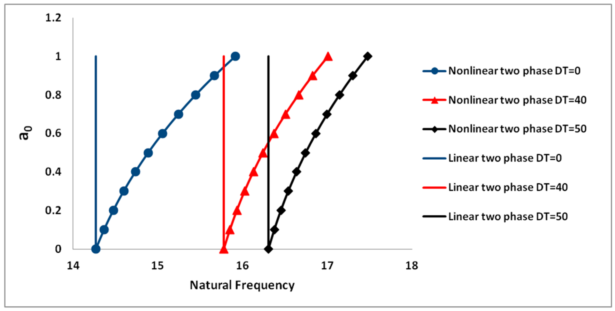
4.1.1. Effects of Temperature Difference on the Dynamic Behavior

The effect of temperature differences on a cantilever pipe conveying two-phase flow is studied by considering the nonlinear response of the cantilever pipe as the temperature difference of the two-phase flow with void fraction of 0.3 changes. Similar to the single-phase flow, the Argand diagram of the eigen-frequencies is used to find the critical velocities of the two-phase flow for the various temperature differences (0, 40, and 50); with the corresponding slip ratios estimated from the Chisholm empirical relations presented in Equations (26)–(29), summary of the flow parameters are presented in

Table 4. Summary of the linear two-phase solution of critical flow velocities for varying temperature difference.

Parameter	Void Fraction	Thermal Expansivity $\mathit{\alpha }$	Critical Mixture Velocity
			Transverse *	Axial
DT = 0	0.3	0.002	12.505	31.634
DT = 40	0.3	0.002	9.253	31.634
DT = 50	0.3	0.002	8.237	31.634

* Critical mixture velocity based on Hopf bifurcation of 2nd mode.

.

Considering a supercritical mixture velocity of 15 and book-keeping parameter (ε) of 0.1, the nonlinear frequency amplitude variations and coupled frequency response of the second mode, which is the stability-determining mode in the linear sense, is plotted for various temperature differences.

It can be seen in Figure 6 that, as the temperature difference increases, the natural frequency increases. A nonlinear hardening behavior is observed in the dynamic response of the pipe for all the examined temperature differences. As seen in Figure 7, as the detuning parameter is increasing, bifurcation is observed for the various temperature differences examined. Also, it can be observed that the increase in temperature difference did not create significant changes in the amplitude of the coupled transverse vibration.

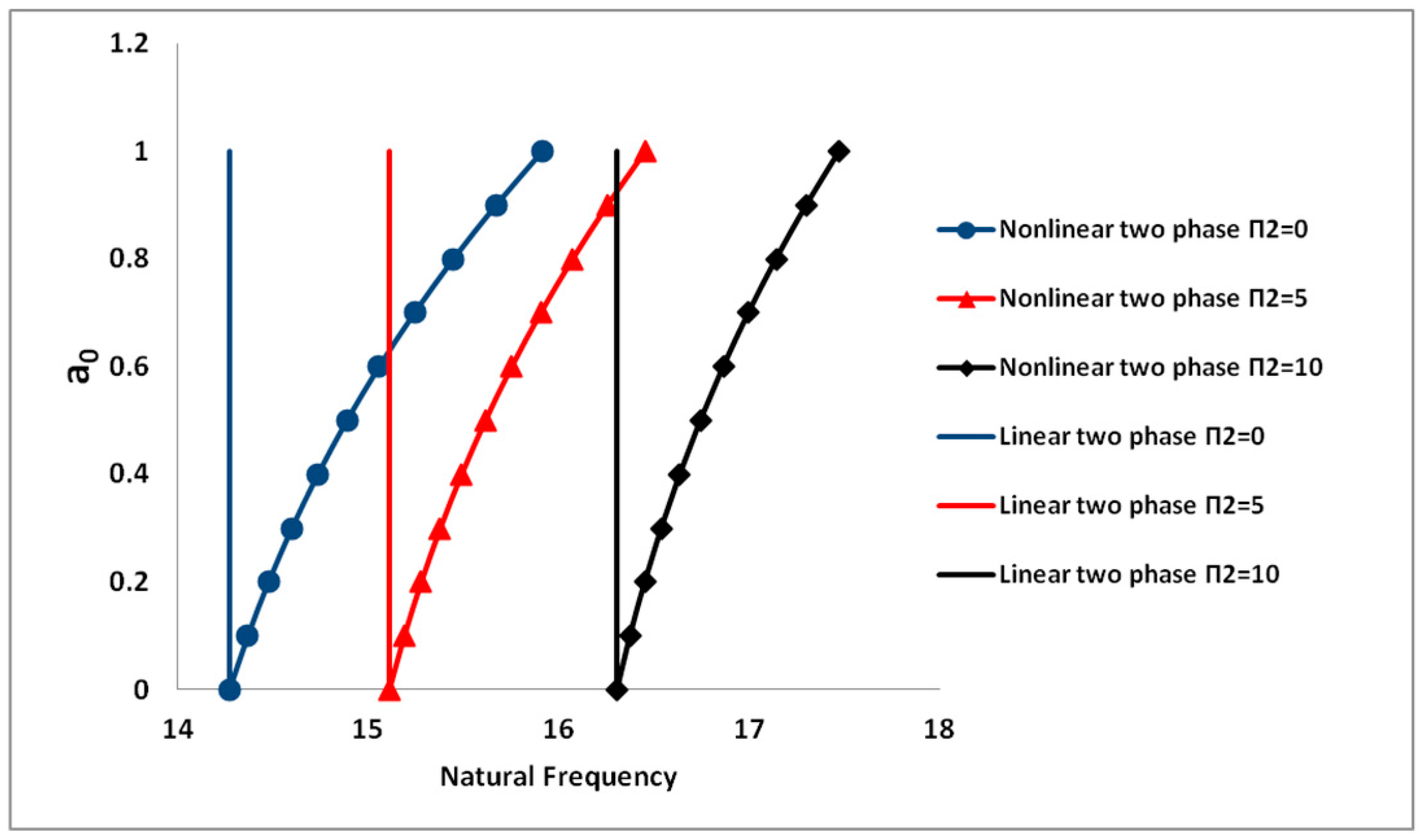
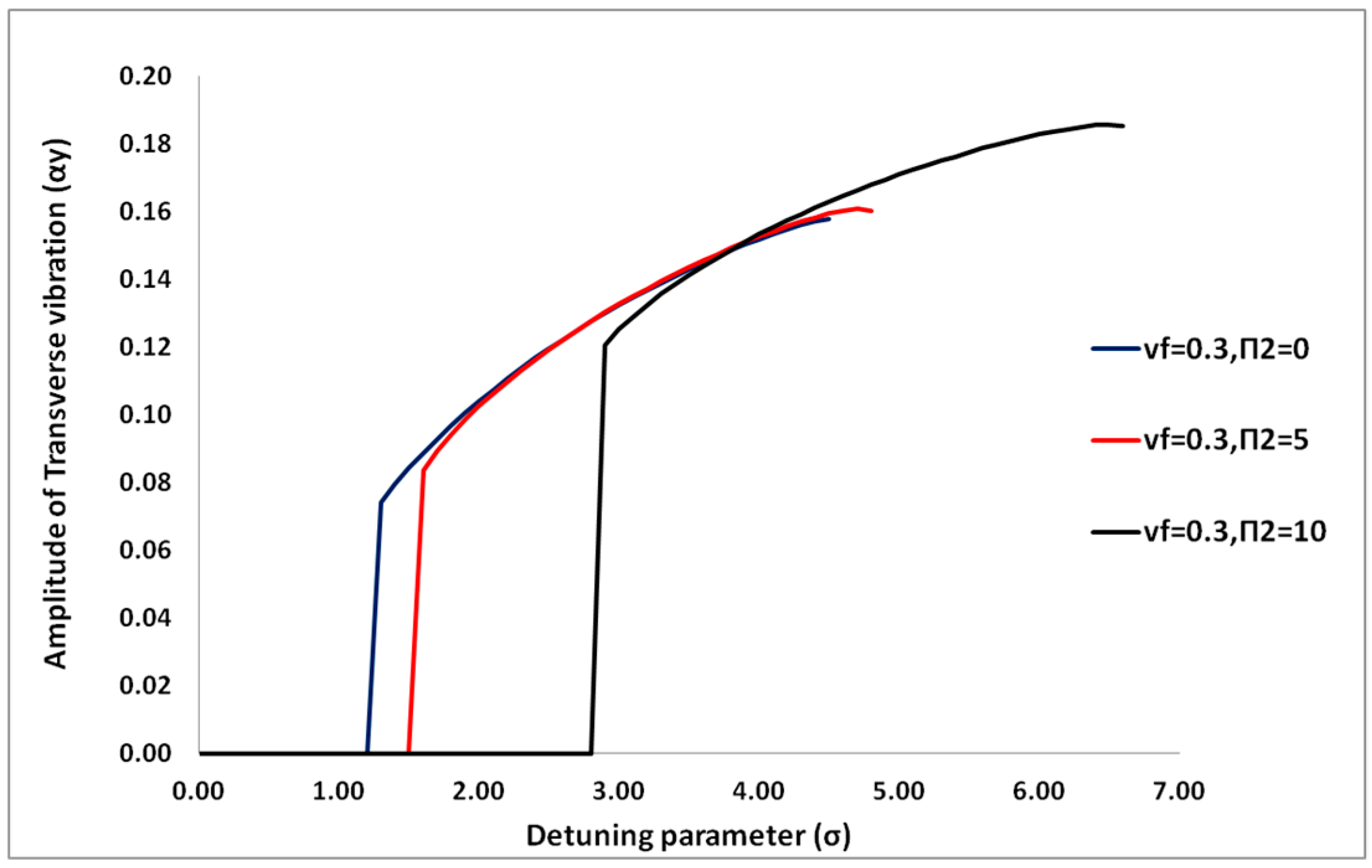
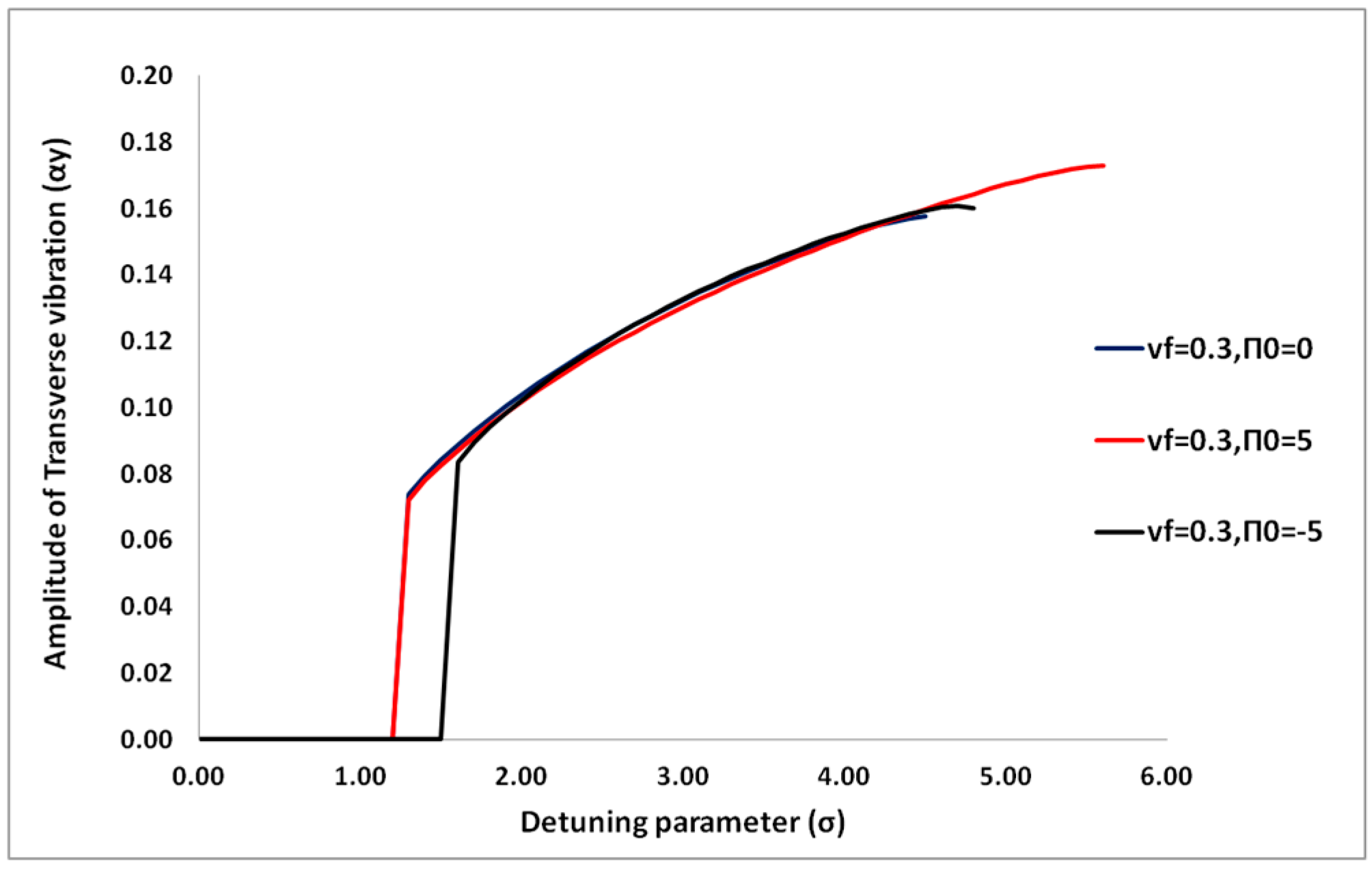
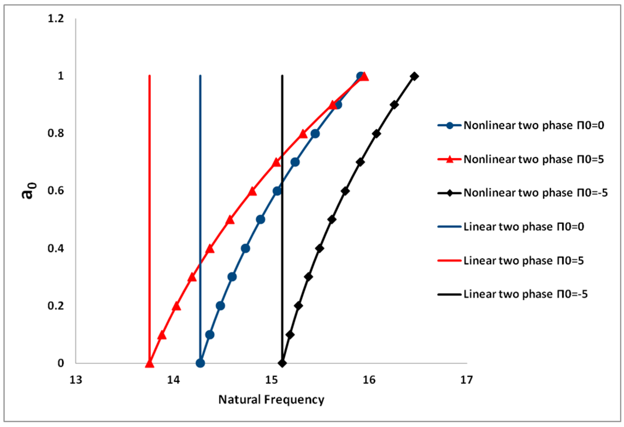
4.1.2. Effects of Flow Pressure on the Dynamic Behavior

The effect of pressurization on a cantilever pipe conveying two-phase flow is studied by considering the nonlinear response of the cantilever pipe as the pressurization of the two-phase flow with void fraction of 0.3 changes. Similar to the single-phase flow, the Argand diagram of the eigen-frequencies is used to find the critical velocities of the two-phase flow for the various pressures (0, 5, and 10); with the corresponding slip ratios estimated from the Chisholm empirical relations presented in Equations (26)–(29), summary of the flow parameters are presented in

Table 5. Summary of the linear two-phase solution of critical flow velocities for varying pressurization.

Parameter	Void Fraction	Critical Mixture Velocity
		Transverse *	Axial
$\mathit{\Pi }2=0$	0.3	12.505	31.634
$\mathit{\Pi }2=5$	0.3	10.596	31.634
$\mathit{\Pi }2=10$	0.3	8.237	31.634

* Critical mixture velocity based on Hopf bifurcation of the 2nd mode.

.

Considering a supercritical mixture velocity of 15 and book-keeping parameter (ε) of 0.1, the nonlinear frequency amplitude variations and coupled frequency response of the second mode, which is the stability-determining mode in the linear sense, is plotted for various pressures.

It can be seen in Figure 8 that, as the pressure increases, the natural frequency increases. A nonlinear hardening behavior is observed in the dynamic response of the pipe for all the examined pressures. As seen in Figure 9, as the detuning parameter is increasing, bifurcation is observed for the various pressures examined. Also, it can be observed that increasing the pressure did not create significant changes in the amplitude of the coupled transverse vibration.

4.1.3. Effects of Top Tension on the Dynamic Behavior

The effect of top tension on a cantilever pipe conveying two-phase flow is studied by considering the nonlinear response of the cantilever pipe for a situation with no top tension, a tensioning value of 5, and a compressing value of 5, with a two-phase flow and void fraction of 0.3. Similar to the single-phase flow, the Argand diagram of the eigen-frequencies is used to find the critical velocities of the two-phase flow for the various tensioning values, and the corresponding slip ratios are estimated from the Chisholm empirical relations presented in Equations (26)–(29), summary of the simulated parameters are presented in

Table 6. Summary of the linear two-phase solution of critical flow velocities for varying top tensions.

Parameter	Void Fraction	Critical Velocity
		Transverse *	Axial
$\mathit{\Pi }0=0$	0.3	12.505	31.634
$\mathit{\Pi }0=5$	0.3	14.155	31.634
$\mathit{\Pi }0=-5$	0.3	10.596	31.634

* Critical mixture velocity based on Hopf bifurcation of 2nd mode.

.

Considering a supercritical mixture velocity of 15 and book-keeping parameter (ε) of 0.1, the nonlinear frequency amplitude variations and coupled frequency response of the second mode, which is the stability-determining mode in the linear sense, is plotted for the top tensions.

It can be seen in Figure 10 that the tensioning top load reduces the natural frequency increase, while a compressing top load increases the natural frequency. A nonlinear hardening behavior is observed in the dynamic response of the pipe for all the examined cases. As seen in Figure 11, as the detuning parameter is increasing, bifurcation is observed for the various pressures examined. Also, it can be observed that the top tensions did not create significant changes in the amplitude of the coupled transverse vibration.

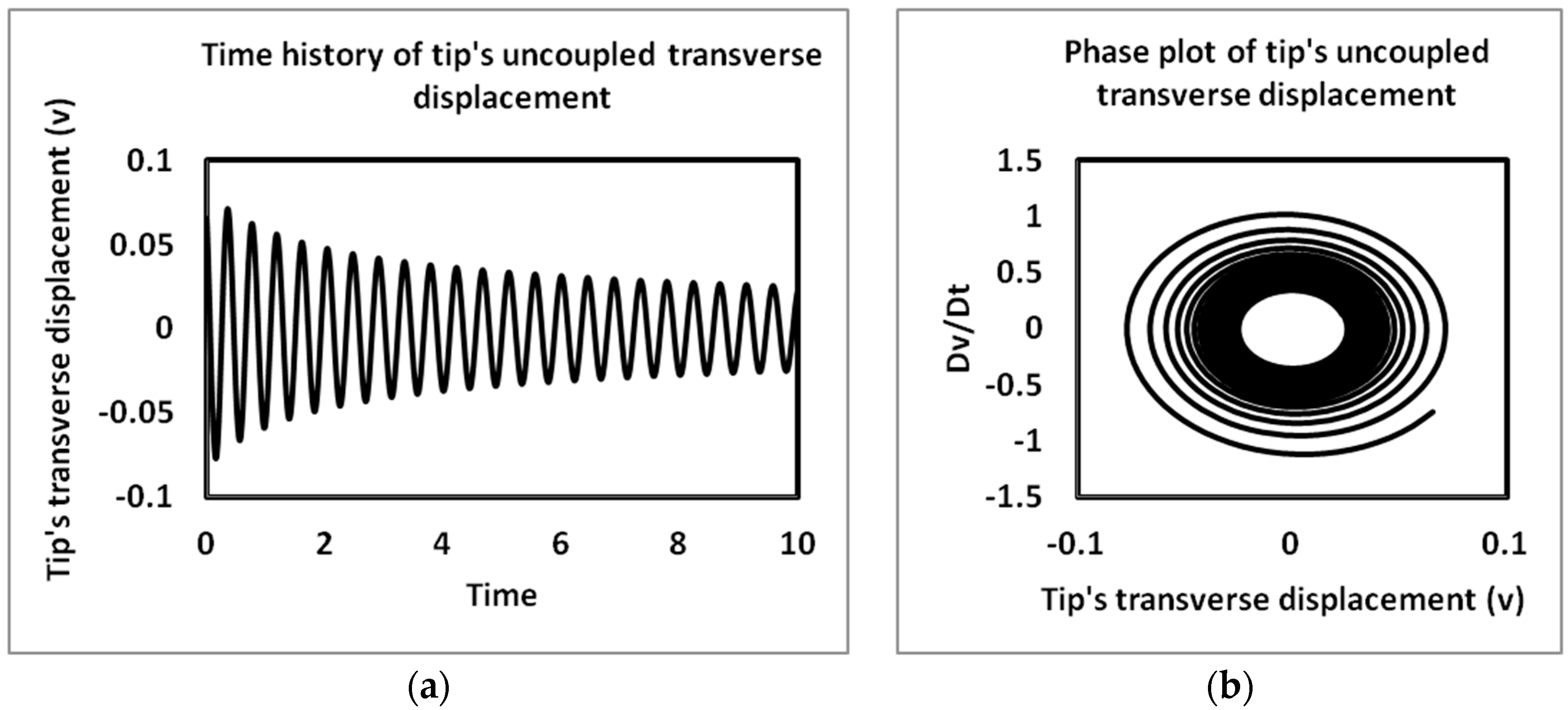
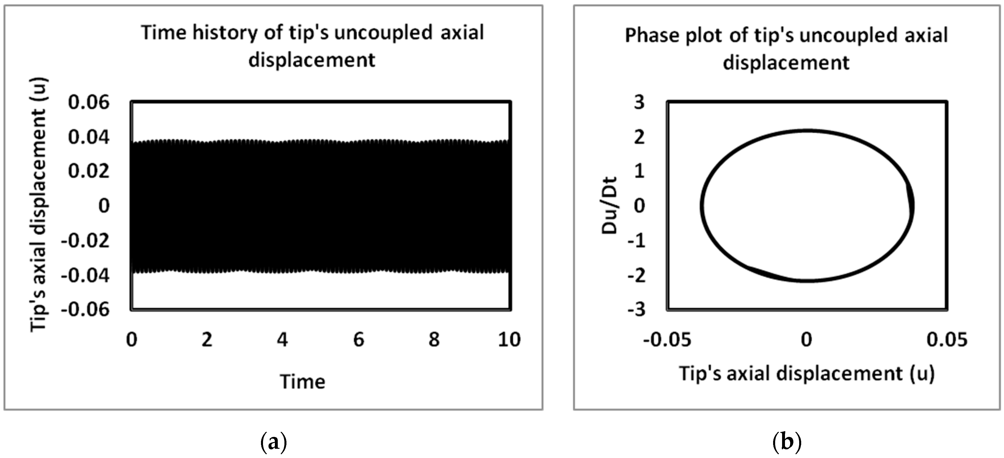
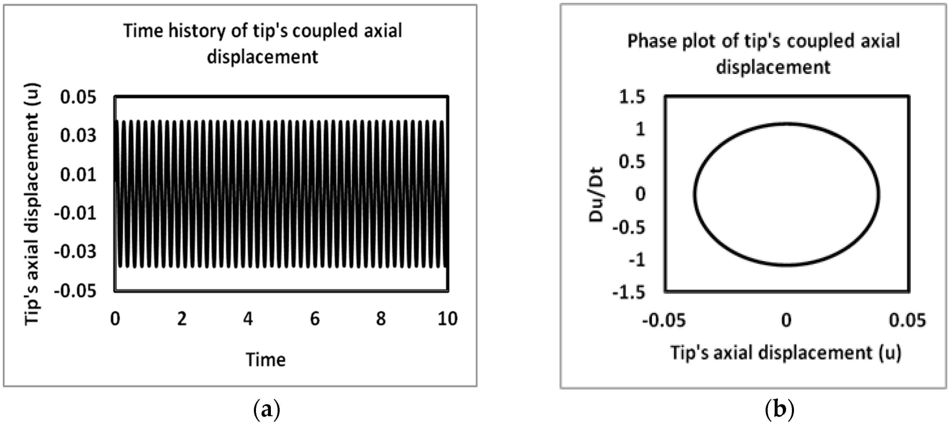
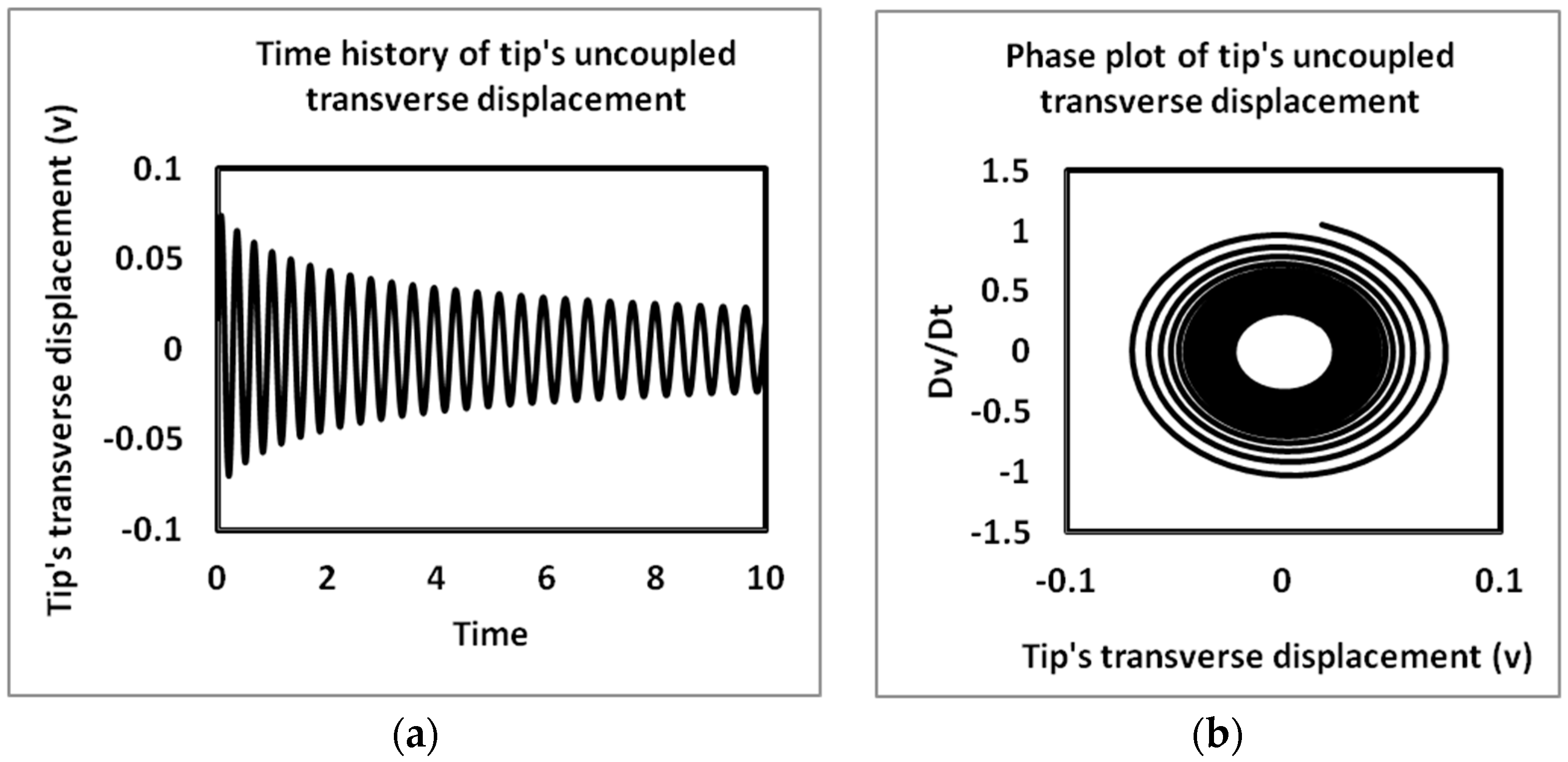
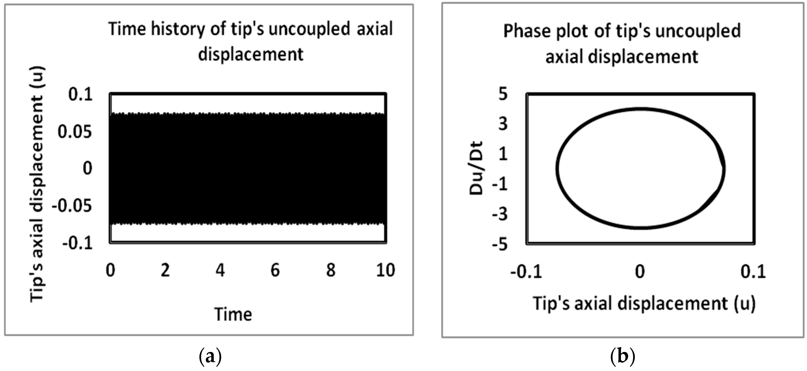
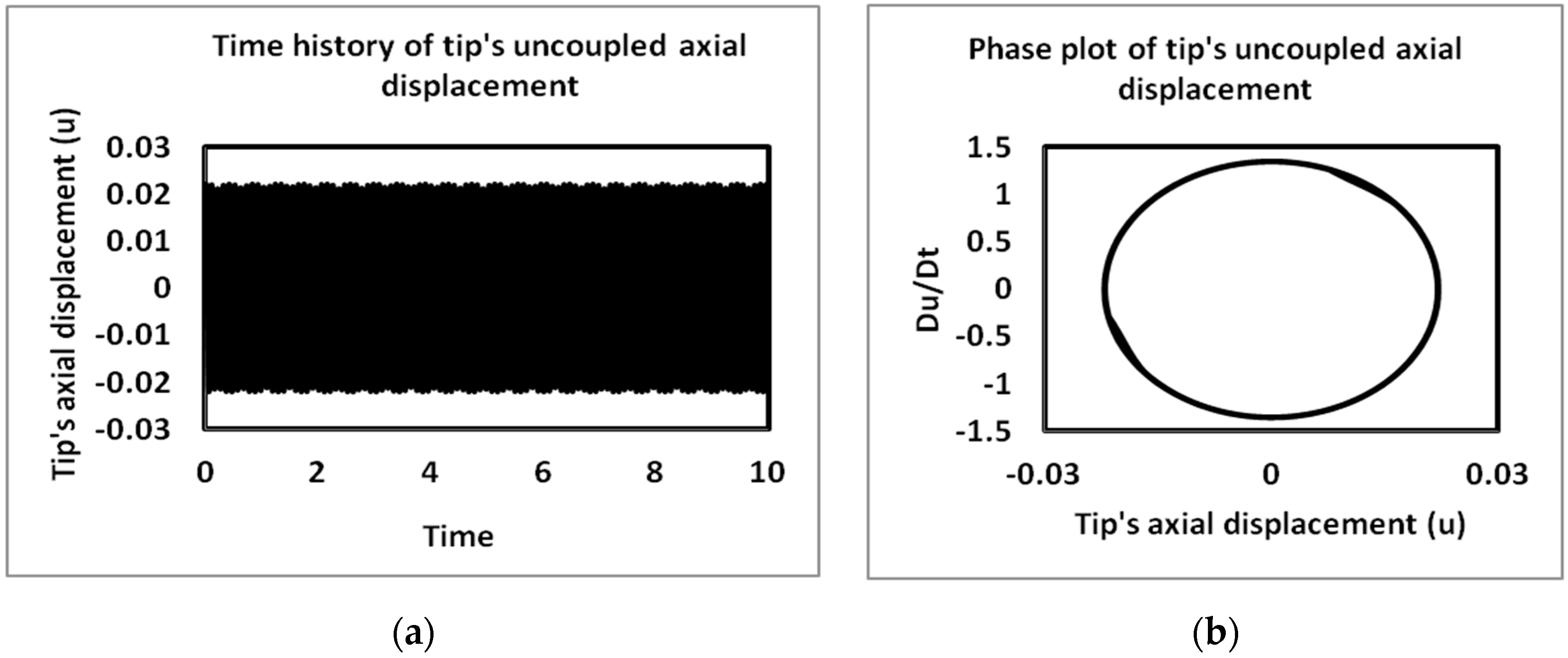
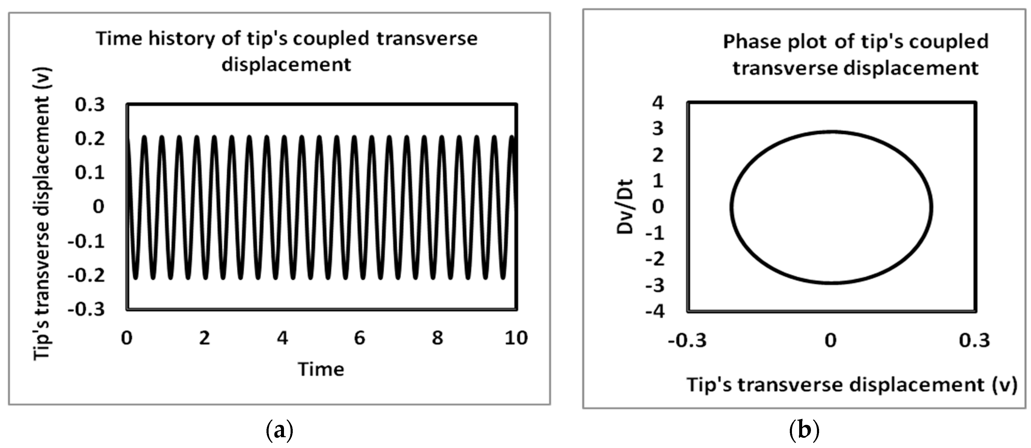
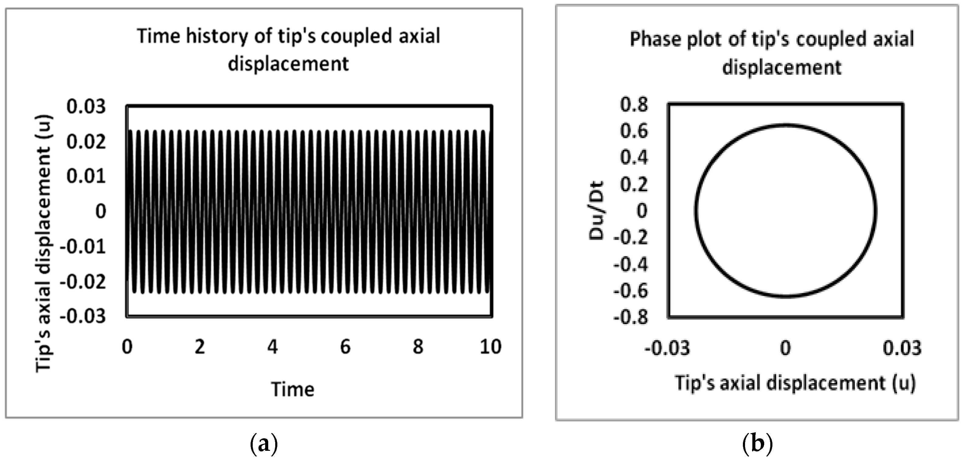
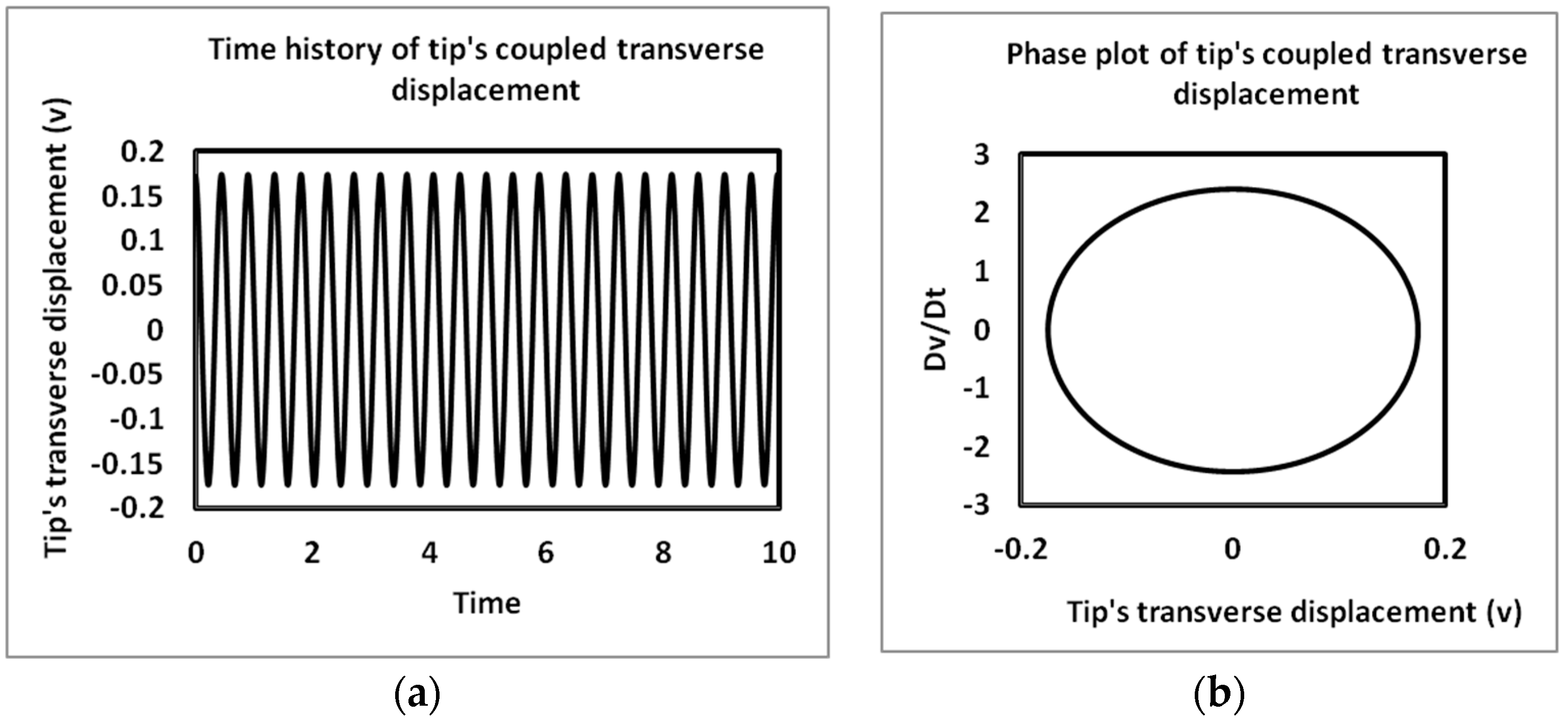
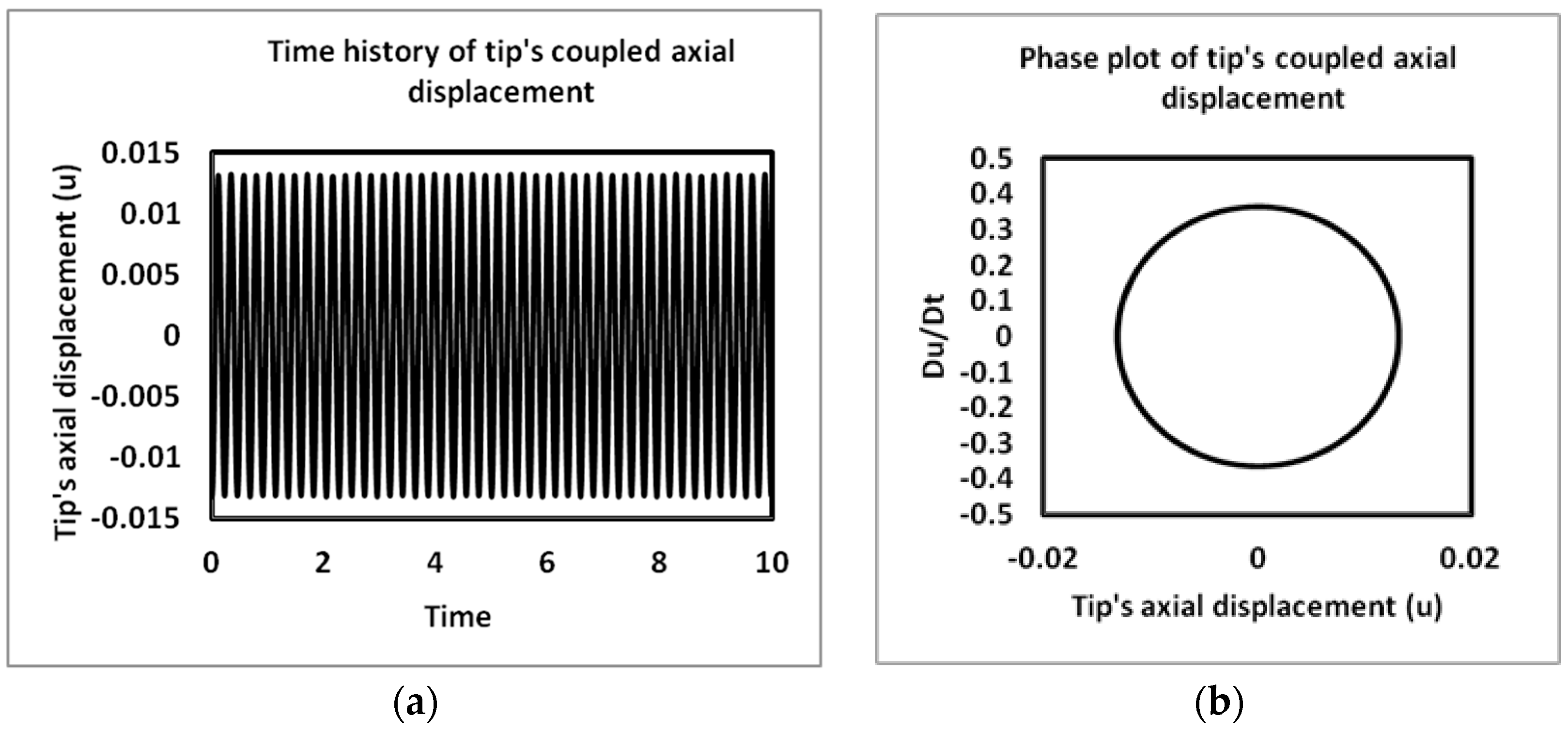
4.2. Time History and Phase Plots

Equations (83), (84), (101) and (102) are the first order approximate solutions of the transverse and axial displacement of the uncoupled and coupled vibrations of the pipe. The time trace/history and phase plots of the 2nd mode of the uncoupled and coupled vibrations are studied for various void fractions (0.3, 0.4, and 0.5) considering a post-critical flow mixture velocity of 15.

The uncoupled response of the transverse vibrations—as shown in Figure 12, Figure 13 and Figure 14 for the various void fractions—looks similar; they all reveal that the uncoupled transverse vibrations exhibit an oscillation that converges to a limit cycle with time. The initial amplitudes are greater than the amplitudes of the limit cycles; hence, a positive initial damping is observed and the amplitudes decay until they attain the limit cycles, as shown in the phase plot with a set of concentric circles inside the phase trajectories. Contrary to this, the uncoupled axial vibration—as shown in Figure 15, Figure 16 and Figure 17—is observed to exhibit uniform periodic oscillations, which traces out as a closed orbit in the phase plots. The amplitudes of the displacements are observed to reduce as the void fraction increases.

As a result of the coupling between the axial and the transverse vibration, both the coupled transverse and axial solutions—as shown in Figure 18, Figure 19, Figure 20, Figure 21, Figure 22 and Figure 23—exhibit uniform periodic oscillations, which trace out as a closed orbit in the phase plots. The amplitudes of the coupled displacements are observed to reduce as the void fraction increases.

5. Conclusions

This study examines the dynamic behavior of a cantilever pipe conveying two-phase flow. Taking into consideration the extensible theory, nonlinear equations of motion and boundary conditions were obtained using Hamilton’s principle. The equations were made to be non-dimensional so as to remove the dependence on geometric and dimensional parameters. Using the multiple-scale perturbation technique, natural frequencies, mode shapes, and first order approximate solutions of the steady state response of the pipes were obtained. From the multiple-scale assessment, it was observed that a 1:2 coupling exists between the axial and the transverse vibrations of the pipe.

The critical flow mixture velocities for various void fractions were obtained from the Argand diagram plot of the eigen-frequencies; it was observed that the critical velocity increases as the void fraction increases. The investigation on the uncoupled nonlinear dynamic behavior of the pipe as it conveys two-phase flow at a super-critical mixture velocity reveals that the system exhibits a nonlinear hardening behavior. As a result of the dynamic analysis, it has been observed that for a two-phase flow, an increase in the void fraction reduces the natural frequency and the coupled amplitude of the system. Also, an increase in temperature difference, an increase in pressure, and the presence of top tension were observed to increase the natural frequencies without a significant alteration in the coupled amplitude of the system, while compression load at the top was observed to reduce the natural frequencies without a significant change in the coupled amplitude of the system.

References

1. Miwa, S.; Mori, M.; Hibiki, T. Two-phase flow induced vibration in piping systems. Prog. Nucl. Energy 2015, 78, 270–284. [Google Scholar] [CrossRef]
2. Monette, C.; Pettigrew, M.J. Fluidelastic instability of flexible tubes subjected to two-phase internal flow. J. Fluids Struct. 2004, 19, 943–956. [Google Scholar] [CrossRef]
3. Semler, C.; Li, G.X.; Païdoussis, M.P. The Nonlinear Equations of Motion of Pipes Conveying Fluid. J. Sound Vib. 1994, 169, 577–599. [Google Scholar] [CrossRef]
4. Gregory, R.W.; Païdoussis, M.P. Unstable oscillation of tubular cantilevers conveying fluid. I. Theory. Proc. R. Soc. Lond. Ser. A Math. Phys. Sci. 1966, 293, 512–527. [Google Scholar] [CrossRef]
5. Shilling, R.; Lou, Y.K. An Experimental Study on the Dynamic Response of a Vertical Cantilever Pipe Conveying Fluid. J. Energy Resour. Technol. 1980, 102, 129–135. [Google Scholar] [CrossRef]
6. Ghayesh, M.H.; Païdoussis, M.P.; Amabili, M. Nonlinear dynamics of cantilevered extensible pipes conveying fluid. J. Sound Vib. 2013, 332, 6405–6418. [Google Scholar] [CrossRef]
7. Łuczko, J.; Czerwiński, A. Parametric vibrations of pipes induced by pulsating flows in hydraulic systems. J. Theor. Appl. Mech. 2014, 52, 719–730. [Google Scholar]
8. Païdoussis, M.P. Fluid-Structure Interactions: Slender Structures and Axial Flow; Elsevier Academic Press: London, UK, 2003. [Google Scholar]
9. Sadeghi, Y.M.; Païdoussis, M.P. Nonlinear Dynamics of Extensible Fluid-Conveying Pipes, Supported at Both Ends. J. Fluids Struct. 2009, 25, 535–543. [Google Scholar] [CrossRef]
10. Dai, L.W.H.L.; Qian, Q. Dynamics of simply supported fluid-conveying pipes with geometric imperfections. J. Fluids Struct. 2012, 29, 97–106. [Google Scholar]
11. Sinir, B.G. Bifurcation and chaos of slightly curved pipes. Math. Comput. Appl. 2010, 3, 490–502. [Google Scholar] [CrossRef]
12. Ritto, T.G.; Soize, C.; Rochinha, F.A.; Sampaio, R. Dynamic stability of a pipe conveying fluid with an uncertain computational model. J. Fluids Struct. 2014, 49, 412–426. [Google Scholar] [CrossRef]
13. Chen, L.Q.; Zhang, Y.L.; Zhang, G.C.; Ding, H. Evolution of the double-jumping in pipes conveying fluid flowing at the supercritical speed. Int. J. Non-Linear Mech. 2014, 58, 11–21. [Google Scholar] [CrossRef]
14. Yang, T.; Yang, X.; Li, Y.; Fang, B. Passive and adaptive vibration suppression of pipes conveying fluid with variable velocity. J. Vib. Control 2014, 20, 1293–1300. [Google Scholar] [CrossRef]
15. Nayfeh, A.H. Finite Amplitude Longitudinal Waves in Non-uniform Bars. J. Sound Vib. 1975, 42, 357–361. [Google Scholar] [CrossRef]
16. Nayfeh, A.H. Perturbation Methods; Wiley-VCH: Weinheim, Germany, 2004. [Google Scholar]
17. Kesimli, A.; Bağdatlı, S.M.; Çanakcı, S. Free vibrations of fluid conveying pipe with intermediate support. Res. Eng. Struct. Mater. 2016, 2, 75–87. [Google Scholar]
18. Oz, H.R.; Boyaci, H. Transverse vibrations of tensioned pipes conveying fluid with time-dependent velocity. J. Sound Vib. 2000, 236, 259–276. [Google Scholar] [CrossRef]
19. EnZ, S. Effect of asymmetric actuator and detector position on Coriolis flowmeter and measured phase shift. Flow Meas. Instrum. 2010, 21, 497–503. [Google Scholar] [CrossRef]
20. Yang, X.; Yang, T.; Jin, J. Dynamic stability of a beam-model viscoelastic pipe for conveying pulsative fluid. Acta Mech. Solida Sin. 2007, 20, 350–356. [Google Scholar] [CrossRef]
21. Oz, H.R.; Pakdemirli, M. Vibrations of an axially moving beam with time-dependent velocity. J. Sound Vib. 1999, 227, 239–257. [Google Scholar] [CrossRef]
22. Sinir, B.G.; Demir, D.D. The analysis of nonlinear vibrations of pipe conveying ideal fluid. Eur. J. Mech. B/Fluids 2015, 52, 38–44. [Google Scholar] [CrossRef]
23. Woldesemayat, M.A.; Ghajar, A.J. Comparison of void fraction correlations for different flow patterns in horizontal and upward inclined pipes. Int. J. Multiph. Flow 2007, 33, 347–370. [Google Scholar] [CrossRef]
24. Thomsen, J.J. Vibrations and Stability; Springer: Berlin, Germany, 2003. [Google Scholar]
25. Nayfeh, A.H.; Mook, D.T. Nonlinear Oscillations; John Wiley and Sons, Inc.: Hoboken, NJ, USA, 1995. [Google Scholar]
26. Sadaghi, Y.M.; Paidoussis, M.P.; Semler, C. A nonlinear model for an extensible slender flexible cylinder subjected to axial flow. J. Fluids Struct. 2005, 21, 609–627. [Google Scholar] [CrossRef]
27. Oueini, S.S.; Chin, C.M.; Nayfeh, A.H. Dynamics of Cubic Nonlinear Vibration Absorber. Nonlinear Dyn. 1999, 20, 283–295. [Google Scholar] [CrossRef]
28. Jo, H.; Yabuno, H. Amplitude reduction of parametric resonance by dynamic vibration absorber on quadratic nonlinear coupling. J. Sound Vib. 2010, 329, 2205–2217. [Google Scholar] [CrossRef]
29. Rees, E.L. General Discussion of the Roots of a Quartic Equation. Am. Math. Mon. 1922, 29, 51–55. [Google Scholar] [CrossRef]
Figure 1. System Schematics.
Mca 22 00044 g001
Figure 2. First four modes axial dimensionless complex frequency as a function of dimensionless single-phase flow velocity.
Mca 22 00044 g002
Figure 3. First four modes transverse dimensionless complex frequency as a function of dimensionless single-phase flow velocity.
Mca 22 00044 g003
Figure 4. Nonlinear frequency–amplitude variations for various void fractions.
Mca 22 00044 g004
Figure 5. Nonlinear frequency response for various void fractions.
Mca 22 00044 g005
Figure 6. Nonlinear frequency–amplitude variations for various temperature differences.
Mca 22 00044 g006
Figure 7. Nonlinear frequency response for various temperature differences.
Mca 22 00044 g007
Figure 8. Nonlinear frequency–amplitude variations for various pressures.
Mca 22 00044 g008
Figure 9. Nonlinear frequency response for various pressures.
Mca 22 00044 g009
Figure 10. Nonlinear frequency–amplitude variations for various top tensions.
Mca 22 00044 g010
Figure 11. Nonlinear frequency response for various top tensions.
Mca 22 00044 g011
Figure 12. (a) Time history and (b) phase plots of uncoupled transverse vibrations of the tip of a cantilever pipe conveying two-phase flow with void fraction of 0.3.
Mca 22 00044 g012
Figure 13. (a) Time history and (b) phase plots of uncoupled transverse vibrations of the tip of a cantilever pipe conveying two-phase flow with void fraction of 0.4.
Mca 22 00044 g013
Figure 14. (a) Time history and (b) phase plots of uncoupled transverse vibrations of the tip of a cantilever pipe conveying two-phase flow with void fraction of 0.5.
Mca 22 00044 g014
Figure 15. (a) Time history and (b) phase plots of uncoupled axial vibrations of the tip of a cantilever pipe conveying two-phase flow with void fraction of 0.3.
Mca 22 00044 g015
Figure 16. (a) Time history and (b) phase plots of uncoupled axial vibrations of the tip of a cantilever pipe conveying two-phase flow with void fraction of 0.4.
Mca 22 00044 g016
Figure 17. (a) Time history and (b) phase plots of uncoupled axial vibrations of the tip of a cantilever pipe conveying two-phase flow with void fraction of 0.5.
Mca 22 00044 g017
Figure 18. (a) Time history and (b) phase plots of coupled transverse vibrations of the tip of a cantilever pipe conveying two-phase flow with void fraction of 0.3, σ of 2.0.
Mca 22 00044 g018
Figure 19. (a) Time history and (b) phase plots of coupled axial vibrations of the tip of a cantilever pipe conveying two-phase flow with void fraction of 0.3, σ of 2.0.
Mca 22 00044 g019
Figure 20. (a) Time history and (b) phase plots of coupled transverse vibrations of the tip of a cantilever pipe conveying two-phase flow with void fraction of 0.4, σ of 2.0.
Mca 22 00044 g020
Figure 21. (a) Time history and (b) phase plots of coupled axial vibrations of the tip of a cantilever pipe conveying two-phase flow with void fraction of 0.4, σ of 2.0.
Mca 22 00044 g021
Figure 22. (a) Time history and (b) phase plots of coupled transverse vibrations of the tip of a cantilever pipe conveying two-phase flow with void fraction of 0.5, σ of 2.0.
Mca 22 00044 g022
Figure 23. (a) Time history and (b) phase plots of coupled axial vibrations of the tip of a cantilever pipe conveying two-phase flow with void fraction of 0.5, σ of 2.0.
Mca 22 00044 g023