Novel Spreadsheet Direct Method for Optimal Control Problems


ExcelWorks LLC, Sharon, MA 02067, USA
Math. Comput. Appl. 2018, 23(1), 6; https://doi.org/10.3390/mca23010006
Submission received: 26 December 2017
/
Revised: 22 January 2018
/
Accepted: 23 January 2018
/
Published: 25 January 2018
(This article belongs to the Special Issue Optimization in Control Applications)
Abstract
:We devise a simple yet highly effective technique for solving general optimal control problems in Excel spreadsheets. The technique exploits Excel’s native nonlinear programming (NLP) Solver Command, in conjunction with two calculus worksheet functions, namely, an initial value problem solver and a discrete data integrator, in a direct solution paradigm adapted to the spreadsheet. The technique is tested on several highly nonlinear constrained multivariable control problems with remarkable results in terms of reliability, consistency with pseudo-spectral reported answers, and computing times in the order of seconds. The technique requires no more than defining a few analogous formulas to the problem mathematical equations using basic spreadsheet operations, and no programming skills are needed. It introduces an alternative, simpler tool for solving optimal control problems in social and natural science disciplines.
1. Introduction
Optimal control problems are commonly encountered in engineering and life sciences, as well as social studies such as economics and finance [1,2,3]. An optimal control problem is typically concerned with finding optimal control functions (or policies) that achieve optimal trajectories for a set of controlled differential state variables. The optimal trajectories are decided by a constrained dynamical optimization problem, such that a cost functional is minimized or maximized subject to certain constraints on state variables and the control functions. Mathematically, an optimal control problem may be stated as follows:
Find the control functions and the corresponding state variables which minimize (or maximize) the functional
subject to
with initial conditions
and optional final conditions and bounds
In the formulation (1)–(5), the generally nonlinear H and G are scalar functions, whereas F, Q, and S are vector-valued functions. Typically, either H or Q are specified but not both in the same problem. Common forms of Q and S are and , respectively. We have chosen not to include and in the formulation because a higher-order explicit differential equation system can be restated as a first-order system via variable substitution. The matrix M in (2) offers an optional coupling of the states’ temporal derivatives by a mass matrix which may be singular. If M is singular, the equation system (2) is differential algebraic, or DAE. For uncoupled derivatives, M is the identity matrix which can be omitted. Furthermore, T, which denotes the final time, may be fixed or free.
Numerical solution strategies of (1)–(5) fall into one of two approaches: an indirect method, where Pontryagin’s minimum principle is employed to transform the problem into an augmented Hamiltonian system requiring the solution of a boundary value problem [4]; and a direct method, where the original system’s variables are approximated by parameterized appropriate functions which, in turn, reduce the problem into a finite-dimensional nonlinear programming problem [5]. Direct methods can be further classified as full or partial parametrization methods. In the latter, only the controls are parametrized, wherein the inner initial value problem (IVP) (2)–(3) is treated as a separate dependent problem that must be solved repeatedly by the outer nonlinear programming (NLP) algorithm [6].
Except for the most trivial cases, optimal control problems can be difficult to solve, particularly for those who are not inclined towards programming and numerical methods. Despite advances in software programs, it remains a nontrivial task to utilize a standard package such as MATLAB to solve optimal control problems. The student must have sufficient programming skill, as well as a good understanding of the general structure of the solution algorithm and the various solvers required to implement it [7].
In this article, we present a systematic technique for solving optimal control problems in a spreadsheet, modeled on partial parametrization direct methods. The technique is made possible, on the one hand, by algorithmic advances [8,9] which enabled the introduction of mathematically pure calculus worksheet functions to the spreadsheet [10,11]. A pure calculus function is evaluated as a standard built-in math function; however, it accepts, via input parameters, formulas representing a problem model and outputs a formatted solution result. Specifically, we make use of two calculus functions described in Appendix A: an IVP solver, based on an implicit RADUA5 algorithm with adaptive step control [12], which we employ for solving the inner IVP (2)–(3); and a discrete data integrator, based on cubic spline approximations [13], which we employ to approximate the cost index (1). On the other hand, Excel spreadsheets include a powerful NLP Solver Command based on the Generalized Reduced Gradient Method (GRG) [14] which is compatible with the calculus functions. We devise a direct control–parametrization method based on employing the calculus functions with the NLP Solver in a dynamical optimization paradigm for the solution of (1)–(5).
Attempts to solve optimal control problems in spreadsheets are not new; however, to the best of our knowledge, no prior work has presented a practical direct spreadsheet method aimed at solving the general nonlinear multidimensional optimal control problem (1)–(5). The chief reason is that prior approaches utilized the spreadsheet explicitly as the computational grid for the discretization and solution of the underlining IVP. This limits the practical scope to rather simple problems that can be easily discretized with an explicit differencing scheme suitable for the spreadsheet. For example, Weber [15] demonstrated a direct approach to solving control problems in resource economics involving simple one-dimensional IVPs, and direct summation of discrete values for the cost index. Nævdal [16] demonstrated a basic implementation of the indirect method, with the aid of Visual Basic for Applications (VBA) programming, to solve one-dimensional optimal control problems. The method utilized Excel’s Solver in conjunction with an explicit difference scheme and a shooting algorithm to solve the resulting boundary value problem. While Nævdal’s work provides educational insights into the mechanics of the indirect solution method, its detail-intensive implementation makes it impractical to use or extend to higher dimensions or nonlinear stiff systems requiring adaptive implicit schemes. Our devised direct spreadsheet method, on the other hand, differs fundamentally from prior work, in that the algorithmic implementation for solving the IVP, and integrating the cost index, has been decoupled from the spreadsheet grid and encapsulated in pure spreadsheet solver functions suitable for seamless integration with the NLP Solver. The design of the solver functions, described in Section 2, permits utilization of fully implicit and adaptive algorithms which make the method applicable to a general class of nonlinear multivariable optimal control problems. Furthermore, by encapsulating the tedious implementation details in standard pure math functions with a clear divide between input and output, the method is applicable with little more than basic spreadsheet knowledge, and without any programming skills. As demonstrated in Section 3, results obtained on several highly nonlinear problems are remarkable, in terms of both the reliability and the computing time in the order of seconds. The devised method extends the utility of the spreadsheet beyond what has been practical or even feasible before.
The remainder of this paper is organized as follows: In the next section, we describe the basic steps required to model and solve an optimal control problem using the adapted direct method technique. In Section 3, we demonstrate the technique for solving four different control problems reproduced from Elnagar and Kazemi [17] who used a pseudo-spectral direct method. The problems include:
- A bang–bang control problem.
- A highly nonlinear and coupled system.
- A minimum swing container transfer problem involving multiple controls and constraints.
- A minimum time orbit transfer control problem with free end time.
Section 4 provides some practical tips for applying the technique, followed by conclusions in Section 5. Appendix A includes a description for the IVP solver, IVSOLVE, and the discrete data integrator functions, QUADXY, both of which are essential for the technique. We also remark that our main focus in this first article is to introduce and illustrate the spreadsheet direct solution method rather than formulate or study any specific optimal control problem. As such, we start from a mathematical statement of a given problem and present a feasible solution obtained by the method with relevant comparisons to the reported result in [17].
2. Spreadsheet-Adapted Direct Solution Method
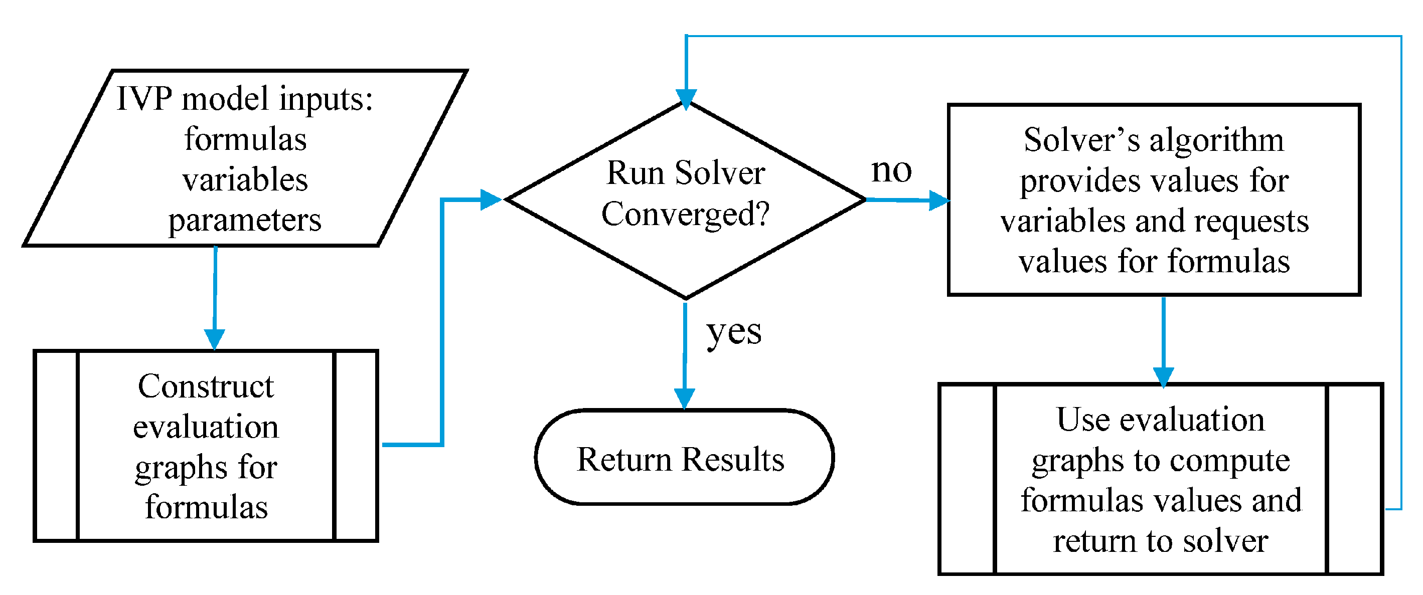
The main enabling elements of the devised method are, in addition to the NLP Solver, the IVP solver function, IVSOLVE, and the discrete data integrator, QUADXY. The IVSOLVE spreadsheet function, described in Appendix A.1, is designed according to the flowchart of Figure 1, wherein a suitable highly accurate algorithm, such as RADUA5 [12], is fully shielded with a strict divide between the IVP model input and the output solution results. The model input is represented by formulas that are direct analogues to the IVP mathematical equations, and the output solution results are displayed in a formatted tabular array of elective resolution which is easily adjusted to yield an accurate integration of a dependent cost index. By design, IVSOLVE is a pure function which does not modify its input but merely computes and displays the solution in its allocated spreadsheet array. QUADXY, on the other hand, follows a standard spreadsheet User Defined Function (UDF) implementation to integrate a vector of ordered points, . QUADXY performs the integration with the aid of cubic splines fit to the data. Under the assumption that the discrete data describe a smooth curve, the computed integral is generally quite accurate and can be further improved by supplying optional slopes at the end points of the curve when they are known or can be estimated. Likewise, QUADXY is also a pure function which does not modify its inputs.
Below, we describe the general steps for employing IVSOLVE and QUADXY with the NLP Solver for solving the optimal control problem (1)–(5). Some of these steps may or may not be required for a given problem. To simplify the discussion, we shall assume a single control function, u(t). Extension to multiple controls is straightforward and is demonstrated by the examples. In practice, there are three systematic tasks:
Task 1
The first step is to obtain, with the IVP solver function, IVSOLVE, an initial solution for the underlining IVP (2)–(3) using an appropriately parametrized formula for the control function and initial guesses for the unknown parameters. A continuous control function can be parametrized, for example, by a third-order polynomial with unknown coefficients, such as ‘=c_0+c_1*t+c_2*t^2+c_3*t^3’. On the other hand, a discontinuous control function can be modeled using the standard IF statement in Excel. For example, a two-stage, constant controller can be defined as follows: ‘=IF(t<=ts,value1,value2)’. Here ts, value1, and value2 are unknown parameters that would be assigned initial guesses.
Task 2
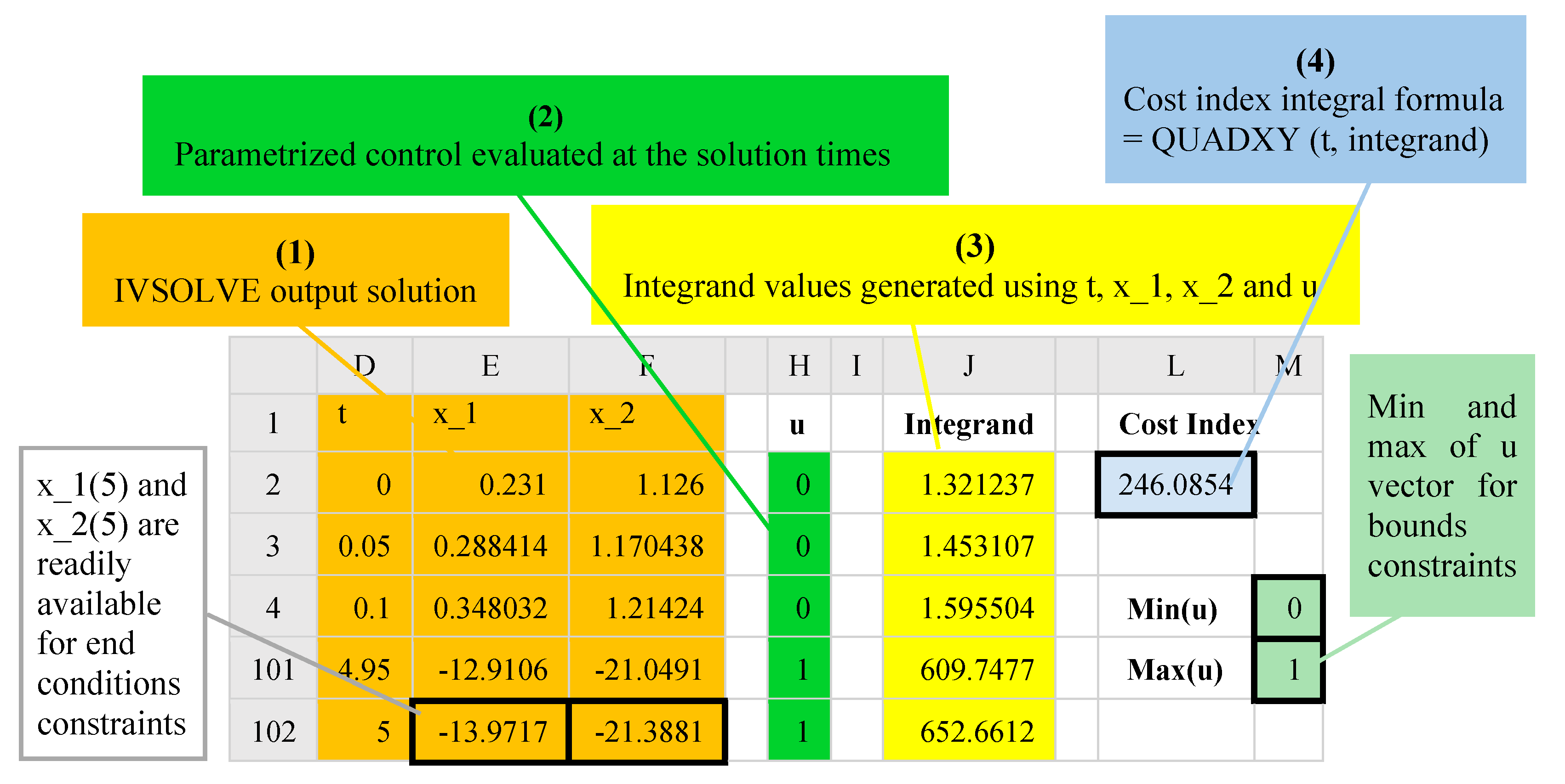
In the second task we define an analogous objective formula for the cost functional (1). Our strategy is to integrate, using QUADXY, a sampled vector of the integrand expression in (1) using the solution values obtained in Task 1. To accomplish this, in a new column, we generate values for the parametrized control formula evaluated at the solution’s output times and, in a second column, we generate values for the integrand expression, using the solution’s state variables and generated control values as needed. Both the control and integrand columns are easily generated using the AutoFill feature of Excel. To define an analogous objective formula for the cost index (1), we employ the discrete data integrator function, QUADXY, to integrate the generated integrand data column versus the solution’s output times column. The ordered steps needed to define the objective formula are summarized in Figure 2.
Task 3
The last task is to configure and run Excel’s NLP Solver. The NLP Solver can be configured to minimize or maximize an objective formula by changing design variables, subject to defined constraints. The design variables are the unknown parameters which are assigned initial guesses in Task 1. The constraints (4) and (5) are added directly in the Solver’s dialog. Simple equality end conditions on state variables are added by referencing the corresponding cells in the solution output as illustrated in Figure 2. Bound constraints on state variables or controls are easily imposed with the aid of Excel’s MAXA() and MINA() math functions which compute the maximum and minimum values of a vector. Concrete examples are presented in the next section.
How It Works
Key to the successful operation of the adapted direct solution method are two attributes: the purity of the IVP solver function, and the Automatic Calculation Mode of the spreadsheet. As described earlier, the IVSOLVE function does not modify its inputs, and the authority to modify the inputs to IVSOLVE via changes to the decision parameter vector is confined to the outer NLP Solver command. On the other hand, the spreadsheet maintains a dependency hierarchy, and updates all information whenever a change occurs. Any modification to the design parameters by the outer NLP Solver triggers reevaluation of the inner IVSOLVE solution, the dependent control and integrand columns, the objective, and any constraint formulas in the proper order. The NLP Solver always receives up-to-date values for the objective and constraints whenever it alters the design variables’ values.
3. Illustrative Examples
In this section, we apply the spreadsheet method to solve four optimal control problems reproduced from Elnagar and Kazemi [17], who used a pseudo-spectral high order Chebyshev approximation scheme in conjunction with the general-purpose sequential programming software package NLPQL. Relevant comparisons with reported results in [17] are included. The examples are representative of various types of optimal control problems and intended to serve as a template as well as validation for the effectiveness of the devised spreadsheet method. We recommend that the reader review Appendix A prior to reading the examples. Also, some basic familiarity with the spreadsheet operation is assumed, including naming variables, defining formulas, and running the NLP Solver command.
3.1. A Bang–Bang Control Problem
The first example describes a bang–bang (two-stage) control problem. The mathematical problem is stated as follows:
Minimize
subject to
3.1.1. Spreadsheet Model
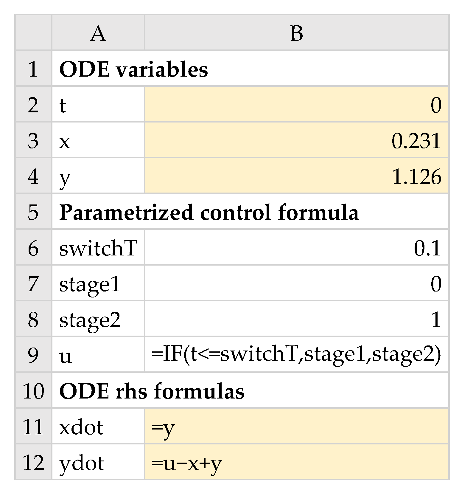
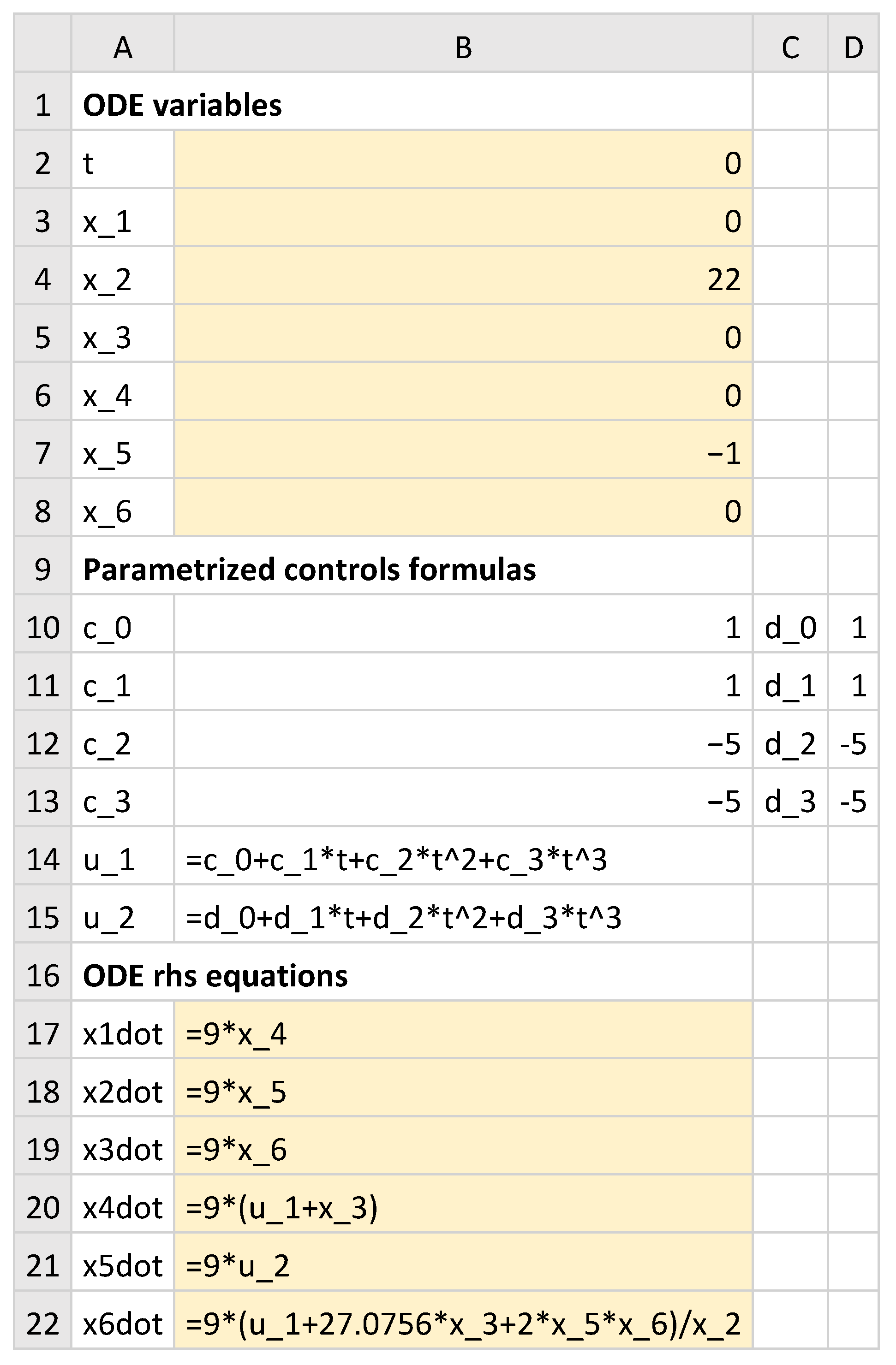
Working with named variables with adjacent labels shown in Column A of Figure 3, we parametrized the two-stage control function, u(t), using a standard IF() statement, as shown in B9. The unknown parameters switchT, stage1, and stage2 were assigned the initial guess values 0.1, 0, and 1. The right-hand sides of the IVP differential Equations (7) and (8) were represented by the equivalent formulas B11 and B12, and the initial conditions (9) were assigned to the variables x and y in B3 and B4. The colored ranges in Figure 3 represent the model input required to obtain the initial solution for the IVP (7)–(9) using the IVSOLVE function. The initial solution was obtained by evaluating the formula
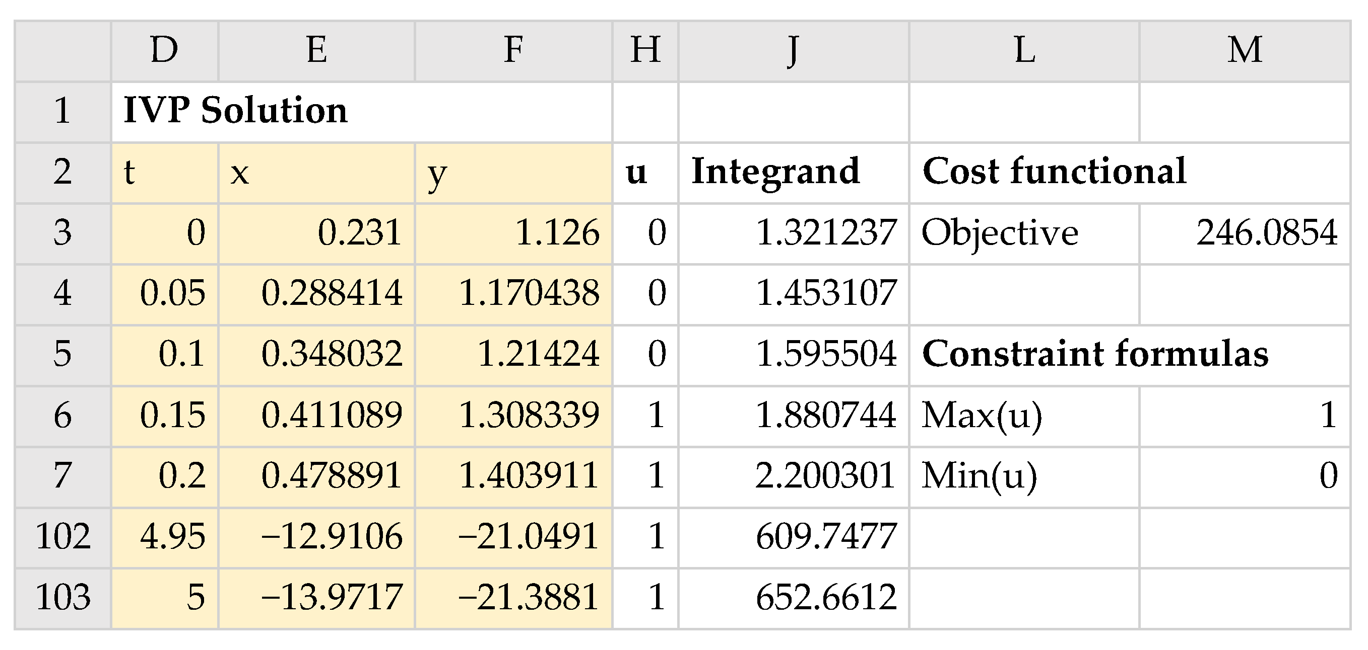
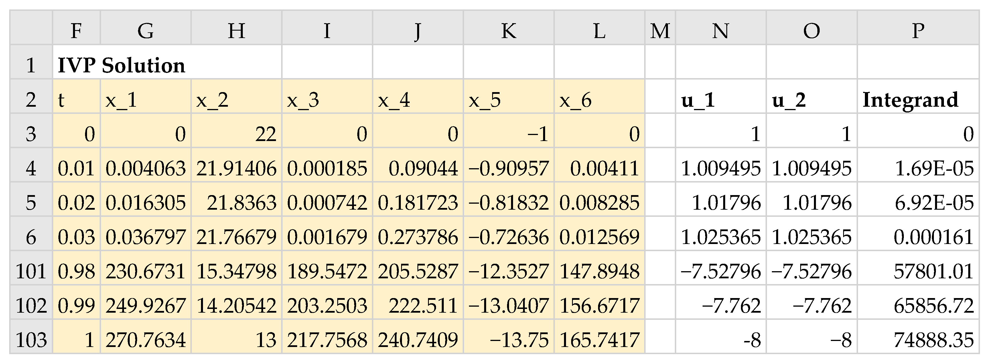
in an allocated array D2:F103. The result is shown partially in Figure 4, and the initial trajectories of x(t), y(t), and u(t) are plotted in Figure 7a.
=IVSOLVE(B11:B12,B2:B4,{0,5})
In order to define the objective formula for the cost functional (6) as described in Task 2 of Section 2, we first generated, based on the obtained initial solution array, two new columns labeled u and Integrand (see Figure 4) for the control function and the integrand expression. The control column, u, was generated with the AutoFill feature of Excel, using the formula H3 shown in Table 1. The integrand column was generated in a similar way using the formula J3 in Table 1. Here, we simply evaluated the expression using the corresponding output solution values for t, x, and y from the IVSOLVE solution.
Next, we employed the discrete data integrator function QUADXY to integrate the generated integrand column versus the solution output times column, as shown by formula M3 of Table 1. The initial value of the objective formula was 246.0854, as shown in Figure 4. To impose the bound constraint (10) on u(t), we defined two aid formulas in M6 and M7 (see Table 1) which computed the maximum and minimum of the generated control column values. We made use of these aid formulas during the configuration of the NLP Solver.
3.1.2. Results and Discussion
We invoked Excel’s Solver from the Data Tab which brings up a dialog as shown in Figure 5. We configured the Solver to minimize the objective formula M3 by varying the control parameters B6:B8 (corresponding to switchT, stage1 and stage2) subject to the constraints
which are needed impose (10). We unchecked the box which reads ‘Make Unconstrained Variables Non-Negative’ to allow the variables to take on negative values as well. In the options for the GRG Nonlinear solver, we switched the derivative scheme from the default Forward to Central, and then ran the Solver, which reports a feasible solution in less than 3 s. By accepting the Solver’s solution, all the values and plots in the spreadsheet were automatically updated to reflect the optimal result. The NLP Solver also generates an optional Answer Report, as shown in Figure 6. The optimal trajectories are plotted in Figure 7b. As shown in the Answer Report, the optimal switching time was found at approximately 1.26 which is within 1% of the 1.25 value reported by Elnagar and Kazemi [17] using a pseudo-spectral Chebyshev approximation of order 15. (In [17], the time domain was transformed to [−1, 1], and the switching time was found at negative 0.5 which maps to 1.25 in the original [0, 5] time domain.)
M6 ≤ 0.8 corresponds to max(u) ≤ 0.8,
M7 ≥ −0.8 corresponds to min(u) ≥ −0.8,
3.2. Unconstrained Nonlinear Optimal Control Problem
The second example represents an unconstrained optimal control problem in the fixed interval , but with highly nonlinear equations. The mathematical problem is stated as follows:
Minimize
subject to
3.2.1. Spreadsheet Model
The spreadsheet model for the IVP (13)–(15) with a parametrized control function using a third-order polynomial is shown in Figure 8. The initial solution to the IVP was obtained by evaluating the formula
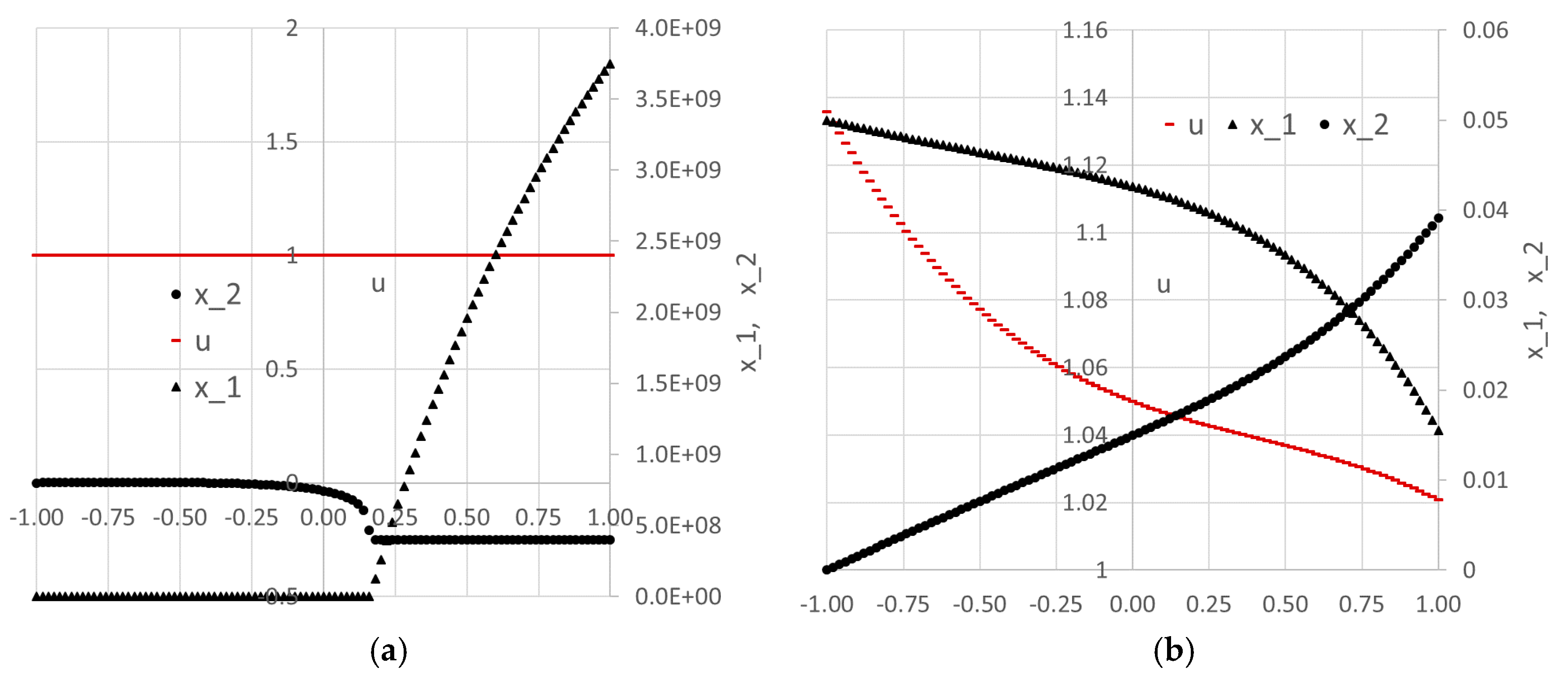
in an allocated array E2:G103, which is shown partially in Figure 9 and plotted in Figure 10a. Clearly, our initial guess for the control coefficients B6:B9 was not good, since the solution exhibits instabilities at larger time values. The control and integrand vectors, needed to construct the objective formula for the cost index (12), were generated based on the obtained initial solution using formulas I3 and K3, listed in Table 2. The objective formula was defined using the data integrator QUADXY as shown in N3 of Table 2, with an initial value of 1.92 × 10¹⁸, as shown in Figure 9.
=IVSOLVE(B12:B13,B2:B4,{−1,1})
3.2.2. Results and Discussion
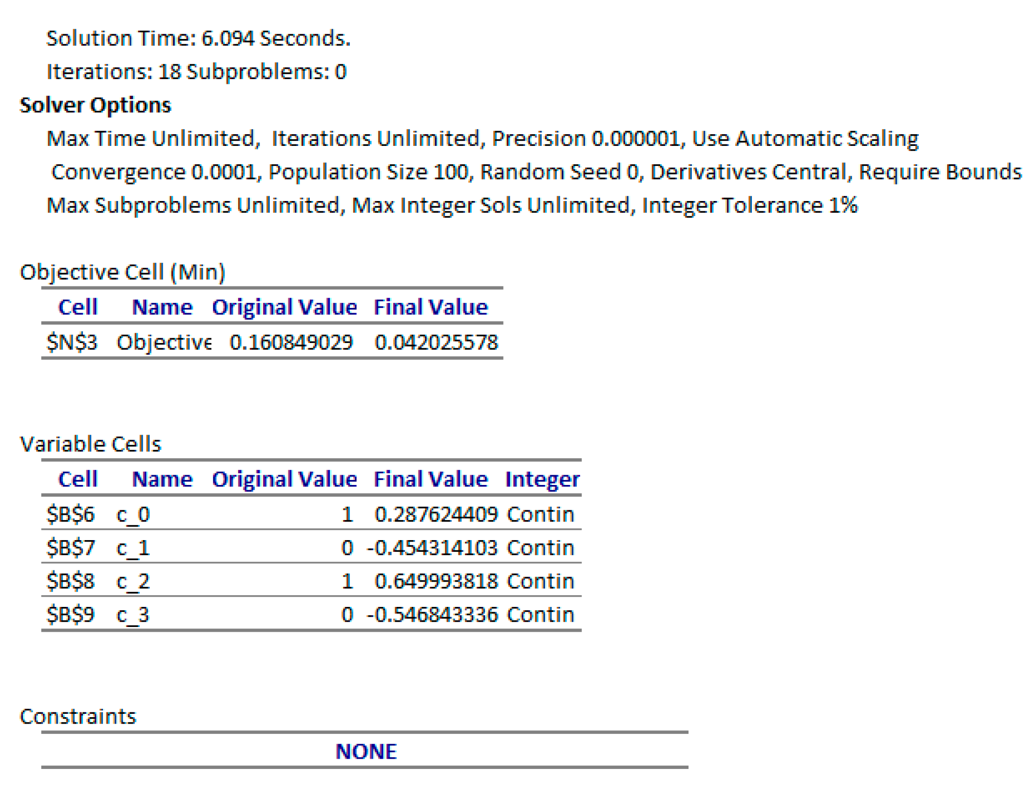
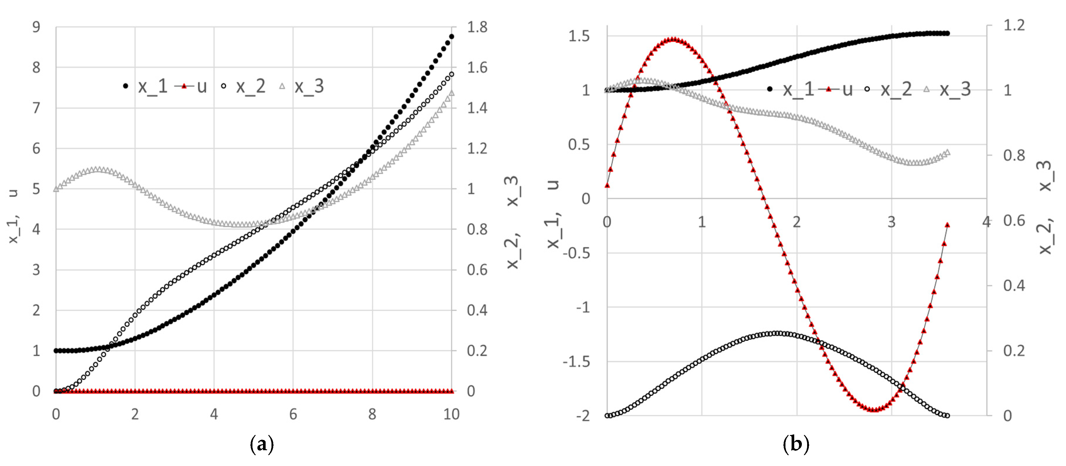
We ran Excel’s Solver to minimize the objective formula N3 by varying the control parameters in B6:B9 with no added constraints. Despite the bad initial values for the control parameters, the Solver reported a feasible solution in about 2 seconds with the Answer Report shown in Figure 11. The optimal trajectories for the system variables are plotted in Figure 10b.
The reported objective in [17] is 0.026621417, which is better than the achieved objective value of 0.08919 found by Excel. To improve the result, we tried a different initial guess for the parameters (c_0, c_1, c_2, c_3) by changing their values in Figure 8 to (1, 0, 1, 0). A second run of the Solver reported the feasible solution shown in Figure 12. The new objective value was reduced by more than 50% to 0.040245. The new solution is plotted in Figure 13 and shows noticeably different trajectories for x_1 and x_2 than those obtained initially in Figure 10. This is expected, given the highly nonlinear and unconstrained problem.
3.3. Minimal Swing Container Transfer Problem
The third example represents the problem of transferring containers, driven by a hoist motor and a trolley drive motor, from a ship to a cargo truck. The goal is to minimize the swing during and at the end of the transfer. The mathematical optimal control problem is described by (17)–(29). The problem is nonlinear with six state variables and two controllers subject to multiple final and bound constraints.
Minimize
subject to
Initial conditions:
Final conditions:
Bounds:
3.3.1. Spreadsheet Model
Following the same procedure as that in the previous examples, we prepared the spreadsheet model for the IVP (18)–(24) using third-order parametrized polynomial control functions and , as shown in Figure 14. Initial values and guesses were assigned to the state variables and unknown parametrization coefficients as shown in the figure. Figure 15 shows a partial listing of the initial solution obtained by evaluating the formula
in array F2:L103, and the generated control columns, u_1, u_2, and the integrand expression column using the corresponding formulas listed in Table 3. The initial system trajectories are plotted in Figure 16.
=IVSOLVE(B17:B22,B2:B8,{0,1})
Next, we defined the objective formula, S3, corresponding to the cost index (17) as shown in Table 3, in which the data integrator QUADXY was used to integrate the generated integrand expression values. The objective formula evaluated to an initial value of 24,229.22793. Table 3 also lists a number of aid formulas which compute the minimum and maximum values for the state variables x_4 and x_5 and the generated control columns. These aid formulas were used to define the bound constraints for the NLP Solver.
3.3.2. Results and Discussion
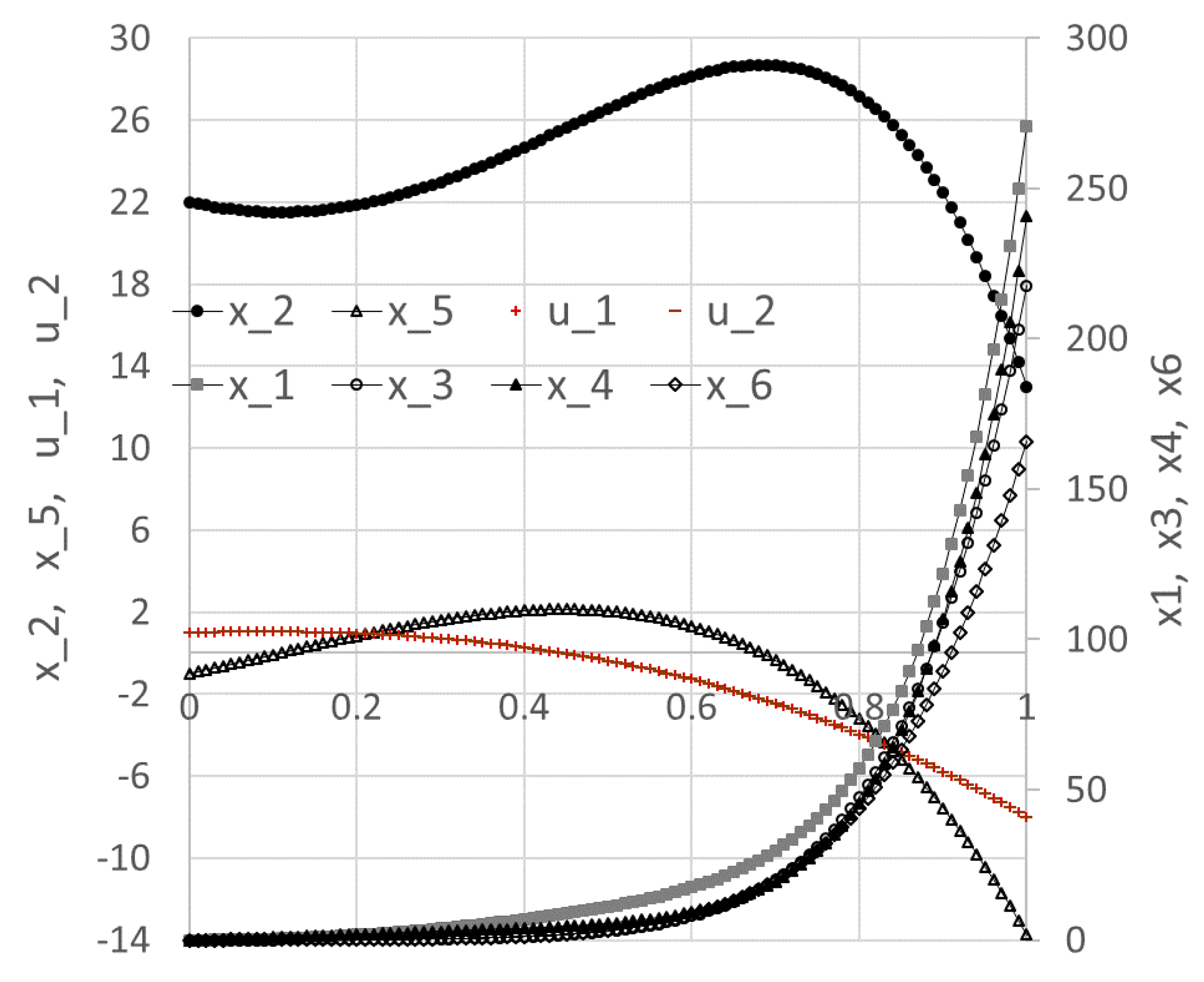
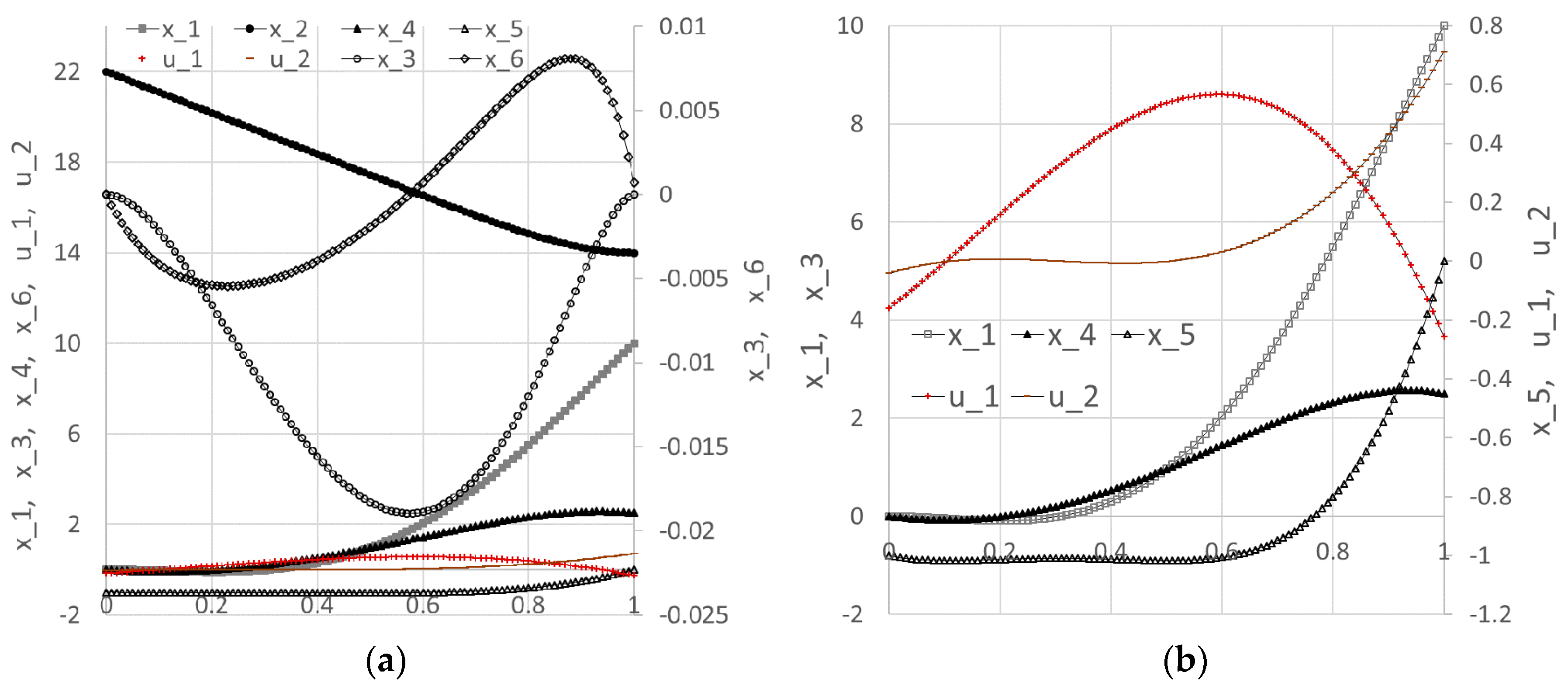
We configured Excel’s Solver to minimize the objective formula S3 by varying the controls’ coefficients B10:B14 and D10:D14 subject to the added constraints listed in Table 4. Here, we made use of the aid formulas listed in Table 3 to define the inequality bound constraints (26)–(29). The end point equality constraints on the state variables (25) were imposed directly onto the corresponding cells at t = 1 (last row) of the IVSOLVE solution array (see Figure 15). The Solver spun for a few seconds, then reported that it did not find a feasible solution when, in fact, it already had, judging by the best-found solution results shown partially in Figure 17 and plotted in Figure 18. The solution indicates that all constraints were satisfied within a reasonable tolerance of 1 × 10⁻⁵, except for x_6(1), which was satisfied within a tolerance of 1 × 10⁻³. This is verified by the feasibility report generated by the Solver, and shown in Figure 19. The report indicates that the Solver had difficulty satisfying end point constraints for x_4 and x_6 at the Solver’s default tolerances, while all other constraints were satisfied.
3.4. Minimum Time Orbit Transfer Problem
The fourth example describes a minimum time orbit transfer problem. The goal is to minimize the transfer time of a constant thrust rocket between the orbits of Earth and Mars, and to determine the optimal thrust angle control. The original free-time mathematical problem is stated as follows:
Minimize
subject to
with initial conditions
and final conditions
In [17], the original problem was transformed into a fixed time domain [−1, 1]. The corresponding value for the transfer time, , was reported at 3.31873 using ninth-degree Chebyshev polynomial approximations. Here, we solve the original free-time problem as stated in (31)–(36).
3.4.1. Spreadsheet Model
Referring to Figure 20, the IVP (32)–(35) was modeled using a third-order parametrized polynomial approximation for , with an initial guess of zero for each of the unknown coefficients. The differential equations in B21:B23 are defined in terms of the system variables in B2:B5, the control u in B19, and the constants , and which are assigned corresponding names in the figure. In this problem, the end time, , is a design variable and is therefore assigned its own variable tF in B13 with an initial guess of 10. Figure 21 shows a partial listing of the initial solution obtained by evaluating the IVSOLVE formula
in array E2:H103, along with the generated control column and the initial objective value. The corresponding formulas are listed in Table 5, and the initial trajectories for the system states and control are plotted in Figure 23a. Note that the third argument to the IVSOLVE formula is the variable time domain which is represented by the range B12:B13.
=IVSOLVE(B21:B23,B2:B5,B12:B13)
3.4.2. Results and Discussion
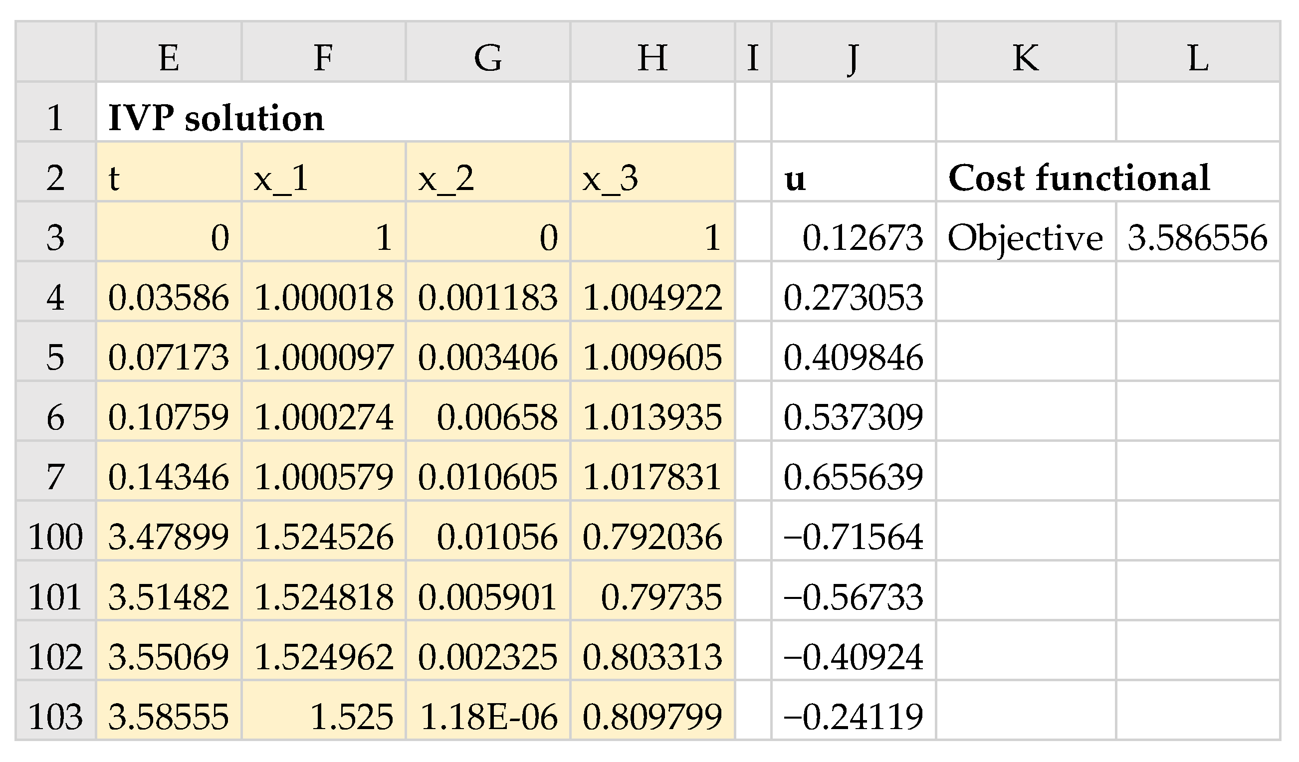
We configured Excel’s Solver to minimize the objective formula L3 by varying the end time tF, B13, and the control coefficients B15:B18, subject to the end point equality constraints on the state variables (36). The constraints were added directly into the Solver’s dialog by referencing the corresponding cells in the last row of the IVSOLVE solution array in Figure 21. The Solver reported, in under 20 s, the feasible solution shown in the Answer Report of Figure 22. The minimum orbit time, , was found to be 3.58656. This compares reasonably well to the value reported in [17] at 3.31873 using ninth-degree Chebyshev polynomial approximations. The optimal trajectories are plotted in Figure 23b. In Figure 24, we show a partial listing of the updated IVSOLVE solution result reflecting the new end time, and the decreased output time increment in comparison to the initial result shown in Figure 21.
4. Practical Tips
Successful nonlinear optimization is often the result of numerical experimentation. In this section, we share a few practical tips for effective use of the presented spreadsheet optimization method.
4.1. Excel’s NLP Solver and Settings
The standard NLP Solver shipped with Excel uses the Generalized Reduced Gradient algorithm [14], which has proved effective for smooth nonlinear problems. The standard Solver also offers a simplex and evolutionary genetic algorithm options that may be suitable for linear or nonsmooth problems. Nonetheless, it is possible to expand the available pool of NLP algorithms, including sequential programming, interior point, and active set methods, by upgrading to a premium version of the NLP Solver [18].
Perhaps the most important factor is the starting guess for the decision parameter vector which may require a nonzero initial value for some problems. The author has found it generally quick to find a good initial guess interactively by trial and error in just a few attempts given the fast response of the Solver. Excel Solver’s dialog offers a few settings, two of which have proved influential in aiding the convergence for some problems. In particular, the ‘Derivatives’ scheme is recommended to be switched to Central from the default Forward, and the ‘Use Automatic Scaling’ option is recommended to be left enabled (default setting).
4.2. Spreadsheet Tips
- Naming spreadsheet variables (e.g., naming B1 as t) makes the formulas easier to read and spot errors. However, it is also recommended to restrict the scope of a named variable to the specific sheet it will be used on, and not the whole workbook. This prevents accidental interdependence between multiple problems on different sheets sharing variables with the same name.
- The shown layouts for the model setup with labels ensures that the Answer Report generated by Excel’s Solver has proper descriptive names for the variables and constraints.
- Excel gives precedence to the unary negation operator which may be confused with the binary minus operator since they both use the same symbol. This can lead to hard-to-find errors in formulas. For example, Excel evaluates the formula ‘=−X1^2’ as ‘=(−X1)^2’. The intention may have been to do ‘−(X1^2)’ instead. A simple fix is to either use parentheses when needed, or to use the intrinsic POWER(X1,2) function instead of the operator ^. Also, when using the IF statement in a formula, it is important to verify that the formula evaluates to a numeric value for all possible conditions. Otherwise, the formula may evaluate to a nonnumeric Boolean condition, leading to a solver error.
- The calculus functions are designed to operate in two modes: a silent mode, where only standard spreadsheet errors are returned like #VALUE!, and a verbose mode, where the function may display an informative error or warning message alert in a popup window. It is recommended to work in the verbose mode when setting up the problem, but switch to the silent mode before running the NLP Solver. Switching between the two modes is triggered by evaluating the formula ‘=VERBOSE(TRUE)’ or ‘=VERBOSE(FALSE)’ in any cell in the workbook. For some problems, the Solver may wander into illegal input space before it recovers and adjusts its search. The silent mode blocks any occasional error alerts from the calculus functions.
4.3. Generalization to a Special Class of Control Problems
By restricting the space of admissible control functions to, for example, variable-order polynomials up to a fixed degree, it may not be always possible to find a solution to a certain class of control problems for which the optimal control, in fact, lies outside the admissible space. It is difficult to know a priori when an algorithm may or may not work, but this may arise in problems with a particularly long time horizon. When all fails, it may well be that the only alternative is to use an indirect method and maximize the Hamiltonian for a number of points, then use interpolation to construct the complete control function(s). Nonetheless, we propose below a general idea that we have not tested but which fits within our presented direct method, and may offer a potential solution in certain cases.
The idea, effectively, is to enlarge the admissible space by stitching together different parametrized control functions defined over nonoverlapping subintervals of the time horizon. Both the interior end points of the subintervals (stitching points), and the control functions’ parameters are unknown design variables for the NLP Solver. The stitching is enforced by imposing additional constraints for the NLP Solver that demand continuity of the control functions at the stitching points. A continuity condition is easily derived algebraically by matching two parametrized functions’ values at a stitching point. Excel NLP Solver poses no restriction on the number of design variables, although performance and convergence will be impacted as the problem dimension grows.
5. Conclusions
We have demonstrated a practical technique which adapts the control parametrization direct method for optimal control problems to the spreadsheet. The technique combines Excel’s NLP Solver command with two calculus worksheet functions, an initial value problem solver, and a discrete data integrator in a simple systematic procedure. The employed calculus functions are utilized from an Excel calculus Add-in library [19]. The technique has proved very effective on several highly nonlinear, multivariable, constrained control problems, and produced results consistent with reported answers obtained with highly accurate pseudo-spectral approximation and NLPQL optimization software package using a full parametrization direct method. Excel’s Solver’s computing time has been in the order of seconds to a minute on a laptop with an Intel 4-Core i7 CPU, which makes the technique highly interactive for experimenting with different initial guesses and variations. As demonstrated by the examples, using the devised method requires no more than defining a few formulas with basic knowledge of the spreadsheet and requires no programming skills, offering a simpler solution approach to optimal control problems.
A slightly modified version of the technique can also be applied for parameter estimation of initial value problems where the parameters may include initial conditions or coefficients. In future work, it may also be worth investigating a dual technique based on indirect methods for optimal control problems. The indirect method requires the modeler to recast the problem in a different form by applying Pontryagin’s maximum principle. However, the ensuing boundary value problem could be solved with the aid of a boundary value problem solver function, BVSOLVE, also included in the Excel calculus Add-in [19].
Supplementary Materials
An Excel workbook containing all the solved examples presented in this article is available at https://www.mdpi.com/2297-8747/23/1/6/s1, (file Location to be determined.)
Acknowledgments
No funding has been received in support of this research work.
Conflicts of Interest
The author of the manuscript is the founder of ExcelWorks LLC of Massachusetts, USA supplying the Excel calculus Add-in, ExceLab, utilized in this research work.
Appendix A
Appendix A.1. Initial Value Problem Solver Spreadsheet Function
The spreadsheet function
is utilized from the calculus Add-in [19] to solve an initial value ordinary differential algebraic equation system in the interval :
, and M is an optional mass matrix. If M is singular, the system is differential algebraic. IVSOLVE implements several adaptive integration schemes [12,20], suitable for stiff and smooth problems. By default, it uses the RADUA5 algorithm [12]. Algorithm selection and control parameters, as well as the system analytic Jacobian can be supplied via optional arguments [19]. At minimum, IVSOLVE requires three arguments:
=IVSOLVE(equations, variables, time_interval, mass_matrix, options)
- Reference to the right-hand side formulas corresponding to the vector-valued function . Any algebraic equations should be ordered last.
- Reference to the system variables corresponding to t and in the specific order ().
- The integration time interval end points.
IVSOLVE is run as a standard array formula in an allocated array of cells. It evaluates to an ordered tabular result where the time values are listed in the first column and the corresponding state variables’ values are listed in adjacent columns. By default, IVSOLVE reports the output at uniform intervals according to the allocated number of rows for the output array. Custom output formats can be achieved via the optional parameters, including specifying custom divisions or output points [19]. We demonstrate IVSOLVE for the following DAE example:
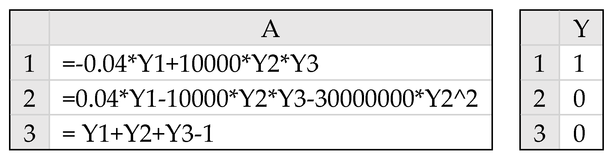
The system RHS formulas are defined in cells A1:A3 using cell T1 for the time variable and Y1, Y2, Y3 for the state variables with the specified initial conditions shown in Figure A1.
Figure A1.
Spreadsheet input model for equation system A2.
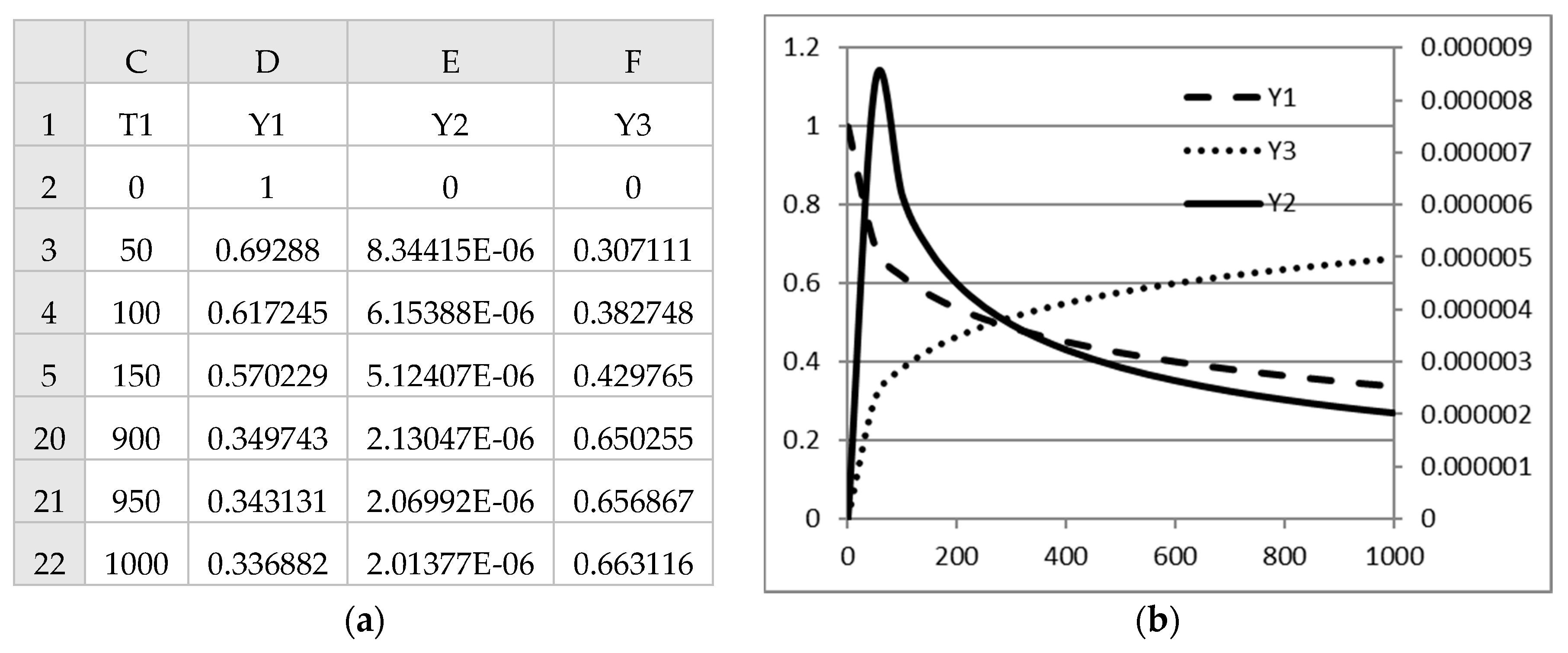
To solve the system, we evaluate in the array C1:F22 the formula
which computes and displays the solution shown in Figure A2. Note that the fourth argument, 1, instructs the solver that the last equation in A1:A3 is an algebraic equation.
=IVSOLVE (A1:A3,(T1,Y1:Y3),{0,1000},1)
Figure A2.
(a) Partial listing of the computed solution by formula A3; (b) Plots of the trajectories.
Figure A2.
(a) Partial listing of the computed solution by formula A3; (b) Plots of the trajectories.
Appendix A.2. Discrete Data Integrator Spreadsheet Function
The spreadsheet function
is utilized from the calculus Add-in [19] to integrate a set of discrete (x, y(x)) data points. The integration limits are determined from the endpoints of the x vector. QUADXY performs the integration with the aid of cubic (default) or linear splines [13]. The third optional argument allows the specification of boundary conditions for the data, including starting and end slopes. Options are specified by (key, value) pairs as detailed in [19].
=QUADXY(x, y, options)
References
- La Torre, D.; Kunze, H.; Ruiz-Galan, M.; Malik, T.; Marsiglio, S. Optimal Control: Theory and Application to Science, Engineering, and Social Sciences. Abstr. Appl. Anal. 2015, 2015, 890527. [Google Scholar] [CrossRef]
- Geering, H.P. Optimal Control with Engineering Applications; Springer: Berlin/Heidelberg, Germany, 2007. [Google Scholar]
- Aniţa, S.; Arnăutu, V.; Capasso, V. An Introduction to Optimal Control Problems in Life Sciences and Economics: From Mathematical Models to Numerical Simulation with MATLAB; Birkhäuser: Basel, Switzerland, 2011. [Google Scholar]
- Böhme, T.J.; Frank, B. Indirect Methods for Optimal Control. In Hybrid Systems, Optimal Control and Hybrid Vehicles. Advances in Industrial Control; Springer: Cham, Switzerland, 2017. [Google Scholar]
- Böhme, T.J.; Frank, B. Direct Methods for Optimal Control. In Hybrid Systems, Optimal Control and Hybrid Vehicles. Advances in Industrial Control; Springer: Cham, Switzerland, 2017. [Google Scholar]
- Banga, J.R.; Balsa-Canto, E.; Moles, C.G.; Alonso, A.A. Dynamic optimization of bioprocesses: Efficient and robust numerical strategies. J. Biotechnol. 2003, 117, 407–419. [Google Scholar] [CrossRef] [PubMed]
- Rodrigues, H.S.; Monteiro, M.T.T.; Torres, D.F.M. Optimal Control and Numerical Software: An Overview. This is a preprint of a paper whose final and definite form will appear in the book. In Systems Theory: Perspectives, Applications and Developments; Miranda, F., Ed.; Nova Science Publishers: Hauppauge, NY, USA, 2014; Available online: https://arxiv.org/abs/1401.7279 (accessed on 23 January 2018).
- Ghaddar, C. Method, Apparatus, and Computer Program Product for Optimizing Parameterized Models Using Functional Paradigm of Spreadsheet Software. U.S. Patent 9,286,286, 15 March 2016. [Google Scholar]
- Ghaddar, C. Method, Apparatus, and Computer Program Product for Solving Equation System Models Using Spreadsheet Software. U.S. Patent 15,003,848, 2018. in Press. [Google Scholar]
- Ghaddar, C. Unconventional Calculus Spreadsheet Functions. World Academy of Science, Engineering and Technology, International Science Index 112. Int. J. Math. Comput. Phys. Electr. Comput. Eng. 2016, 10, 194–200. Available online: http://waset.org/publications/10004374 (accessed on 23 January 2018).
- Ghaddar, C. Unlocking the Spreadsheet Utility for Calculus: A Pure Worksheet Solver for Differential Equations. Spreadsheets Educ. 2016, 9, 5. Available online: http://epublications.bond.edu.au/ejsie/vol9/iss1/5 (accessed on 23 January 2018).
- Hairer, E.; Wanner, G. Solving Ordinary Differential Equations II: Stiff and Differential-Algebraic Problems; Springer Series in Computational Mathematics; Springer: Berlin/Heidelberg, Germany, 1996. [Google Scholar]
- De Boor, C. A Practical Guide to Splines (Applied Mathematical Sciences); Springer: Berlin/Heidelberg, Germany, 2001. [Google Scholar]
- Lasdon, L.S.; Waren, A.D.; Jain, A.; Ratner, M. Design and Testing of a Generalized Reduced Gradient Code for Nonlinear Programming. ACM Trans. Math. Softw. 1978, 4, 34–50. [Google Scholar] [CrossRef]
- Weber, E.J. Optimal Control Theory for Undergraduates Using the Microsoft Excel Solver Tool. Comput. High. Educ. Econ. Rev. 2007, 19, 4–15. [Google Scholar]
- Nævdal, E. Solving Continuous Time Optimal Control Problems with a Spreadsheet. J. Econ. Educ. 2003, 34, 99–122. [Google Scholar] [CrossRef]
- Elnagar, G.; Kazemi, M.A. Pseudospectral Chebyshev Optimal Control of Constrained Nonlinear Dynamical Systems. Comput. Optim. Appl. 1998, 11, 195–217. [Google Scholar] [CrossRef]
- FrontlineSolvers. Available online: https://www.solver.com/ (accessed on 23 January 2018).
- ExcelWorks LLC; MA, USA. ExceLab Calculus Add-in for Excel and Reference Manual. Available online: https://excel-works.com (accessed on 23 January 2018).
- Hindmarsh, A.C. ODEPACK, A Systematized Collection of ODE Solvers. In Scientific Computing; Stepleman, R.S., Carver, M., Peskin, R., Ames, W.F., Vichnevetsky, R., Eds.; North-Holland Publishing: Amsterdam, The Netherlands, 1983; pp. 55–64. [Google Scholar]
Figure 1.
Flowchart for the design of a mathematically pure spreadsheet solver function which accepts formulas as input arguments. Enabling technology is described in [8,9].

Figure 2.
Illustration of the ordered steps for defining an analogous objective formula to the cost index functional (1). The illustration assumes a problem with two state variables and one control.
Figure 2.
Illustration of the ordered steps for defining an analogous objective formula to the cost index functional (1). The illustration assumes a problem with two state variables and one control.

Figure 3.
Spreadsheet model for IVP (7)–(9) with parametrized control function. The colored ranges are input parameters for the IVSOLVE Formula (11).
Figure 3.
Spreadsheet model for IVP (7)–(9) with parametrized control function. The colored ranges are input parameters for the IVSOLVE Formula (11).

Figure 4.
Partial listing of computed results by Formula (11). Also shown are generated control and integrand columns, and initial objective formula value. The associated formulas are listed in Table 1.
Figure 4.
Partial listing of computed results by Formula (11). Also shown are generated control and integrand columns, and initial objective formula value. The associated formulas are listed in Table 1.

Figure 5.
Excel’s Solver dialog configured for optimal control problem (6)–(10).
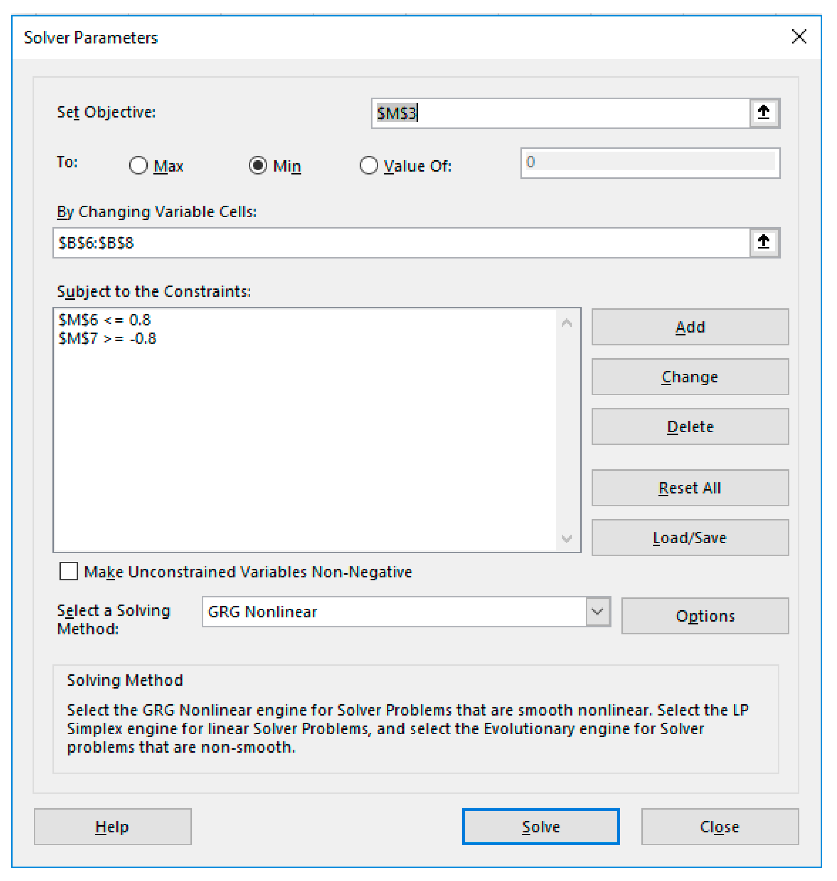
Figure 6.
Answer Report generated by Excel’s Solver for optimal control problem (6)–(10).
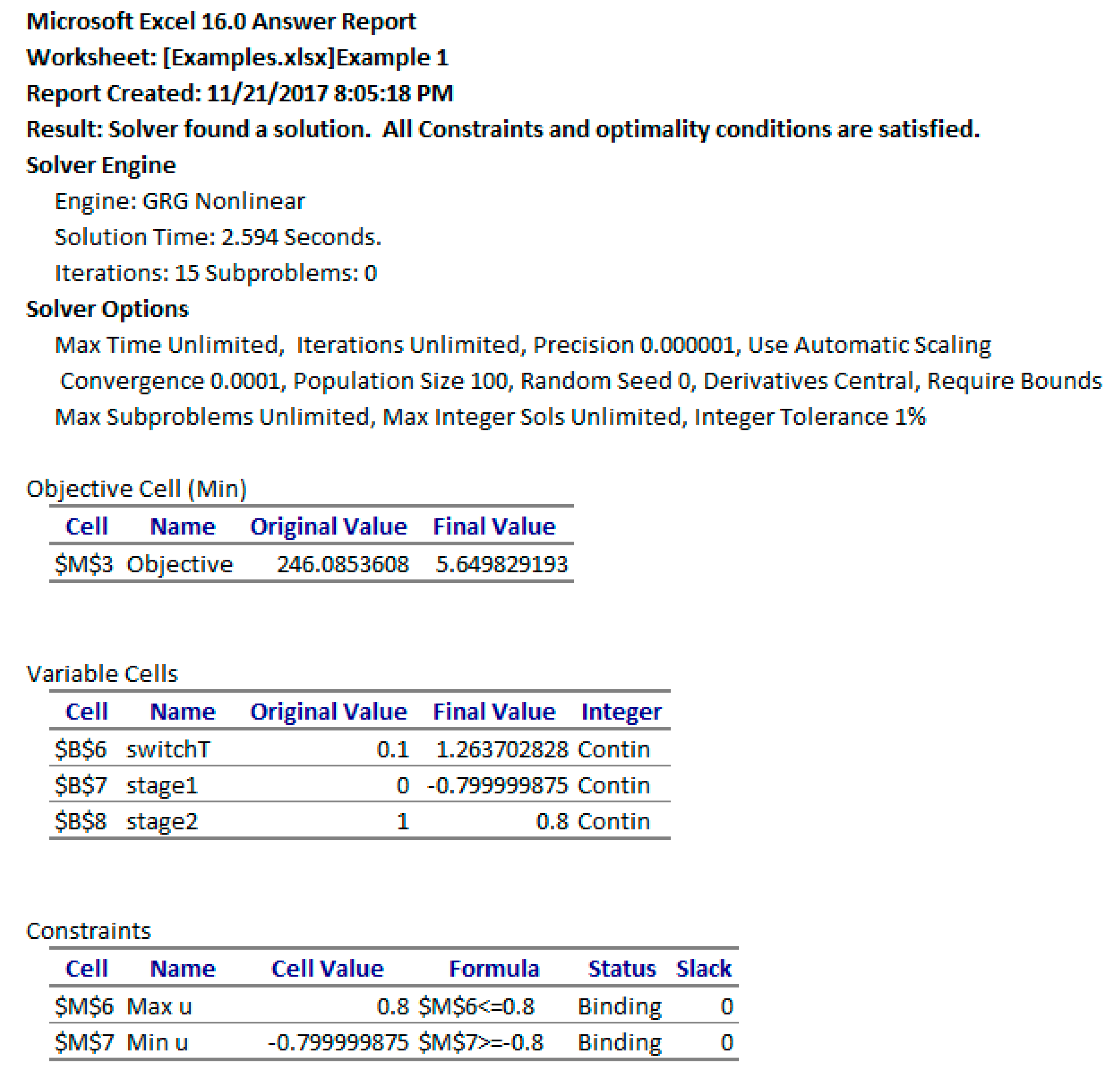
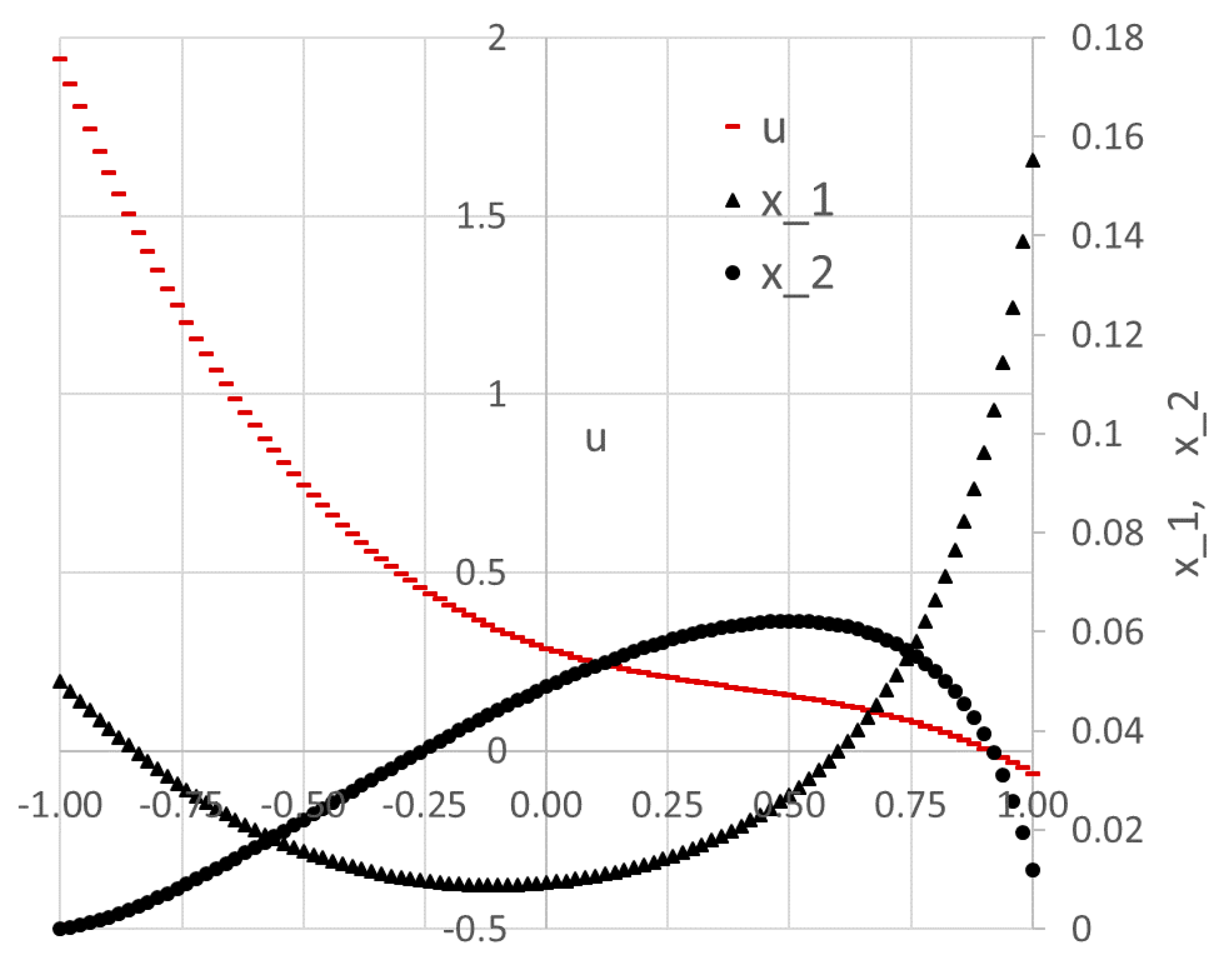
Figure 7.
(a) Initial trajectories for optimal control problem (6)–(10) based on the default values shown in Figure 3; (b) Optimal trajectories found by Excel’s nonlinear programming (NLP) Solver.
Figure 7.
(a) Initial trajectories for optimal control problem (6)–(10) based on the default values shown in Figure 3; (b) Optimal trajectories found by Excel’s nonlinear programming (NLP) Solver.
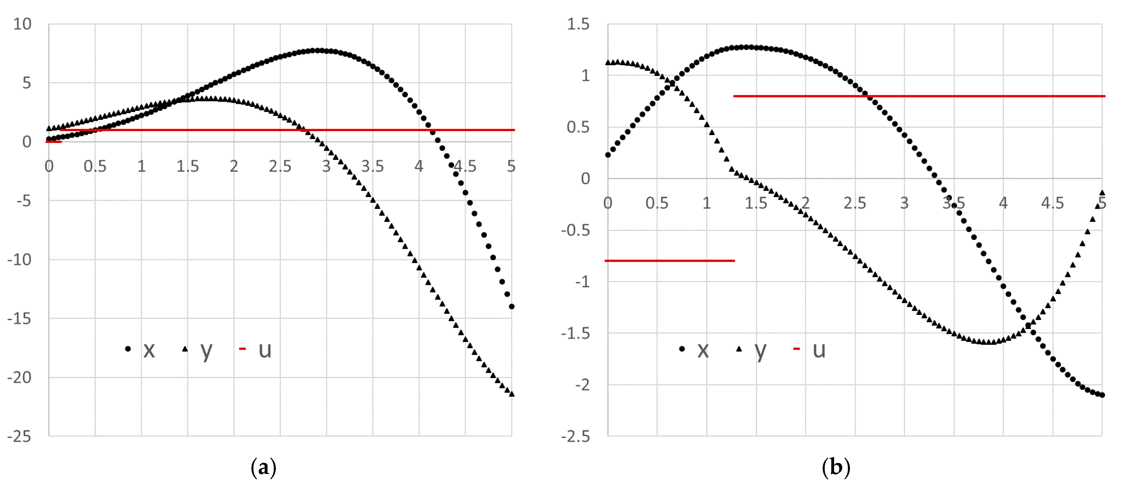
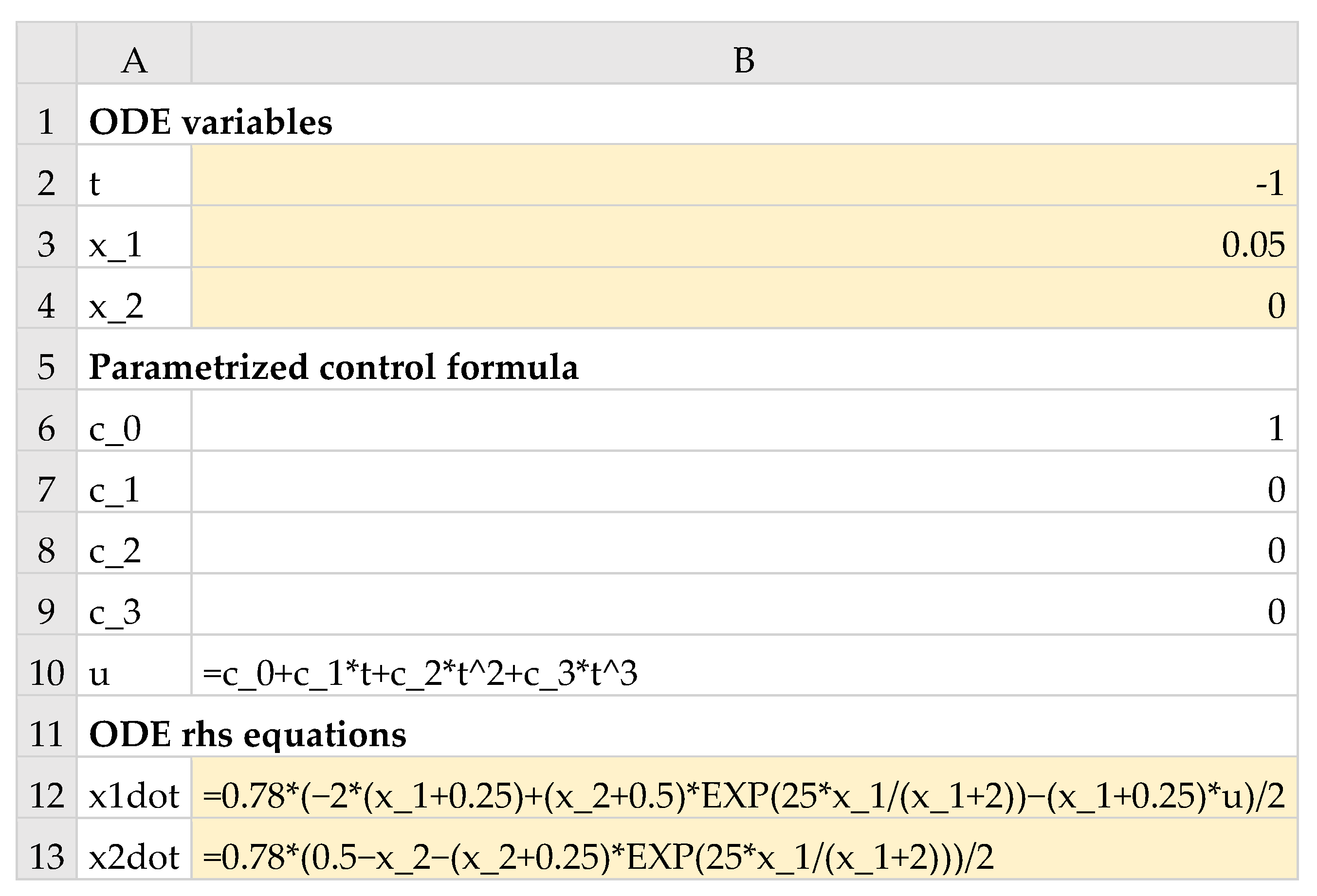
Figure 8.
Spreadsheet model for the IVP (13)–(15) with parametrized control function. The colored ranges are input parameters for IVSOLVE Formula (16).
Figure 8.
Spreadsheet model for the IVP (13)–(15) with parametrized control function. The colored ranges are input parameters for IVSOLVE Formula (16).

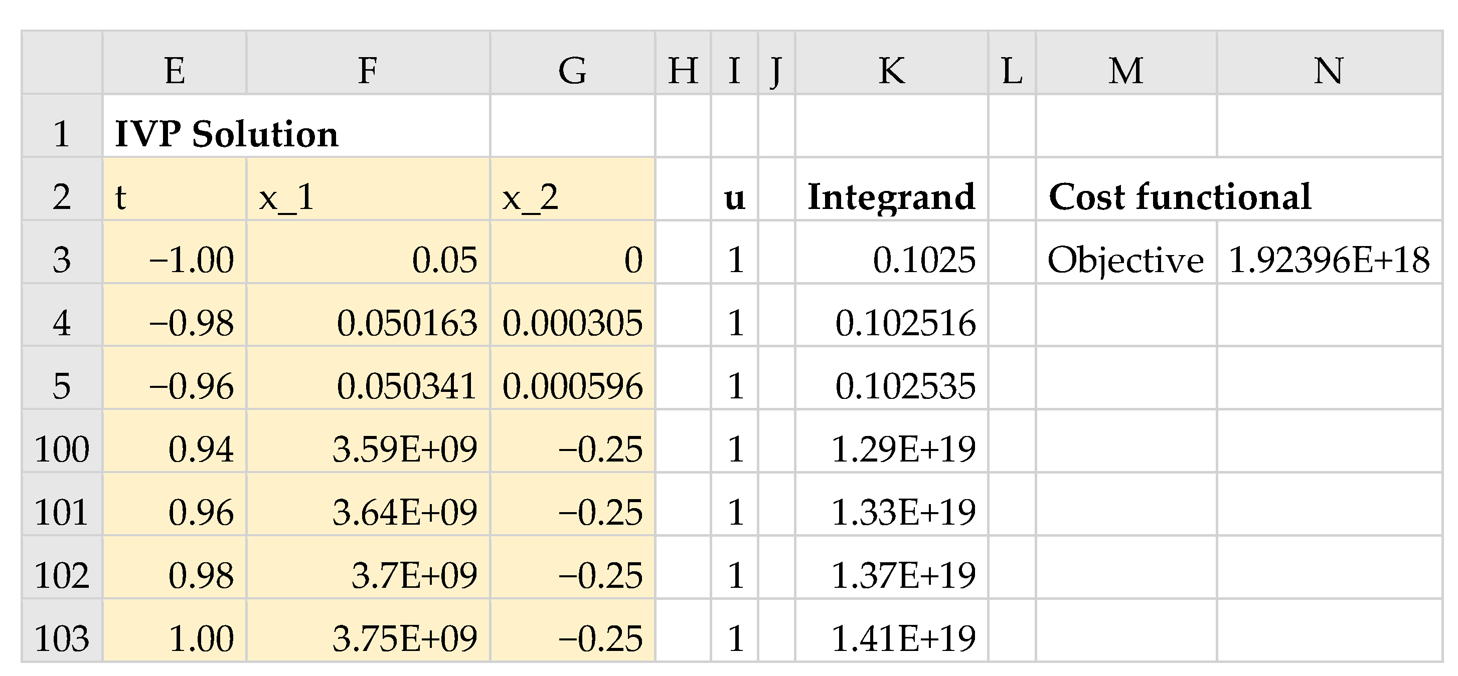
Figure 9.
Partial listing of computed results by Formula (16). Also shown are generated control and integrand columns, and the initial objective formula value. The associated formulas are listed in Table 2.
Figure 9.
Partial listing of computed results by Formula (16). Also shown are generated control and integrand columns, and the initial objective formula value. The associated formulas are listed in Table 2.

Figure 10.
(a) Initial trajectories for optimal control problem (12)–(15) based on the default values shown in Figure 8; (b) Optimal trajectories found by Excel’s NLP Solver.
Figure 10.
(a) Initial trajectories for optimal control problem (12)–(15) based on the default values shown in Figure 8; (b) Optimal trajectories found by Excel’s NLP Solver.

Figure 11.
Answer Report generated by Excel’s Solver for optimal control problem (12)–(15) based on the initial guess values in Figure 8.
Figure 11.
Answer Report generated by Excel’s Solver for optimal control problem (12)–(15) based on the initial guess values in Figure 8.
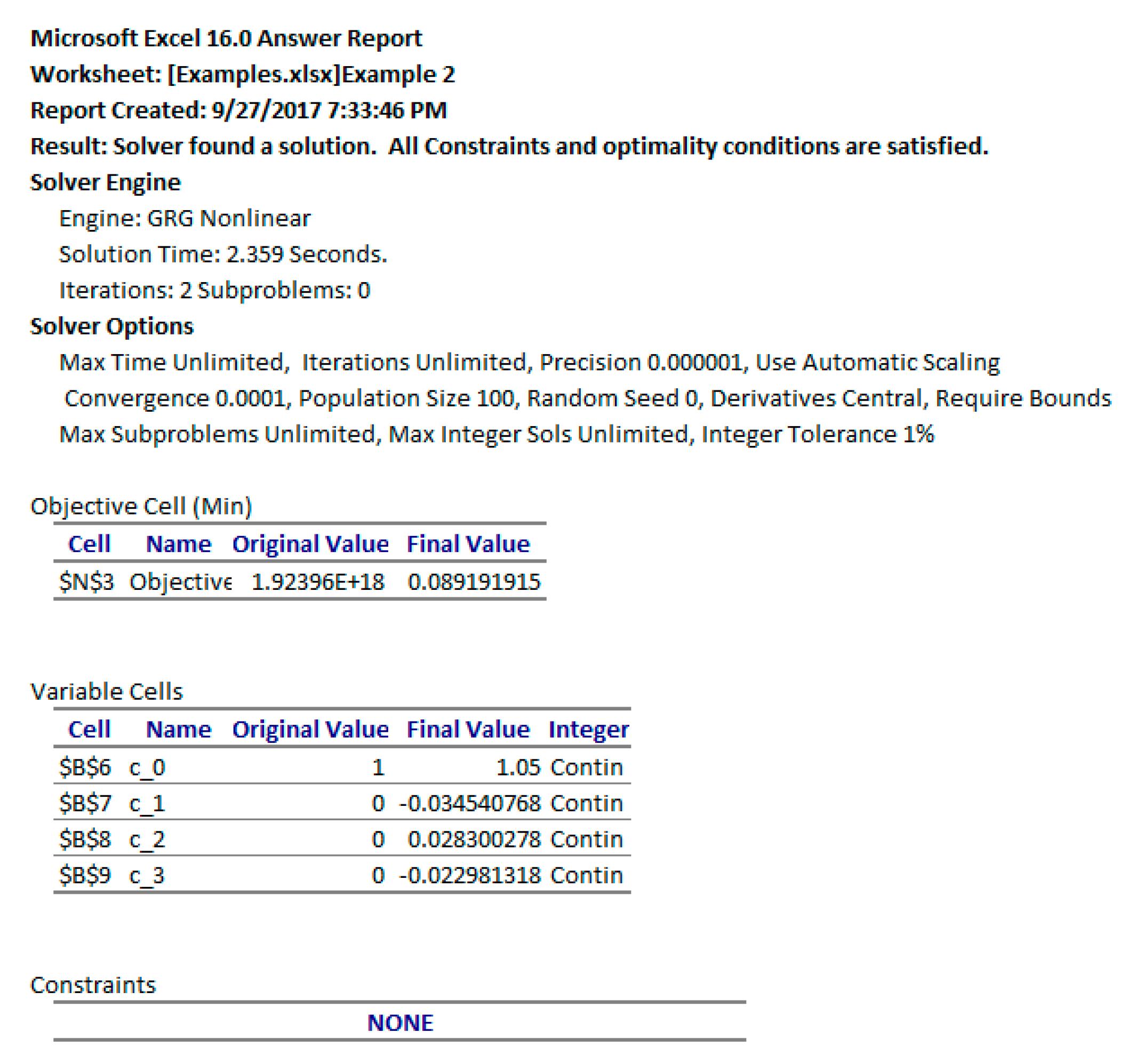
Figure 12.
Answer Report for optimal control problem (12)–(15) using a different initial guess and yielding improved minimum.
Figure 12.
Answer Report for optimal control problem (12)–(15) using a different initial guess and yielding improved minimum.

Figure 13.
Optimal trajectories for optimal control problem (12)–(15) found by Excel’s Solver starting from a different initial guess, leading to a lower objective value.
Figure 13.
Optimal trajectories for optimal control problem (12)–(15) found by Excel’s Solver starting from a different initial guess, leading to a lower objective value.

Figure 14.
Spreadsheet model for the IVP (18)–(24) with parametrized control functions. The colored ranges are input parameters for IVSOLVE Formula (30).
Figure 14.
Spreadsheet model for the IVP (18)–(24) with parametrized control functions. The colored ranges are input parameters for IVSOLVE Formula (30).

Figure 15.
Partial listing of computed result by Formula (30). Also shown are generated control and integrand columns. The associated formulas are listed in Table 3.
Figure 15.
Partial listing of computed result by Formula (30). Also shown are generated control and integrand columns. The associated formulas are listed in Table 3.

Figure 16.
Initial trajectories for optimal control problem (17)–(29) based on default values shown in Figure 14.
Figure 16.
Initial trajectories for optimal control problem (17)–(29) based on default values shown in Figure 14.

Figure 17.
Best-found solution obtained by Excel’s Solver for optimal control problem (17)–(29).
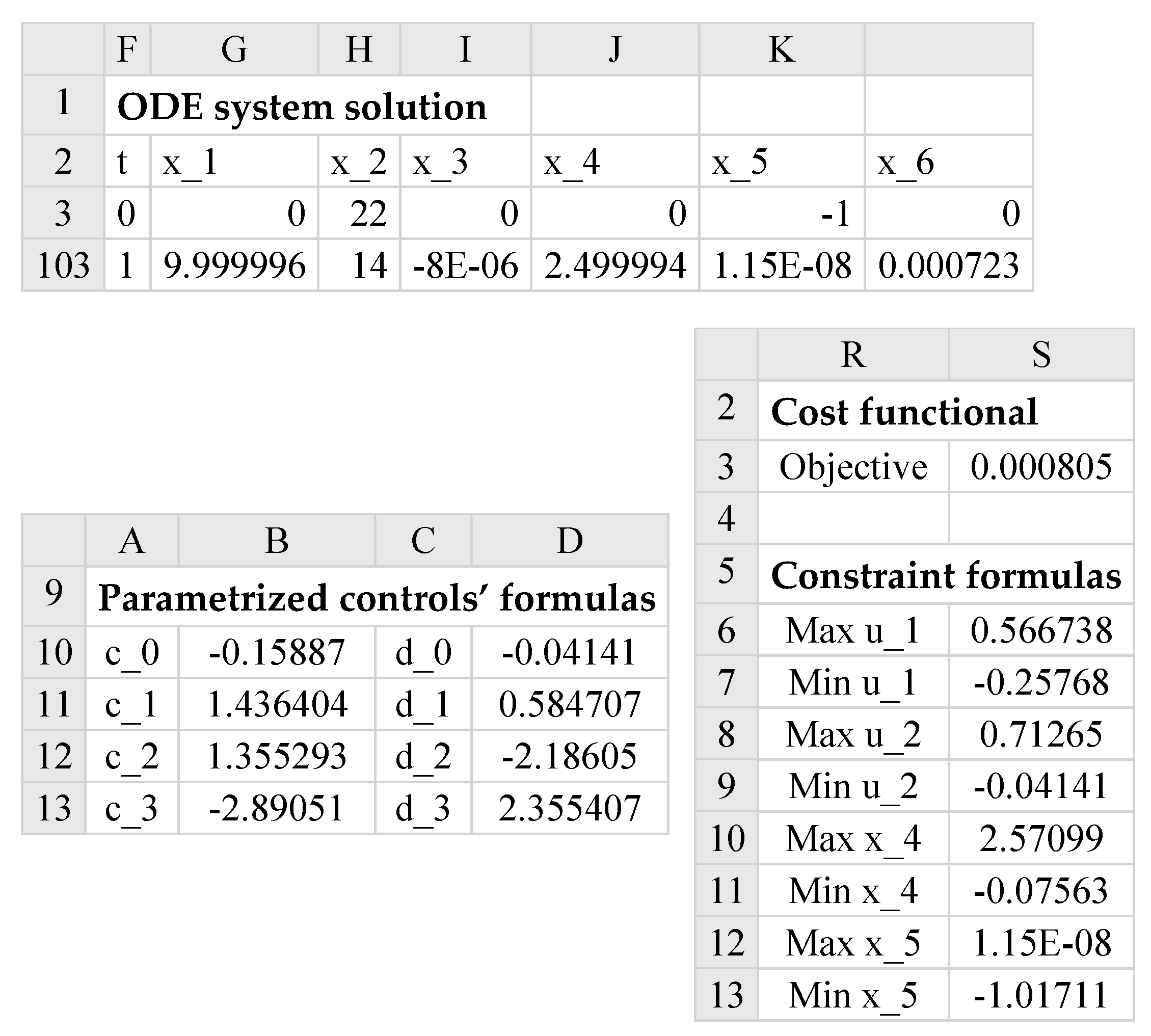
Figure 18.
(a) Optimal trajectories for all variables of optimal control problem (17)–(29); (b) Selected optimal trajectories.
Figure 18.
(a) Optimal trajectories for all variables of optimal control problem (17)–(29); (b) Selected optimal trajectories.

Figure 19.
Feasibility Report generated by Excel’s Solver for optimal control problem (17)–(29).
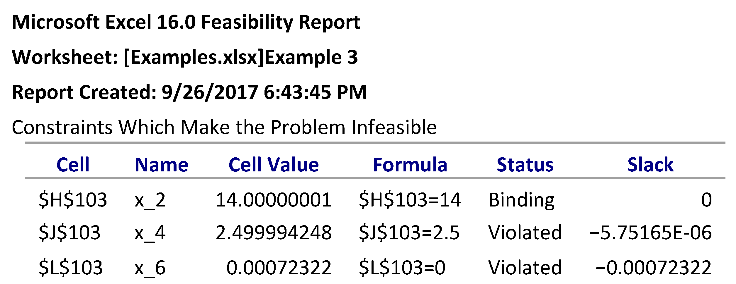
Figure 20.
Spreadsheet model for the IVP (32)–(35) with parametrized control function. The colored ranges are input parameters for IVSOLVE Formula (37).
Figure 20.
Spreadsheet model for the IVP (32)–(35) with parametrized control function. The colored ranges are input parameters for IVSOLVE Formula (37).
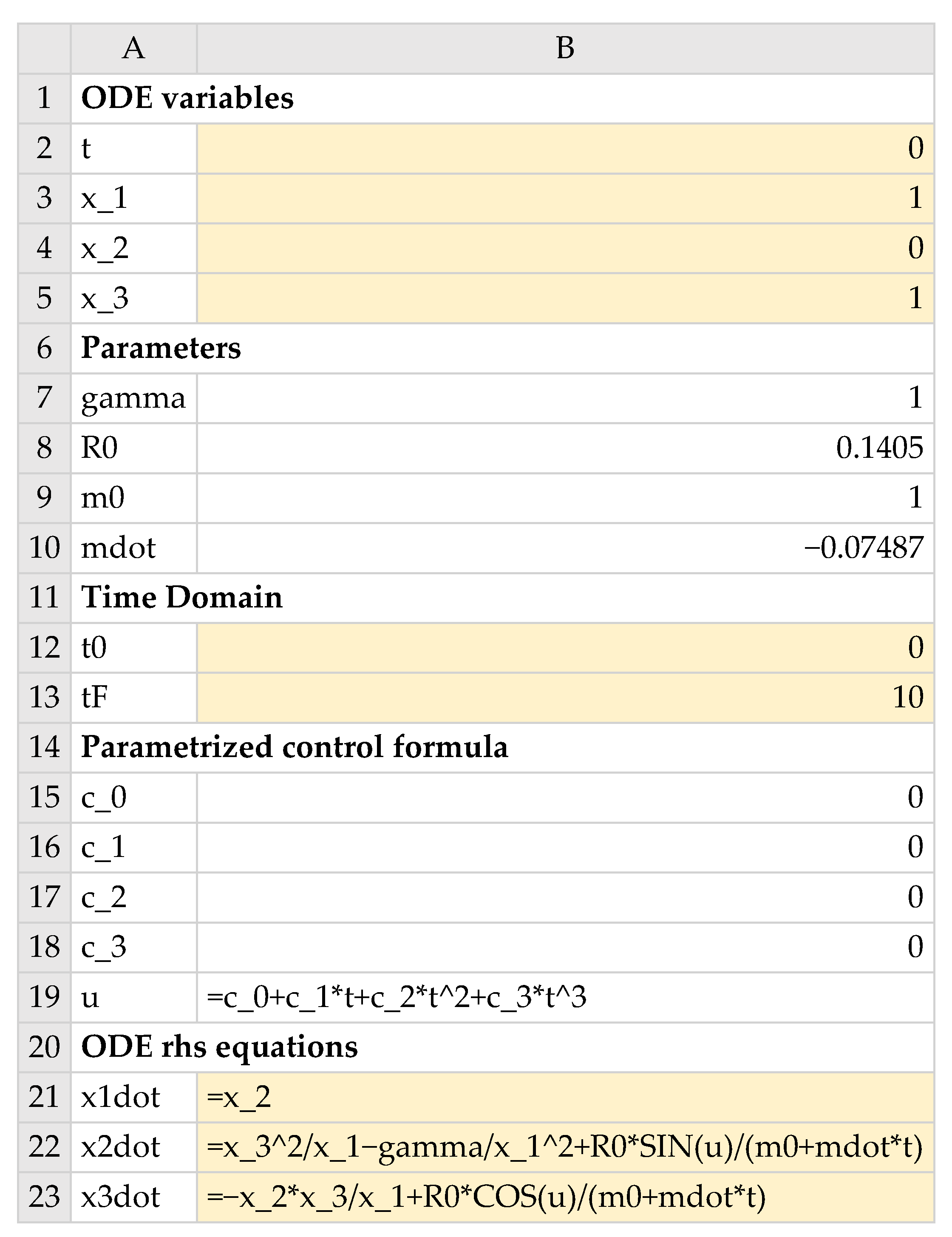
Figure 21.
Partial listing of computed result by Formula (37). Also shown are generated control column and the initial objective formula value. The associated formulas are listed in Table 5.
Figure 21.
Partial listing of computed result by Formula (37). Also shown are generated control column and the initial objective formula value. The associated formulas are listed in Table 5.
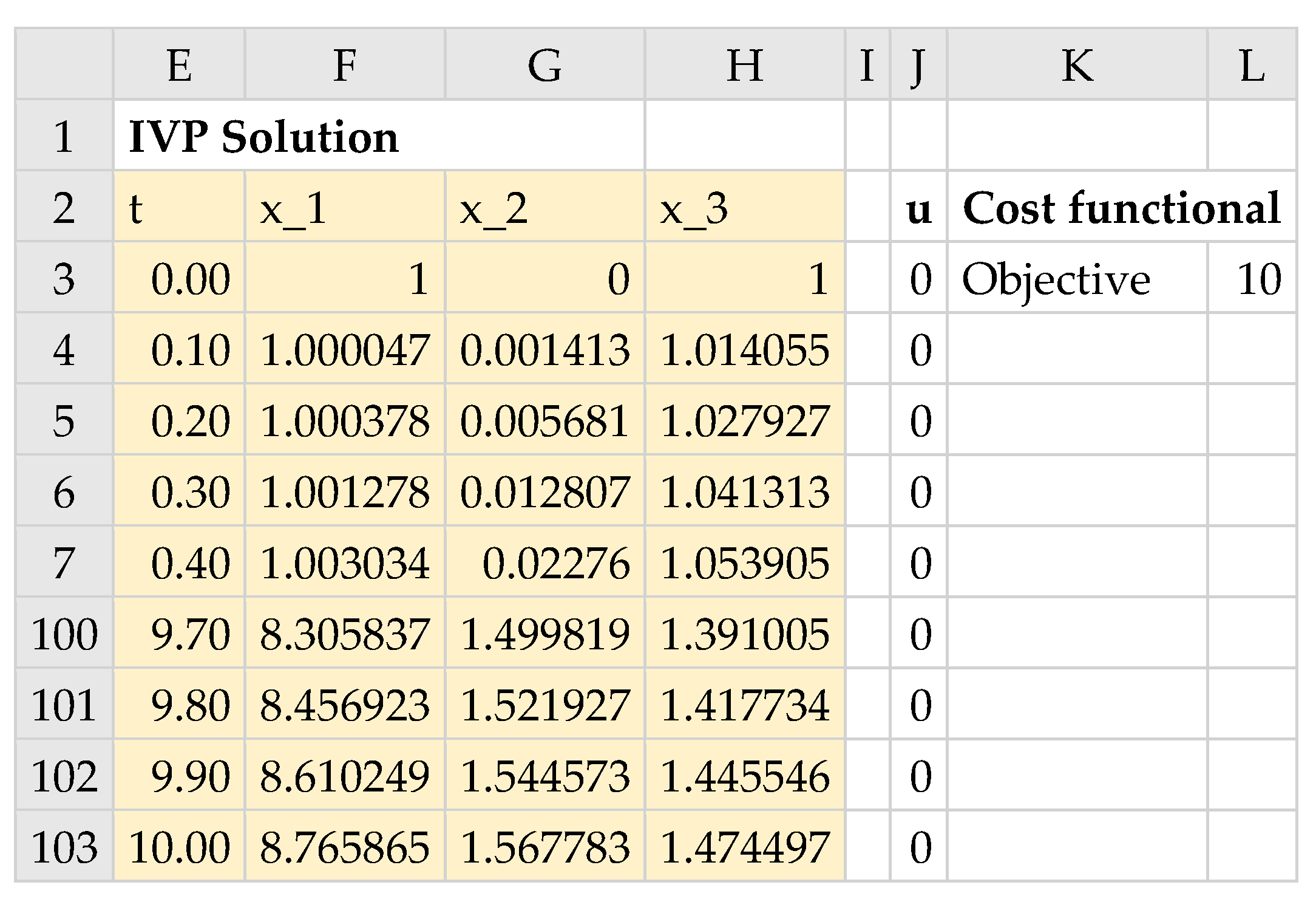
Figure 22.
Answer Report generated by Excel’s Solver for optimal control problem (31)–(36).
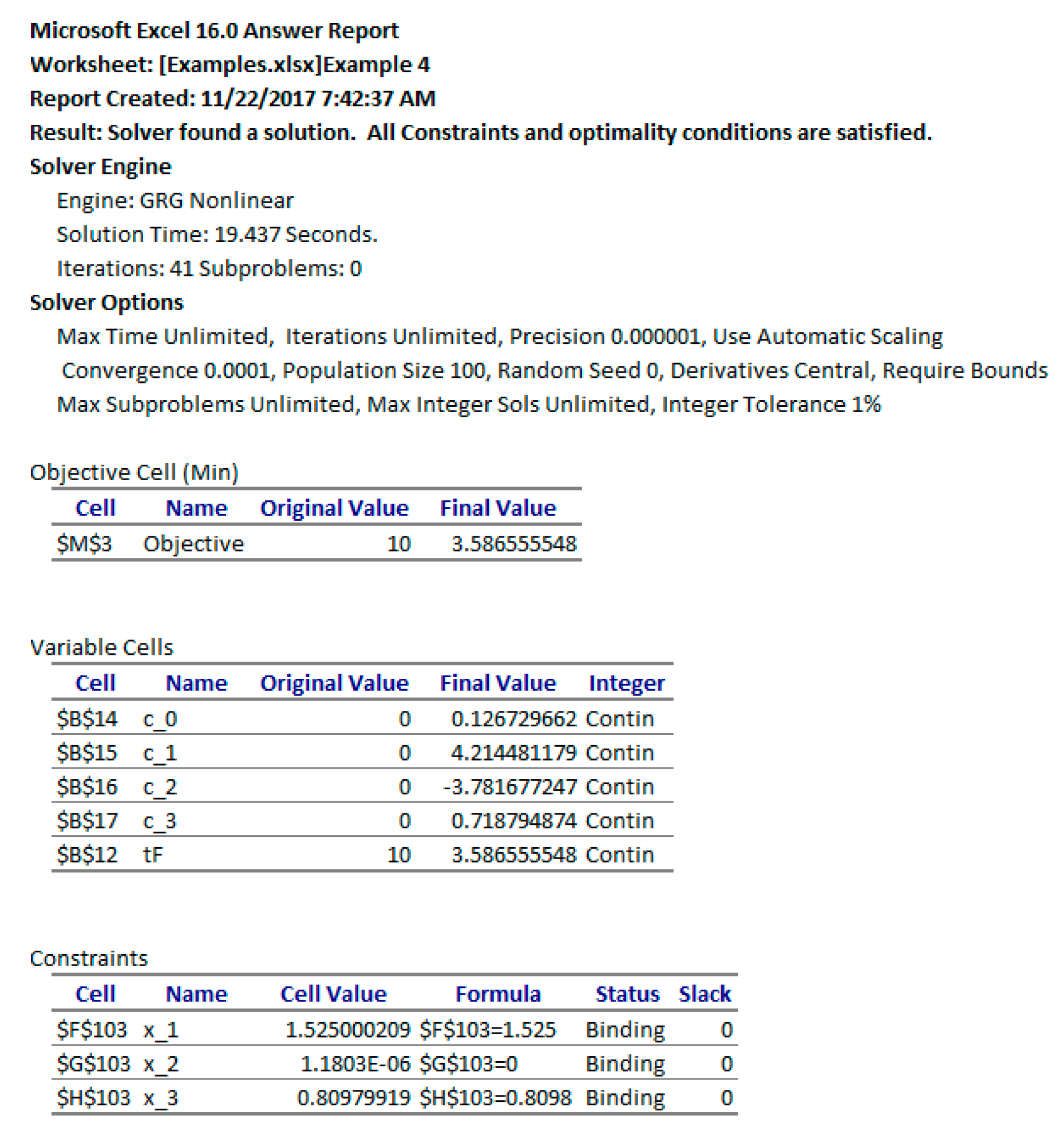
Figure 23.
(a) Initial trajectories for optimal control problem (31)–(36) based on default values shown in Figure 20; (b) Optimal trajectories found by Excel’s NLP Solver.
Figure 23.
(a) Initial trajectories for optimal control problem (31)–(36) based on default values shown in Figure 20; (b) Optimal trajectories found by Excel’s NLP Solver.

Figure 24.
Partial listing of the updated initial result of Figure 21 which reflects the optimal final time and adjusted output time values in Column E.
Figure 24.
Partial listing of the updated initial result of Figure 21 which reflects the optimal final time and adjusted output time values in Column E.

Table 1.
Formula definitions used for solving optimal control problem (6)–(10).
| Purpose | Cell | Formula |
|---|---|---|
| Initial value problem solution | D2:F103 | =IVSOLVE(B11:B12,B2:B4,{0,5}) |
| AutoFill formula for control values | H3 | =IF(D3<=switchT,stage1,stage2) |
| AutoFill formula for integrand values | J3 | =E3^2+F3^2 |
| Objective formula | M3 | =0.5*QUADXY(D3:D103,J3:J103) |
| Maximum value of control column | M6 | =MAXA(H3:H103) |
| Minimum value of control column | M7 | =MINA(H3:H103) |
Table 2.
Formula definitions used for solving optimal control problem (12)–(15).
| Purpose | Cell | Formula |
|---|---|---|
| Initial value problem solution | E2:G103 | =IVSOLVE(B12:B13,B2:B4,{−1,1}) |
| AutoFill formula for control values | I3 | =c_0+c_1*E3+c_2*E3^2+c_3*E3^3 |
| AutoFill formula for integrand values | K3 | =F3^2+G3^2+0.1*I3^2 |
| Objective | N3 | =0.78*QUADXY(E3:E103,K3:K103)/2 |
Table 3.
Formulas definitions used for solving optimal control problem (17)–(29).
| Purpose | Cell | Formula |
|---|---|---|
| Initial value problem solution | F2:L103 | =IVSOLVE(B17:B22,B2:B8,{0,1}) |
| AutoFill formula for u_1 control values | N3 | =c_0+c_1*F3+c_2*F3^2+c_3*F3^3 |
| AutoFill formula for u_2 control values | O3 | =d_0+d_1*F3+d_2*F3^2+d_3*F3^3 |
| AutoFill formula for integrand values | P3 | =I3^2+L3^2 |
| Objective Formula | S3 | =4.5*QUADXY(F3:F103,P3:P103) |
| u_1 column max value | S6 | =MAXA(N3:N103) |
| u_1 column min value | S7 | =MINA(N3:N103) |
| u_2 column max value | S8 | =MAXA(O3:O103) |
| u_2 column min value | S9 | =MINA(O3:O103) |
| x_4 column max value | S10 | =MAXA(J3:J103) |
| x_4 column min value | S11 | =MINA(J3:J103) |
| x_5 column max value | S12 | =MAXA(K3:K103) |
| x_5 column min value | S13 | =MINA(K3:K103) |
Table 4.
List of constraints added to the NLP Solver for optimal control problem (17)–(29) and their corresponding equations. The bound constraints were defined using aid formulas listed in Table 3.
Table 4.
List of constraints added to the NLP Solver for optimal control problem (17)–(29) and their corresponding equations. The bound constraints were defined using aid formulas listed in Table 3.
| Added Constraints | Purpose |
|---|---|
| G103 = 10 | |
| H103 = 14 | |
| I103 = 0 | |
| J103 = 2.5 | |
| K103 = 0 | |
| L103 = 2.5 | |
| S10 ≤ 2.5 | (4.12) |
| S11 ≥ −2.5 | |
| S12 ≤ 1 | (4.13) |
| S13 ≥ −1 | |
| S6 ≤ 2.83374 | (4.10) |
| S7 ≥ −2.83374 | |
| S8 ≤ 0.71265 | (4.11) |
| S9 ≥ −0.80865 |
Table 5.
Formula definitions used for solving optimal control problem (31)–(36).
| Purpose | Cell | Formula |
|---|---|---|
| Initial value problem solution | E2:H103 | =IVSOLVE(B21:B23,B2:B5,B12:B13) |
| AutoFill formula for control values | J3 | =c_0+c_1*E3+c_2*E3^2+c_3*E3^3 |
| Objective formula | L3 | =tF |
© 2018 by the author. Licensee MDPI, Basel, Switzerland. This article is an open access article distributed under the terms and conditions of the Creative Commons Attribution (CC BY) license (http://creativecommons.org/licenses/by/4.0/).
Share and Cite
MDPI and ACS Style
Ghaddar, C.K. Novel Spreadsheet Direct Method for Optimal Control Problems. Math. Comput. Appl. 2018, 23, 6. https://doi.org/10.3390/mca23010006
AMA Style
Ghaddar CK. Novel Spreadsheet Direct Method for Optimal Control Problems. Mathematical and Computational Applications. 2018; 23(1):6. https://doi.org/10.3390/mca23010006
Chicago/Turabian StyleGhaddar, Chahid Kamel. 2018. "Novel Spreadsheet Direct Method for Optimal Control Problems" Mathematical and Computational Applications 23, no. 1: 6. https://doi.org/10.3390/mca23010006