Bifurcation and Chaos in Real Dynamics of a Two-Parameter Family Arising from Generating Function of Generalized Apostol-Type Polynomials

Abstract

The aim of this paper is to investigate the bifurcation and chaotic behaviour in the two-parameter family of transcendental functions $f_{\lambda ,n}\left(x\right)=\lambda \frac{x}{{(e^x+1)}^n}$, $\lambda >0$, $x\in \mathbb{R}$, $n\in \mathbb{N}\backslash \left\{1\right\}$ which arises from the generating function of the generalized Apostol-type polynomials. The existence of the real fixed points of $f_{\lambda ,n}\left(x\right)$ and their stability are studied analytically and the periodic points of $f_{\lambda ,n}\left(x\right)$ are computed numerically. The bifurcation diagrams and Lyapunov exponents are simulated; these demonstrate chaotic behaviour in the dynamical system of the function $f_{\lambda ,n}\left(x\right)$ for certain ranges of parameter $\lambda$.

1. Introduction

The bifurcation and chaos in the real dynamics of logistic maps $f\left(x\right)=ax(1-x)$, $x\in [0,1]$, $a>0$ are vastly investigated numerically, computationally and theoretically; see for instance [1,2]. Stavroulaki and Sotiropoulos [3] have shown bifurcation and chaos in logistic-like maps $f\left(x\right)=r{x}^{\lambda }{(1-x)}^{\mu }$, $x\in [0,1]$ for real positive parameters r, $\lambda$ and $\mu$. The real dynamics of some generalized logistic maps are investigated in [4]. The dynamics of the real cubic polynomials is a little more complicated than that of the quadratic polynomials. The real dynamics of the cubic polynomials are given in [5,6]. Generally, the dynamics of transcendental functions is more complicated than polynomials. For sine families $\lambda sinx$ and $\lambda si{n}^{2}x$, chaotic behaviour in the real dynamics can be seen in [7]. The chaotic behaviour in the dynamics of the one-dimensional families of maps corresponds to Fibonacci-generating functions associated with the golden-, the silver- and the bronze mean is explored in [8]; and in [9], it is described with periodic boundary conditions. The bifurcation and chaotic behaviour in the real dynamics of one-parameter families of transcendental functions are found in [10,11,12]. The real dynamics of one-parameter family of function $(b^x-1)/x$ is explored in [13]. A graphical tool that allows the study of the real dynamics of iterative methods whose iterations depend on one-parameter, is discussed in [14]. The fixed points are also very important to describe the behaviour of dynamical systems. The real fixed points of one-parameter families of functions are found in [10,15,16,17] and the two-parameter families are studied in [18,19].

The real dynamics of functions has become an important research area, partially due to the dynamics in the complex plane which is induced using its real dynamics. Such investigations are interesting for the description of Julia sets, Fatou sets and other properties in the complex dynamics; see for instance [20,21,22,23,24,25,26]. Moreover, the study of real dynamics has attracted much interest from researchers due to the fast-growing availability of computer software for both simulation and graphics. These computer implementations demonstrate and disclose unexpected and beautiful patterns, generating a number of predictions that lead to new developments in nonlinear phenomena in dynamical systems such as the phenomenon of chaos.

In recent years, chaos has been observed in a large number of experiments and it fabricates the highest quality research in different disciplines of science, engineering and technology [27,28,29]. Chaos is commonly characterized by the sensitive dependence on the initial conditions of the dynamics. There are many methods to identify and quantify the chaos in dynamics. It can be identified by looking for period doubling or observing time series behavior and it can be quantified by computing Lyapunov exponents [1,30].

For a periodic point $x_0$ of period p, the orbit $x_0,x_1=f\left(x_0\right),x_2=f^2\left(x_0\right),\dots ,x_{p-1}=f^{p-1}\left(x_0\right)$ is called a cycle or a periodic cycle of $x_0$. The periodic point $x_0$ of period p is classified as follows: If $|{\left(f^p\right)}^{\prime }\left(x_0\right)|<1$, then the periodic point $x_0$ is called attracting. If $|{\left(f^p\right)}^{\prime }\left(x_0\right)|>1$, then the periodic point $x_0$ is called repelling. If $|{\left(f^p\right)}^{\prime }\left(x_0\right)|=1$, then the periodic point $x_0$ is called neutral (rationally or irrationally indifferent). If $p=1$, then the point $x_0$ is said to be a fixed point of function $f\left(x\right)$.

The Lyapunov exponent of the function $f\left(x\right)$, for a given trajectory {$x_k:k=0,1,2,\dots$} starting at $x_0$, is defined as

$$L=\underset{k\to \infty }{\lim }\frac{1}{k}\sum _{i=0}^{k-1}\ln \left|f^{\prime }\left(x_i\right)\right|.$$

(1)

It is well known that the behaviour of a dynamical system is chaotic if the Lyapunov exponent of the function $f\left(x\right)$ is a positive number [30,31].

Let

$$\begin{array}{c}\hfill \mathcal{F}=\{f_{\lambda ,n}\left(x\right)=\lambda \frac{x}{{(e^x+1)}^n}:\lambda >0,x\in \mathbb{R},n>1,\mathrm{where}n\mathrm{is}\mathrm{a}\mathrm{natural}\mathrm{number}\}\end{array}$$

be a two-parameter family of transcendental functions which is neither even nor odd and not periodic.

Our two-parameter family of functions is, to some extent, generalized form of a one-parameter family of functions $\lambda \frac{2x}{(e^x+1)}$ [10]. Moreover, our family of transcendental functions is associated with a unified family of the generating function of the generalized Apostol-type polynomials ${\sum }_{k=0}^{\infty }{\mathcal{F}}_k^{\left(\alpha \right)}(x;\lambda ,\mu ,\nu )(\alpha \in \mathbb{N},\lambda ,\mu ,\nu \in \mathbb{C})$ of order $\alpha$ [32],

$$\begin{array}{c}\hfill {\left(\frac{2^{\mu }{t}^{\nu }}{\lambda e^t+1}\right)}^{\alpha }{e}^{xt}=\sum _{k=0}^{\infty }{\mathcal{F}}_k^{\left(\alpha \right)}(x;\lambda ,\mu ,\nu )\frac{t^k}{k!};\left|t\right|<\left|log(-\lambda )\right|.\end{array}$$

(2)

Setting $x=0$, $\lambda =1$, $\mu =0$, $\alpha =n$ and $\nu =\frac{1}{n}$, we have

$$\begin{array}{c}\hfill \frac{t}{{(e^t+1)}^n}=\sum _{k=0}^{\infty }{\mathcal{F}}_k^{\left(n\right)}(0;1,0,\frac{1}{n})\frac{t^k}{k!};\left|t\right|<|log(-1)|.\end{array}$$

(3)

This research work focuses on the real dynamics of the two-parameter family of transcendental functions since scanty researches on transcendental functions and their applications in science and engineering are available. The objectives to study this two-parameter family of transcendental functions are to compute the real fixed points, periodic points and determine their nature. Moreover, the chaotic phenomena are observed by drawing bifurcation diagrams and quantifying the chaos by calculating the positive Lyapunov exponents for different parameter values.

The present paper is organized as follows: In Section 2, the real fixed points of the function $f_{\lambda ,n}\in \mathcal{F}$ and their stability are investigated analytically. For some values of parameter $\lambda$, the numerical computation of the real periodic points and their nature are given in Section 3 for the function $f_{\lambda ,n}\in \mathcal{F}$. For $\lambda >{\lambda }^{*}$, it is observed that the period doubling occurs in the real dynamics of $f_{\lambda ,n}\in \mathcal{F}$ which is visualized by bifurcation diagrams in Section 4. In Section 5, the chaotic behaviour in the real dynamics of $f_{\lambda ,n}\in \mathcal{F}$ is found by computing positive Lyapunov exponents. Finally, in Section 6, conclusions are drawn about this research work.

2. Real Fixed Points of $f_{\lambda ,n}\in \mathcal{F}$ and Their Nature

The existence and stability of the real fixed points of the function $f_{\lambda ,n}\in \mathcal{F}$ are described in the present section. The following theorem shows the real fixed point of the function $f_{\lambda ,n}\left(x\right)$:

Theorem 1.

Let $f_{\lambda ,n}\in \mathcal{F}$. Then, the function $f_{\lambda ,n}\left(x\right)$ has one fixed point 0 for all λ, one nonzero real fixed point $x_{\lambda ,n}$ for $\lambda >1$ and $f_{\lambda ,n}\left(x\right)$ has no nonzero real fixed points for $\lambda \le 1$. Further, the fixed point $x_{\lambda ,n}$ of $f_{\lambda ,n}\left(x\right)$ is negative for $1<\lambda <2^n$ and is positive for $\lambda >2^n$.

Proof. 

For fixed points of $f_{\lambda ,n}\left(x\right)$, we have to solve the equation $\lambda \frac{x}{{(e^x+1)}^n}=x$. This gives us $x=0$ and $\lambda ={(e^x+1)}^n$. Hence, $x=0$ and $x_{\lambda ,n}=\ln ({\lambda }^{1/n}-1)$ are solutions. There are no real nonzero solutions for $\lambda \le 1$. Therefore, the function $f_{\lambda ,n}\left(x\right)$ has a fixed point 0 for all $\lambda$ and another real nonzero fixed point $x_{\lambda ,n}=\ln ({\lambda }^{1/n}-1)$ for $\lambda >1$.

Further, it is easily seen that, for $1<\lambda <2^n$, the fixed point $x_{\lambda ,n}$ of $f_{\lambda ,n}\left(x\right)$ is negative. For $\lambda >2^n$, the fixed point $x_{\lambda ,n}$ of $f_{\lambda ,n}\left(x\right)$ is positive. ☐

To determine the nature of the real fixed points of $f_{\lambda ,n}\left(x\right)$, the following lemma is needed in the proof of Theorem 2:

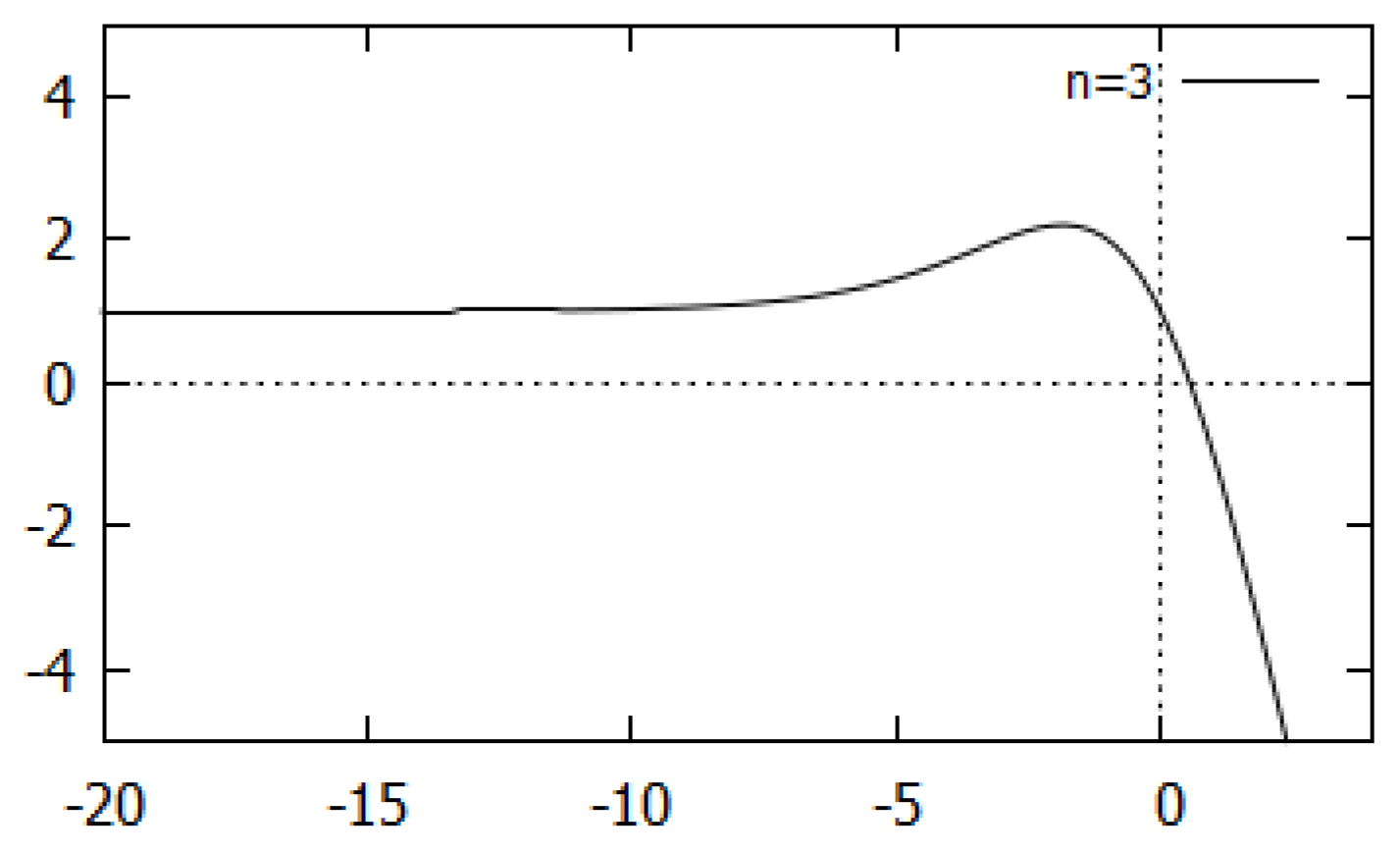
Lemma 1.

Suppose that

$$h\left(x\right)=1-\frac{nx}{1+e^{-x}},x\in \mathbb{R},n\in \mathbb{N}\backslash \left\{1\right\}.$$

Then, the function $h\left(x\right)$ has maximum at $x=\tilde{x}$, where $\tilde{x}$ is the unique negative root of the equation $e^x+x+1=0$.

Moreover, ${\lim }_{x\to -\infty }h\left(x\right)=1$, $h\left(0\right)=1$, ${\lim }_{x\to +\infty }h\left(x\right)=-\infty$, $h\left(x^{*}\right)=-1$, where $x^{*}$ is the unique positive root of the equation $(2-nx)e^x+2=0$ for $n\in \mathbb{N}\backslash \left\{1\right\}$.

Proof. 

Since $h^{\prime }\left(x\right)=-n\frac{1+e^{-x}+x{e}^{-x}}{{(1+e^{-x})}^2}$, then, for extrema, we have $h^{\prime }\left(x\right)=0$. It gives that $e^x+x+1=0$. This equation has only one real root, say $\tilde{x}$. With a brief analysis, it is shown that $h^{\prime \prime }\left(\tilde{x}\right)<0$. Hence $h\left(x\right)$ has maximum at $x=\tilde{x}$.

It is seen that the function $\frac{x}{1+e^{-x}}$ tends to 0 as $x\to -\infty$ and tends to ∞ as $x\to \infty$. Then,

$$\begin{array}{c}\underset{x\to -\infty }{\lim }h\left(x\right)=1-n\underset{x\to -\infty }{\lim }\frac{x}{1+e^{-x}}=1\\ h\left(0\right)=1-n\times 0=1\\ \underset{x\to +\infty }{\lim }h\left(x\right)=1-n\underset{x\to +\infty }{\lim }\frac{x}{1+e^{-x}}=-\infty \\ h\left(x^{*}\right)=1-\frac{n{x}^{*}}{1+e^{-x^{*}}}=1-\frac{n{x}^{*}}{\frac{n{x}^{*}}{2}}=-1\mathrm{since}1+e^{-x^{*}}=\frac{n{x}^{*}}{2}.\end{array}$$

The graph of the function $h\left(x\right)=1-\frac{nx}{1+e^{-x}}$ is given in Figure 1 for $n=3$. ☐

Let us define

$${\lambda }^{*}={(e^{x^{*}}+1)}^n$$

where $x^{*}$ is the unique positive root of the equation $(2-nx)e^x+2=0$ for $n\in \mathbb{N}\backslash \left\{1\right\}$.

The nature of the real fixed points of $f_{\lambda ,n}\left(x\right)$ is explored in the following theorem:

Theorem 2.

Let $f_{\lambda ,n}\in \mathcal{F}$.

(a) 

The fixed point 0 of the function $f_{\lambda ,n}\left(x\right)$ is attracting for $\lambda <2^n$, rationally indifferent for $\lambda =2^n$ and repelling for $\lambda >2^n$.

(b) 

The fixed point $x_{\lambda ,n}$ (negative) of the function $f_{\lambda ,n}\left(x\right)$ is repelling for $1<\lambda <2^n$ and the fixed point $x_{\lambda ,n}$ (positive) of the function $f_{\lambda ,n}\left(x\right)$ is attracting for $2^n<\lambda <{\lambda }^{*}$, rationally indifferent for $\lambda ={\lambda }^{*}$ and repelling for $\lambda >{\lambda }^{*}$.

Proof. 

We have

$$\begin{array}{c}{f}_{\lambda ,n}^{\prime }\left(x\right)=\lambda \frac{(1-nx)e^x+1}{{(e^x+1)}^{n+1}}\end{array}$$

(4)

(a)

For fixed point 0, we obtain $f_{\lambda ,n}^{\prime }\left(0\right)=\frac{\lambda }{2^n}$. Hence, $0<f_{\lambda ,n}^{\prime }\left(0\right)<1$ for $\lambda <2^n$, $f_{\lambda ,n}^{\prime }\left(0\right)=1$ for $\lambda =2^n$ and $f_{\lambda ,n}^{\prime }\left(0\right)>1$ for $\lambda >2^n$. Therefore, it follows that the fixed point 0 of $f_{\lambda ,n}\left(x\right)$ is attracting for $\lambda <2^n$, rationally indifferent for $\lambda =2^n$ and repelling for $\lambda >2^n$.

(b)

For $\lambda >0$ and $x\in \mathbb{R}$, it is easily seen that $f_{\lambda ,n}\left(x\right)>0$ for $x>0$ and $f_{\lambda ,n}\left(x\right)<0$ for $x<0$. Since $x_{\lambda ,n}$ is a fixed point of $f_{\lambda ,n}\left(x\right)$, then, by Equation (4),

$$\begin{array}{c}{f}_{\lambda ,n}^{\prime }\left(x\right)={(e^{x_{\lambda ,n}}+1)}^n\frac{(1-n{x}_{\lambda ,n})e^{x_{\lambda ,n}}+1}{{(e^{x_{\lambda ,n}}+1)}^{n+1}}=1-\frac{n{x}_{\lambda ,n}}{1+e^{-x_{\lambda ,n}}}.\end{array}$$

(5)

The fixed point $x_{\lambda ,n}$ of $f_{\lambda ,n}\left(x\right)$ is negative for $1<\lambda <2^n$ by Theorem 1. By Equation (5), it is seen that, using Lemma 1, $f_{\lambda ,n}^{\prime }\left(x_{\lambda ,n}\right)>1$ for $1<\lambda <2^n$. Hence, the fixed point $x_{\lambda ,n}$ (negative) of the function $f_{\lambda ,n}\left(x\right)$ is repelling for $1<\lambda <2^n$.

The fixed point $x_{\lambda ,n}$ of $f_{\lambda ,n}\left(x\right)$ is positive for $\lambda >2^n$ by Theorem 1. Similarly as above, applying Lemma 1, we have $-1<f_{\lambda ,n}^{\prime }\left(x_{\lambda ,n}\right)<1$ for $2^n<\lambda <{\lambda }^{*}$, $f_{\lambda ,n}^{\prime }\left(x_{\lambda ,n}\right)=-1$ for $\lambda ={\lambda }^{*}$ and $f_{\lambda ,n}^{\prime }\left(x_{\lambda ,n}\right)<-1$ for $\lambda >{\lambda }^{*}$. It follows that the fixed point $x_{\lambda ,n}$ (positive) of $f_{\lambda ,n}\left(x\right)$ is attracting for $2^n<\lambda <{\lambda }^{*}$, rationally indifferent for $\lambda ={\lambda }^{*}$ and repelling for $\lambda >{\lambda }^{*}$.

This completes the proof of theorem. ☐

For $\lambda >{\lambda }^{*}$, there exist periodic points of periods greater than or equal to 2. We discuss these cases in the next section using numerical simulations.

3. Numerical Simulation of Real Periodic Points of $f_{\lambda ,n}\in \mathcal{F}$ and Their Nature

In this section, the numerical simulation of real periodic points of $f_{\lambda ,n}\in \mathcal{F}$ and their nature are discussed since the theoretical computation of the periodic points of $f_{\lambda ,n}\left(x\right)$ is significantly complicated. For $\lambda >{\lambda }^{*}$, the function $f_{\lambda ,n}\left(x\right)$ has periodic points of period greater than or equal to 2 in $(0,\infty )$ in addition to having one fixed point 0 for all $\lambda$ and another nonzero fixed point $x_{\lambda ,n}$ for $\lambda >1$. These periodic points are roots of ${\displaystyle f_{\lambda ,n}^k\left(x\right)\equiv \lambda \frac{f_{\lambda ,n}^{k-1}\left(x\right)}{{(e^{f_{\lambda ,n}^{k-1}\left(x\right)}+1)}^n}=x}$. The periodic cycles of period $2,4,8,16,\dots$ come into existence when parameter $\lambda$ increases beyond ${\lambda }^{*}$. For $n=2$, the periodic points of period 2 start from $\lambda \approx 21.1$.

3.1. Numerical Computation of Real Periodic Points of Period $2,4,8$ and Their Nature

Here, we numerically compute the real periodic points of period $2,4$ and 8 for $n=2,3,4,5$ and their nature.

For $n=2$, the following periodic points of period $2,4,8$ of $f_{\lambda ,n}\left(x\right)$ are computed numerically for different values of parameter $\lambda =22,33,36.5$ respectively:

• If $\lambda =22$, then the 2-cycle periodic points $p_1$ and $p_2$ of $f_{\lambda ,n}\left(x\right)$ are obtained as $p_1\approx 1.01017$ and $p_2\approx 1.58368$. Then, $f_{\lambda ,n}^{\prime }\left(p_1\right)\approx -0.75410$ and $f_{\lambda ,n}^{\prime }\left(p_2\right)\approx -1.03846$. It follows that

  $$|f_{\lambda ,n}^{\prime }\left(p_1\right)f_{\lambda ,n}^{\prime }\left(p_2\right)|\approx 0.78310<1.$$
  Hence, the periodic 2-cycle of $f_{22,2}\left(x\right)$ is attracting.
• If $\lambda =33$, then the 4-cycle periodic points $p_1$, $p_2$, $p_3$ and $p_4$ of $f_{\lambda ,n}\left(x\right)$ are found as $p_1\approx 0.66802$, $p_2\approx 2.53250$, $p_3\approx 0.45284$ and $p_4\approx 2.25765$. Then, $f_{\lambda ,n}^{\prime }\left(p_1\right)\approx 0.442755$, $f_{\lambda ,n}^{\prime }\left(p_2\right)\approx -0.66020$, $f_{\lambda ,n}^{\prime }\left(p_3\right)\approx 2.225257$ and $f_{\lambda ,n}^{\prime }\left(p_4\right)\approx -0.91365$. It follows that

  $$|f_{\lambda ,n}^{\prime }\left(p_1\right)f_{\lambda ,n}^{\prime }\left(p_2\right)f_{\lambda ,n}^{\prime }\left(p_3\right)f_{\lambda ,n}^{\prime }\left(p_4\right)|\approx 0.59429<1.$$
  Consequently, the periodic 4-cycle of $f_{33,2}\left(x\right)$ is attracting.
• If $\lambda =36.5$, then the 8-cycle periodic points $p_1$, $p_2$, $p_3$, $p_4$, $p_5$, $p_6$, $p_7$ and $p_8$ of $f_{\lambda ,n}\left(x\right)$ are determined as $p_1\approx 0.72695$, $p_2\approx 2.81755$, $p_3\approx 0.32694$, $p_4\approx 2.09487$, $p_5\approx 0.91843$, $p_6\approx 2.72820$, $p_7\approx 0.37455$ and $p_8\approx 2.26953$. Then, $f_{\lambda ,n}^{\prime }\left(p_1\right)\approx 0.077016$, $f_{\lambda ,n}^{\prime }\left(p_2\right)\approx -0.50097$, $f_{\lambda ,n}^{\prime }\left(p_3\right)\approx 3.973252$, $f_{\lambda ,n}^{\prime }\left(p_4\right)\approx -1.19712$, $f_{\lambda ,n}^{\prime }\left(p_5\right)\approx -0.92929$, $f_{\lambda ,n}^{\prime }\left(p_6\right)\approx -0.56587$, $f_{\lambda ,n}^{\prime }\left(p_7\right)\approx 3.36965$ and $f_{\lambda ,n}^{\prime }\left(p_8\right)\approx -0.99739$. It follows that

  $$|f_{\lambda ,n}^{\prime }\left(p_1\right)f_{\lambda ,n}^{\prime }\left(p_2\right)f_{\lambda ,n}^{\prime }\left(p_3\right)f_{\lambda ,n}^{\prime }\left(p_4\right)f_{\lambda ,n}^{\prime }\left(p_5\right)f_{\lambda ,n}^{\prime }\left(p_6\right)f_{\lambda ,n}^{\prime }\left(p_7\right)f_{\lambda ,n}^{\prime }\left(p_8\right)|\approx 0.32434<1.$$
  It gives that the periodic 8-cycle of $f_{36.5,2}\left(x\right)$ is attracting.

For $n=3$, the following periodic points of period $2,4,8$ of $f_{\lambda ,n}\left(x\right)$ are determined for different values of parameter $\lambda =46,70,75.5$ respectively:

⋄

If $\lambda =46$, then the 2-cycle periodic points $q_1$ and $q_2$ of $f_{\lambda ,n}\left(x\right)$ are obtained as $q_1\approx 0.73369$ and $q_2\approx 1.15201$. Then, $f_{\lambda ,n}^{\prime }\left(q_1\right)\approx -0.76478$ and $f_{\lambda ,n}^{\prime }\left(q_2\right)\approx -1.03566$. It follows that

$$|f_{\lambda ,n}^{\prime }\left(q_1\right)f_{\lambda ,n}^{\prime }\left(q_2\right)|\approx 0.79205<1.$$

Therefore, the periodic 2-cycle of $f_{46,3}\left(x\right)$ is attracting.

⋄

If $\lambda =70$, then the 4-cycle periodic points $q_1$, $q_2$, $q_3$ and $q_4$ of $f_{\lambda ,n}\left(x\right)$ are found as $q_1\approx 0.30215$, $q_2\approx 1.62401$, $q_3\approx 0.50745$ and $q_4\approx 1.88509$. Then, $f_{\lambda ,n}^{\prime }\left(q_1\right)\approx 2.5735$, $f_{\lambda ,n}^{\prime }\left(q_2\right)\approx -0.95922$, $f_{\lambda ,n}^{\prime }\left(q_3\right)\approx 0.18476$ and $f_{\lambda ,n}^{\prime }\left(q_4\right)\approx -0.6267$. It follows that

$$|f_{\lambda ,n}^{\prime }\left(q_1\right)f_{\lambda ,n}^{\prime }\left(q_2\right)f_{\lambda ,n}^{\prime }\left(q_3\right)f_{\lambda ,n}^{\prime }\left(q_4\right)|\approx 0.28584<1.$$

Hence, the periodic 4-cycle of $f_{70,3}\left(x\right)$ is attracting.

⋄

If $\lambda =75.5$, then the 8-cycle periodic points $q_1$, $q_2$, $q_3$, $q_4$, $q_5$, $q_6$, $q_7$ and $q_8$ of $f_{\lambda ,n}\left(x\right)$ are determined as $q_1\approx 0.23708$, $q_2\approx 1.53525$, $q_3\approx 0.64523$, $q_4\approx 1.98419$, $q_5\approx 0.26455$, $q_6\approx 1.63556$, $q_7\approx 0.53548$ and $q_8\approx 2.03524$. Then, $f_{\lambda ,n}^{\prime }\left(q_1\right)\approx 3.90099$, $f_{\lambda ,n}^{\prime }\left(q_2\right)\approx -1.17236$, $f_{\lambda ,n}^{\prime }\left(q_3\right)\approx -0.82934$, $f_{\lambda ,n}^{\prime }\left(q_4\right)\approx -0.56440$, $f_{\lambda ,n}^{\prime }\left(q_5\right)\approx 3.40632$, $f_{\lambda ,n}^{\prime }\left(q_6\right)\approx -1.01707$, $f_{\lambda ,n}^{\prime }\left(q_7\right)\approx -0.05044$ and $f_{\lambda ,n}^{\prime }\left(q_8\right)\approx -0.51257$. It follows that

$$|f_{\lambda ,n}^{\prime }\left(q_1\right)f_{\lambda ,n}^{\prime }\left(q_2\right)f_{\lambda ,n}^{\prime }\left(q_3\right)f_{\lambda ,n}^{\prime }\left(q_4\right)f_{\lambda ,n}^{\prime }\left(q_5\right)f_{\lambda ,n}^{\prime }\left(q_6\right)f_{\lambda ,n}^{\prime }\left(q_7\right)f_{\lambda ,n}^{\prime }\left(q_8\right)|\approx 0.19175<1.$$

It shows that the periodic 8-cycle of $f_{75.5,3}\left(x\right)$ is attracting.

For $n=4$, the following periodic points of period $2,4,8$ of $f_{\lambda ,n}\left(x\right)$ are simulated numerically for different values of parameter $\lambda =110,150,157$ respectively:

○

If $\lambda =110$, then the 2-cycle periodic points $r_1$ and $r_2$ of $f_{\lambda ,n}\left(x\right)$ are obtained as $r_1\approx 0.0.43129$ and $r_2\approx 1.14116$. Then, $f_{\lambda ,n}^{\prime }\left(r_1\right)\approx -0.12111$ and $f_{\lambda ,n}^{\prime }\left(r_2\right)\approx -0.92955$. It follows that

$$|f_{\lambda ,n}^{\prime }\left(r_1\right)f_{\lambda ,n}^{\prime }\left(r_2\right)|\approx 0.11258<1.$$

It gives that the periodic 2-cycle of $f_{110,4}\left(x\right)$ is attracting.

○

If $\lambda =150$, then the 4-cycle periodic points $r_1$, $r_2$, $r_3$ and $r_4$ of $f_{\lambda ,n}\left(x\right)$ are found as $r_1\approx 0.21480$, $r_2\approx 1.28064$, $r_3\approx 0.42942$ and $r_4\approx 1.55642$. Then, $f_{\lambda ,n}^{\prime }\left(r_1\right)\approx 3.12683$, $f_{\lambda ,n}^{\prime }\left(r_2\right)\approx -1.00887$, $f_{\lambda ,n}^{\prime }\left(r_3\right)\approx -0.14664$ and $f_{\lambda ,n}^{\prime }\left(r_4\right)\approx -0.57154$. It follows that

$$|f_{\lambda ,n}^{\prime }\left(r_1\right)f_{\lambda ,n}^{\prime }\left(r_2\right)f_{\lambda ,n}^{\prime }\left(r_3\right)f_{\lambda ,n}^{\prime }\left(r_4\right)|\approx 0.26439<1.$$

Hence, the periodic 4-cycle of $f_{150,4}\left(x\right)$ is attracting.

○

If $\lambda =157$, then the 8-cycle periodic points $r_1$, $r_2$, $r_3$, $r_4$, $r_5$, $r_6$, $r_7$ and $r_8$ of $f_{\lambda ,n}\left(x\right)$ are determined as $r_1\approx 0.42190$, $r_2\approx 1.62991$, $r_3\approx 0.18441$, $r_4\approx 1.23029$, $r_5\approx 0.50506$, $r_6\approx 1.59082$, $r_7\approx 0.20503$ and $r_8\approx 1.30738$. Then, $f_{\lambda ,n}^{\prime }\left(r_1\right)\approx -0.07420$, $f_{\lambda ,n}^{\prime }\left(r_2\right)\approx -0.50363$, $f_{\lambda ,n}^{\prime }\left(r_3\right)\approx 3.9848$, $f_{\lambda ,n}^{\prime }\left(r_4\right)\approx -1.15288$, $f_{\lambda ,n}^{\prime }\left(r_5\right)\approx -0.81868$, $f_{\lambda ,n}^{\prime }\left(r_6\right)\approx -0.55243$, $f_{\lambda ,n}^{\prime }\left(r_7\right)\approx 3.49452$ and $f_{\lambda ,n}^{\prime }\left(r_8\right)\approx -1.00556$. It follows that

$$|f_{\lambda ,n}^{\prime }\left(r_1\right)f_{\lambda ,n}^{\prime }\left(r_2\right)f_{\lambda ,n}^{\prime }\left(r_3\right)f_{\lambda ,n}^{\prime }\left(r_4\right)f_{\lambda ,n}^{\prime }\left(r_5\right)f_{\lambda ,n}^{\prime }\left(r_6\right)f_{\lambda ,n}^{\prime }\left(r_7\right)f_{\lambda ,n}^{\prime }\left(r_8\right)|\approx 0.27283<1.$$

Therefore, it is shown that the periodic 8-cycle of $f_{157,4}\left(x\right)$ is attracting.

For $n=5$, the following periodic points of period $2,4,8$ of $f_{\lambda ,n}\left(x\right)$ are computed for different values of parameter $\lambda =250,300,326$ respectively:

*

If $\lambda =250$, then the 2-cycle periodic points $s_1$ and $s_2$ of $f_{\lambda ,n}\left(x\right)$ are obtained as $s_1\approx 0.30730$ and $s_2\approx 1.04996$. Then, $f_{\lambda ,n}^{\prime }\left(s_1\right)\approx 0.39167$ and $f_{\lambda ,n}^{\prime }\left(s_2\right)\approx -0.84551$. It follows that

$$|f_{\lambda ,n}^{\prime }\left(s_1\right)f_{\lambda ,n}^{\prime }\left(s_2\right)|\approx 0.33116<1.$$

Therefore, the periodic 2-cycle of $f_{250,5}\left(x\right)$ is attracting.

*

If $\lambda =300$, then the 4-cycle periodic points $s_1$, $s_2$, $s_3$ and $s_4$ of $f_{\lambda ,n}\left(x\right)$ are found as $s_1\approx 0.32153$, $s_2\approx 1.26519$, $s_3\approx 0.19598$ and $s_4\approx 1.09897$. Then, $f_{\lambda ,n}^{\prime }\left(s_1\right)\approx 0.26777$, $f_{\lambda ,n}^{\prime }\left(s_2\right)\approx -0.60932$, $f_{\lambda ,n}^{\prime }\left(s_3\right)\approx 2.59193$ and $f_{\lambda ,n}^{\prime }\left(s_4\right)\approx -0.91327$. It follows that

$$|f_{\lambda ,n}^{\prime }\left(s_1\right)f_{\lambda ,n}^{\prime }\left(s_2\right)f_{\lambda ,n}^{\prime }\left(s_3\right)f_{\lambda ,n}^{\prime }\left(s_4\right)|\approx 0.38622<1.$$

Hence, the periodic 4-cycle of $f_{300,5}\left(x\right)$ is attracting.

*

If $\lambda =326$, then the 8-cycle periodic points $s_1$, $s_2$, $s_3$, $s_4$, $s_5$, $s_6$, $s_7$ and $s_8$ of $f_{\lambda ,n}\left(x\right)$ are determined as $s_1\approx 0.42288$, $s_2\approx 1.33958$, $s_3\approx 0.16831$, $s_4\approx 1.10601$, $s_5\approx 0.34247$, $s_6\approx 1.37777$, $s_7\approx 0.14871$ and $s_8\approx 1.03027$. Then, $f_{\lambda ,n}^{\prime }\left(s_1\right)\approx -0.87890$, $f_{\lambda ,n}^{\prime }\left(s_2\right)\approx -0.54122$, $f_{\lambda ,n}^{\prime }\left(s_3\right)\approx 3.57407$, $f_{\lambda ,n}^{\prime }\left(s_4\right)\approx -0.97699$, $f_{\lambda ,n}^{\prime }\left(s_5\right)\approx -0.00549$, $f_{\lambda ,n}^{\prime }\left(s_6\right)\approx -0.48589$, $f_{\lambda ,n}^{\prime }\left(s_7\right)\approx 4.16123$ and $f_{\lambda ,n}^{\prime }\left(s_8\right)\approx -1.14778$. It follows that

$$|f_{\lambda ,n}^{\prime }\left(s_1\right)f_{\lambda ,n}^{\prime }\left(s_2\right)f_{\lambda ,n}^{\prime }\left(s_3\right)f_{\lambda ,n}^{\prime }\left(s_4\right)f_{\lambda ,n}^{\prime }\left(s_5\right)f_{\lambda ,n}^{\prime }\left(s_6\right)f_{\lambda ,n}^{\prime }\left(s_7\right)f_{\lambda ,n}^{\prime }\left(s_8\right)|\approx 0.02115<1.$$

Therefore, it is shown that the periodic 8-cycle of $f_{326,5}\left(x\right)$ is attracting.

3.2. Numerical Computation of Real Periodic Points of Period 3 and Their Nature

We numerically compute the real periodic points of period 3 for $n=2,3,4,5$ corresponding to $\lambda =54,108,229,479$ respectively and their nature.

• For $n=2$ and $\lambda =54$, the 3-cycle periodic points $p_1$, $p_2$ and $p_3$ of $f_{\lambda ,n}\left(x\right)$ are determined as $p_1\approx 0.68468$, $p_2\approx 4.15465$, and $p_3\approx 0.05354$. Then, $f_{\lambda ,n}^{\prime }\left(p_1\right)\approx 0.54416$, $f_{\lambda ,n}^{\prime }\left(p_2\right)\approx -0.09255$ and $f_{\lambda ,n}^{\prime }\left(p_3\right)\approx 12.08398$. It follows that

  $$|f_{\lambda ,n}^{\prime }\left(p_1\right)f_{\lambda ,n}^{\prime }\left(p_2\right)f_{\lambda ,n}^{\prime }\left(p_3\right)|\approx 0.60855<1.$$
  Consequently, the periodic 3-cycle of $f_{54,2}\left(x\right)$ is attracting.
• For $n=3$ and $\lambda =108$, the 3-cycle periodic points $q_1$, $q_2$ and $q_3$ of $f_{\lambda ,n}\left(x\right)$ are computed as $q_1\approx 0.04340$, $q_2\approx 0.54863$, and $q_3\approx 2.90935$. Then, $f_{\lambda ,n}^{\prime }\left(q_1\right)\approx -0.10856$, $f_{\lambda ,n}^{\prime }\left(q_2\right)\approx 11.79935$ and $f_{\lambda ,n}^{\prime }\left(q_3\right)\approx -0.22903$. It follows that

  $$|f_{\lambda ,n}^{\prime }\left(q_1\right)f_{\lambda ,n}^{\prime }\left(q_2\right)f_{\lambda ,n}^{\prime }\left(q_3\right)|\approx 0.29338<1.$$
  Hence, the periodic 3-cycle of $f_{108,3}\left(x\right)$ is attracting.
• For $n=4$ and $\lambda =229$, the 3-cycle periodic points $r_1$, $r_2$ and $r_3$ of $f_{\lambda ,n}\left(x\right)$ are calculated as $r_1\approx 0.02880$, $r_2\approx 0.38893$ and $r_3\approx 2.37205$. Then, $f_{\lambda ,n}^{\prime }\left(r_1\right)\approx 12.71683$, $f_{\lambda ,n}^{\prime }\left(r_2\right)\approx 0.44378$ and $f_{\lambda ,n}^{\prime }\left(r_3\right)\approx -0.09322$. It follows that

  $$|f_{\lambda ,n}^{\prime }\left(r_1\right)f_{\lambda ,n}^{\prime }\left(r_2\right)f_{\lambda ,n}^{\prime }\left(r_3\right)|\approx 0.52608<1.$$
  It shows that the periodic 3-cycle of $f_{229,4}\left(x\right)$ is attracting.
• For $n=5$ and $\lambda =479$, the 3-cycle periodic points $s_1$, $s_2$ and $s_3$ of $f_{\lambda ,n}\left(x\right)$ are simulated as $s_1\approx 0.30982$, $s_2\approx 2.01355$ and $s_3\approx 0.02187$. Then, $f_{\lambda ,n}^{\prime }\left(s_1\right)\approx 0.69152$, $f_{\lambda ,n}^{\prime }\left(s_2\right)\approx -0.08560$ and $f_{\lambda ,n}^{\prime }\left(s_3\right)\approx 13.38513$. It follows that

  $$|f_{\lambda ,n}^{\prime }\left(s_1\right)f_{\lambda ,n}^{\prime }\left(s_2\right)f_{\lambda ,n}^{\prime }\left(s_3\right)|\approx 0.79232<1.$$
  It gives that the periodic 3-cycle of $f_{479,5}\left(x\right)$ is attracting.

We can easily observe the existence of periodic points of periods greater than or equal to 2 in the next section through bifurcation diagrams.

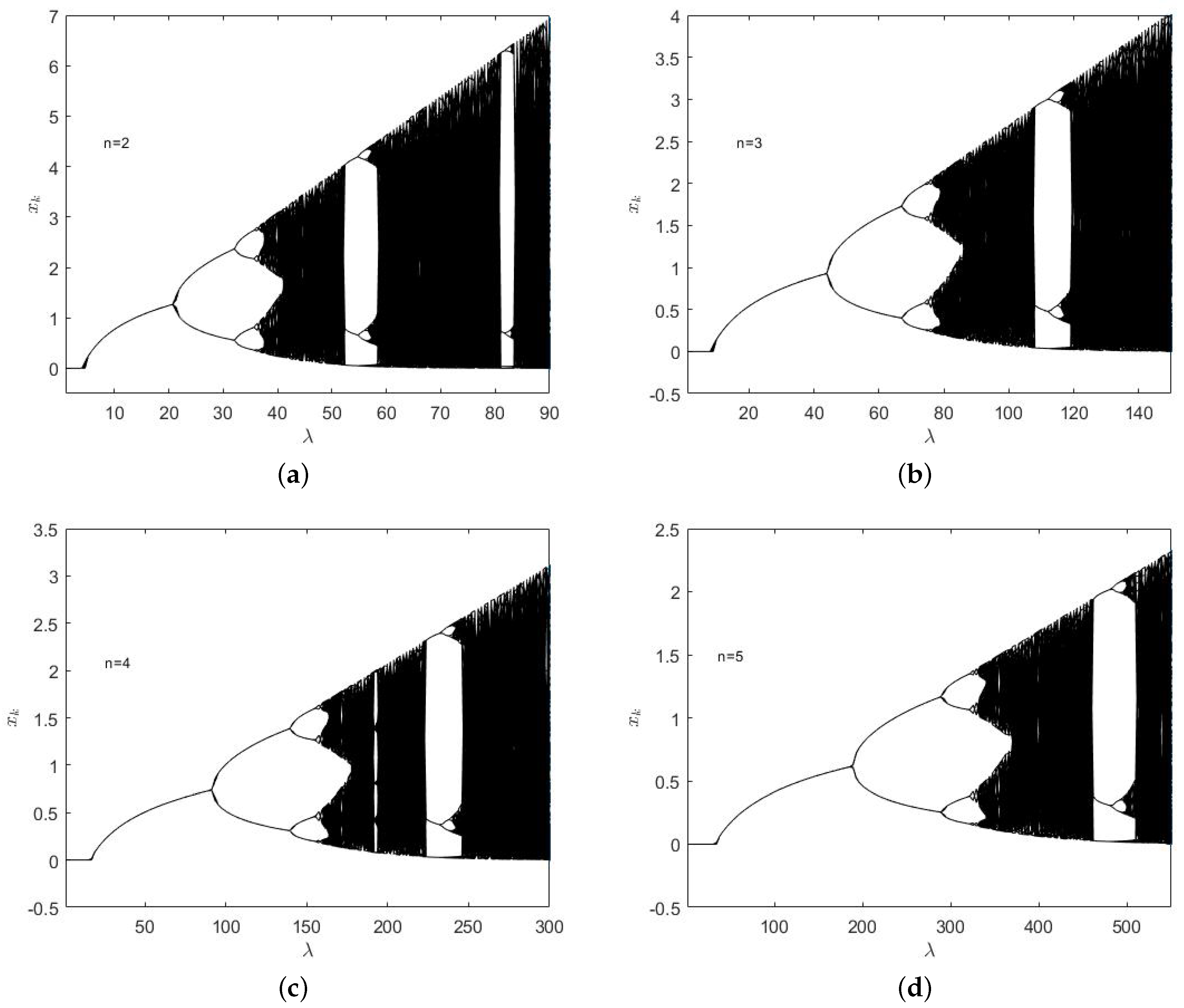
4. Bifurcation Diagrams and Route to Chaos

Using graphical simulation, we explore the dynamical behaviour of $f_{\lambda ,n}\in \mathcal{F}$ through plots of bifurcation diagrams in this section. It is known that if the period-doubling occurs in the real dynamics of function, then it is a route to chaos in the real dynamics of function and period 3 implies chaos [1]. From Theorem 2, it is observed that the nature of the fixed points of $f_{\lambda ,n}\left(x\right)$ changes when parameter $\lambda$ crosses a certain parameter value. Further, if the parameter $\lambda$ increases, then the periodic points of period 2 or more occur in the dynamical system. It can be seen by bifurcation diagrams in Figure 2 for $n=2,3,4,5$ with $1\le \lambda \le 90$, $1\le \lambda \le 150$, $1\le \lambda \le 300$ and $1\le \lambda \le 550$ respectively. It is easily seen that the period-doubling occurs in these bifurcation diagrams. Moreover, period 3 is also visible in these bifurcation diagrams.

In bifurcation diagrams (Figure 2a–d), it is observed that when n increases from 2 to 5, then the period-doubling happens for larger values of parameter $\lambda$. The occurrence of periodic-doubling in the bifurcation diagrams leads to a route to chaos in the real dynamics of $f_{\lambda ,n}\in \mathcal{F}$. Moreover, white regions represent the appearance of periodic windows inside bifurcation diagrams. It is also seen that a periodic 3-window also occurs in the bifurcation diagrams of $f_{\lambda ,n}\left(x\right)$ for $n=2,3,4,5$ corresponding to $\lambda =54,108,229,479$ respectively which also represents chaotic behaviour in the dynamical system. After this periodic 3-window, a new 6-period cycle comes into existence. After that, we enter into a very complicated dynamics region.

In the next section, Lyapunov exponents are computed corresponding to values of parameter $\lambda$ for which period-doubling happens in the bifurcation diagrams.

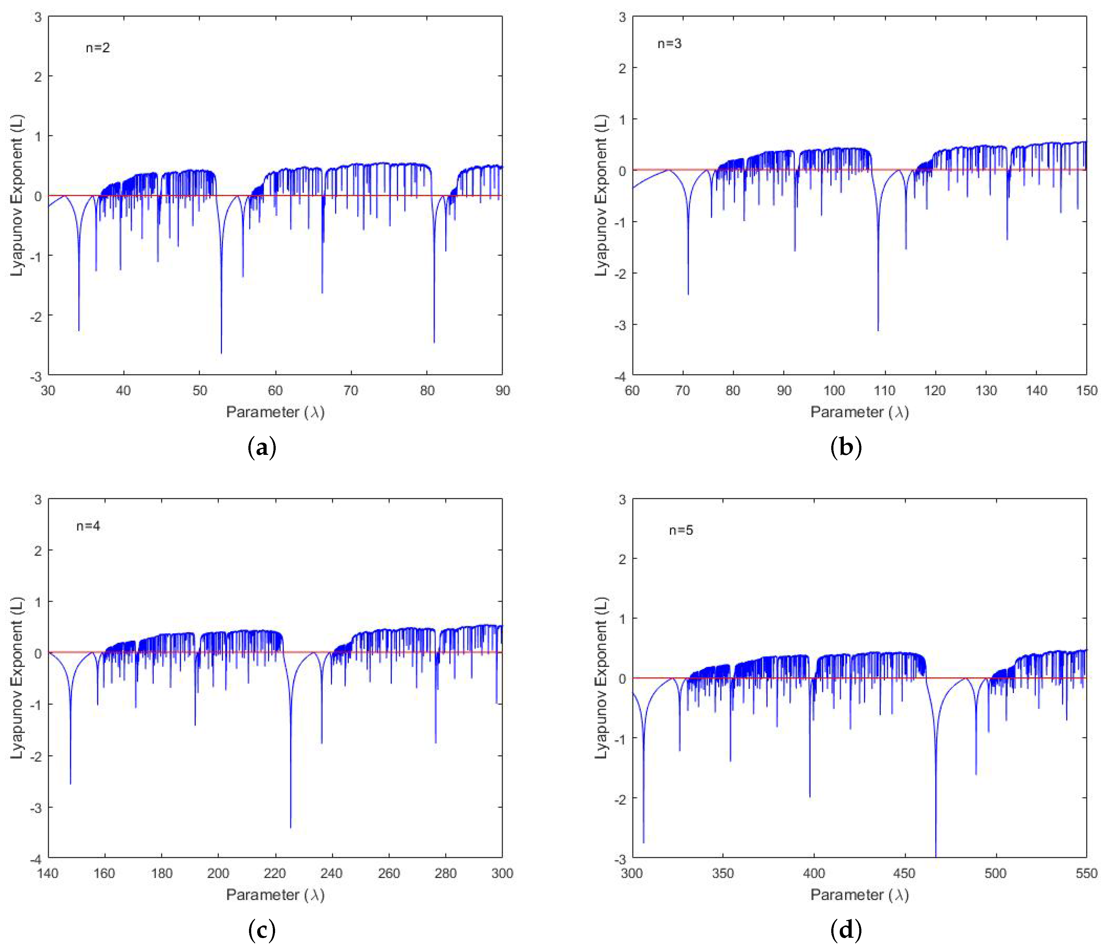
5. Lyapunov Exponents

To quantify the chaos, the Lyapunov exponent of the function $f_{\lambda ,n}\in \mathcal{F}$ needs to be computed which is the main key for the chaotic systems. It is known that if the Lyapunov exponent is positive, then it represents chaotic behaviour in the dynamical system [1]. Using Formula (1), the Lyapunov exponent of the function $f_{\lambda ,n}\in \mathcal{F}$ is computed as

$$L=\underset{k\to \infty }{\lim }\frac{1}{k}\sum _{i=0}^{k-1}\ln \left[\lambda \frac{|(1-n{x}_i)e^{x_i}+1|}{{(e^{x_i}+1)}^{n+1}}\right].$$

For our computation, we choose $x_0=0.5$ and $k=5000$. The computed values of Lyapunov exponents are demonstrated in Figure 3 for $n=2,3,4,5$ with $30\le \lambda \le 90$, $60\le \lambda \le 150$, $140\le \lambda \le 300$ and $300\le \lambda \le 550$ respectively. From these figures, it is observed that the Lyapunov exponents are positive for certain ranges of parameter $\lambda$ which exhibits sensitive dependence on the initial conditions. Hence, the chaotic behaviour exists in the real dynamics of $f_{\lambda ,n}\in \mathcal{F}$.

The bifurcation diagrams in Figure 2 and the corresponding Lyapunov exponents L in Figure 3, for intervals of parameter $\lambda$, are represented as follows: when Lyapunov exponents are positive, then the bifurcation diagrams have dark regions which show chaotic behaviour in the real dynamics $f_{\lambda ,n}\left(x\right)$ for certain ranges of parameter values. Moreover, for some ranges, Lyapunov exponents are negative and bifurcation diagrams have white regions; this shows that the chaotic regions break up into non-chaotic temporarily and then return to being chaotic.

6. Conclusions

In the present paper, the bifurcation and chaotic behaviour have been determined in the real dynamics of the two-parameter family of transcendental functions; this family of functions arises from the generating function of the generalized Apostol-type polynomials. The real fixed points of these transcendental functions and their stability have been obtained analytically while the periodic points of these functions have been computed numerically. The existence of chaotic behaviour has been observed by periodic doubling and it has been exhibited by bifurcation diagrams. Chaos in the real dynamics has been quantified by computing positive Lyapunov exponents. The following are possible future research directions: Such results could also be obtained for other kinds of generating functions. Moreover, such results could be extended for a family of functions involving three-parameter values as well as for a family of functions in two or more dimensions.

References

1. Gulick, D. Encounters with Chaos and Fractals, 2nd ed.; Chapman and Hall/CRC: Boca Raton, FL, USA, 2012. [Google Scholar]
2. Thunberg, H. Periodicity versus chaos in one-dimensional dynamics. SIAM Rev. 2001, 43, 3–30. [Google Scholar] [CrossRef]
3. Stavroulaki, M.; Sotiropoulos, D. The energy of generalized logistic maps at full chaos. Chaotic Model. Simul. 2012, 3, 543–550. [Google Scholar]
4. Radwan, A.G. On some generalized discrete logistic maps. J. Adv. Res. 2013, 4, 163–171. [Google Scholar] [CrossRef]
5. Akbari, M.; Rabii, M. Real cubic polynomials with a fixed point of multiplicity two. Indagat. Math. 2015, 26, 64–74. [Google Scholar] [CrossRef]
6. Magrenan, A.; Gutierrez, J. Real dynamics for damped Newton’s method applied to cubic polynomials. J. Comput. Appl. Math. 2015, 275, 527–538. [Google Scholar] [CrossRef]
7. Yang, X.S. Applied Engineering Mathematics; Cambridge International Science Publishing: Cambridge, UK, 2007. [Google Scholar]
8. Ozer, M.; Cenys, A.; Polatoglu, Y.; Hacibekiroglu, G.; Akat, E.; Valaristos, A.; Anagnostopoulos, A.N. Bifurcations of Fibonacci generating functions. Chaos Solitons Fractals 2014, 33, 1240–1247. [Google Scholar] [CrossRef]
9. Kumar, P.; Miller, N. Chaotic dynamics of one-dimensional systems with periodic boundary conditions. Phys. Rev. E 2014, 90. [Google Scholar] [CrossRef] [PubMed]
10. Lim, D. Fixed points and dynamics on generating function of Genocchi numbers. J. Nonlinear Sci. Appl. 2016, 9, 933–939. [Google Scholar] [CrossRef]
11. De Carvalho, R.E.; Leonel, E.D. Squared sine logistic map. Physics A 2016, 463, 37–44. [Google Scholar] [CrossRef]
12. Sajid, M.; Alsuwaiyan, A.S. Chaotic behavior in the real dynamics of a one parameter family of functions. Int. J. Appl. Sci. Eng. 2014, 12, 283–301. [Google Scholar]
13. Sajid, M. Real fixed points and dynamics of one parameter family of function (bx−1)/x. J. Assoc. Arab Univ. Basic Appl. Sci. 2016, 21, 92–95. [Google Scholar] [CrossRef]
14. Magrenan, A.A. A new tool to study real dynamics: The convergence plane. Appl. Math. Comput. 2014, 248, 215–224. [Google Scholar] [CrossRef]
15. Sajid, M. On fixed points of one parameter family of function x b x 1 II. Int. J. Math. Anal. 2014, 8, 891–894. [Google Scholar] [CrossRef]
16. Sajid, M. On real fixed points of one parameter family of function x b x 1 . Tamkang J. Math. 2015, 46, 61–65. [Google Scholar] [CrossRef]
17. Sajid, M. Singular values and fixed points of family of generating function of Bernoulli’s numbers. J. Nonlinear Sci. Appl. 2015, 8, 17–22. [Google Scholar] [CrossRef]
18. Lee, M.G.; Ho, C.C. Fixed points of two-parameter family of function λ( x b x 1 )n. Appl. Math. 2015, 6, 576–584. [Google Scholar] [CrossRef]
19. Sajid, M. Real fixed points and singular values of two-parameter family λz/(ez−1)n. New Trends Math. Sci. 2017, 5, 107–113. [Google Scholar] [CrossRef]
20. Devaney, R.L. Sex: Dynamics, topology, and bifurcations of complex exponentials. Topol. Appl. 2001, 110, 133–161. [Google Scholar] [CrossRef]
21. Kapoor, G.P.; Prasad, M.G.P. Dynamics of (ez−1)/z: The Julia set and bifurcation. Ergod. Theory Dyn. Syst. 1998, 18, 1363–1383. [Google Scholar] [CrossRef]
22. Nayak, T.; Prasad, M.G.P. Julia sets of Joukowski-Exponential maps. Complex Anal. Oper. Theory 2014, 8, 1061–1076. [Google Scholar] [CrossRef]
23. Sajid, M.; Kapoor, G.P. Dynamics of transcendental meromorphic functions ( z + μ 0 ) ( z + μ 0 + 4 ) ez having rational Schwarzian derivative. Dyn. Syst. Int. J. 2007, 22, 323–337. [Google Scholar] [CrossRef]
24. Sharifi, S.; Salimi, M.; Siegmund, S.; Lotfi, T. A new class of optimal four-point methods with convergence order 16 for solving nonlinear equations. Math. Comput. Simul. 2016, 119, 69–90. [Google Scholar] [CrossRef]
25. Sajid, M.; Kapoor, G.P. Chaos in dynamics of a family of transcendental meromorphic functions. J. Nonlinear Anal. Appl. 2017, 2017, 1–11. [Google Scholar] [CrossRef]
26. Chakra, T.K.; Nayak, T. Iteration of the Translated Tangent. Bull. Malays. Math. Sci. Soc. 2017. [Google Scholar] [CrossRef]
27. Florian, S. Mechanics: From Newton’s Laws to Deterministic Chaos, 5th ed.; Springer: Berlin, Germany, 2010. [Google Scholar]
28. Kapitaniak, T. Chaos for Engineers: Theory Applications and Control, 2nd ed.; Springer: Berlin, Germany, 2000. [Google Scholar]
29. Thompson, J.M.T.; Stewart, H.B. Nonlinear Dynamics and Chaos; John Wiley & Sons: Hoboken, NJ, USA, 2002. [Google Scholar]
30. Kautz, R. Chaos; Oxford University Press: Oxford, UK, 2011. [Google Scholar]
31. Pikovsky, A.; Politi, A. Lyapunov Exponents: A Tool to Explore Complex Dynamics; Cambridge University Press: Cambridge, UK, 2016. [Google Scholar]
32. Luo, Q.M.; Srivastava, H.M. Some generalizations of the Apostol-Genocchi polynomials and the Stirling numbers of the second kind. Appl. Math. Comput. 2011, 217, 5702–5728. [Google Scholar] [CrossRef]
Figure 1. Graph of h ( x ) = 1 n x 1 + e x for n = 3 .
Mca 23 00007 g001
Figure 2. Bifrucation diagrams for (a) n = 2 ; (b) n = 3 ; (c) n = 4 ; (d) n = 5 .
Mca 23 00007 g002
Figure 3. Lyapunov exponents for (a) n = 2 ; (b) n = 3 ; (c) n = 4 ; (d) n = 5 .
Mca 23 00007 g003