A Survey of Recent Trends in Multiobjective Optimal Control—Surrogate Models, Feedback Control and Objective Reduction


Abstract
1. Introduction
2. Multiobjective Optimization
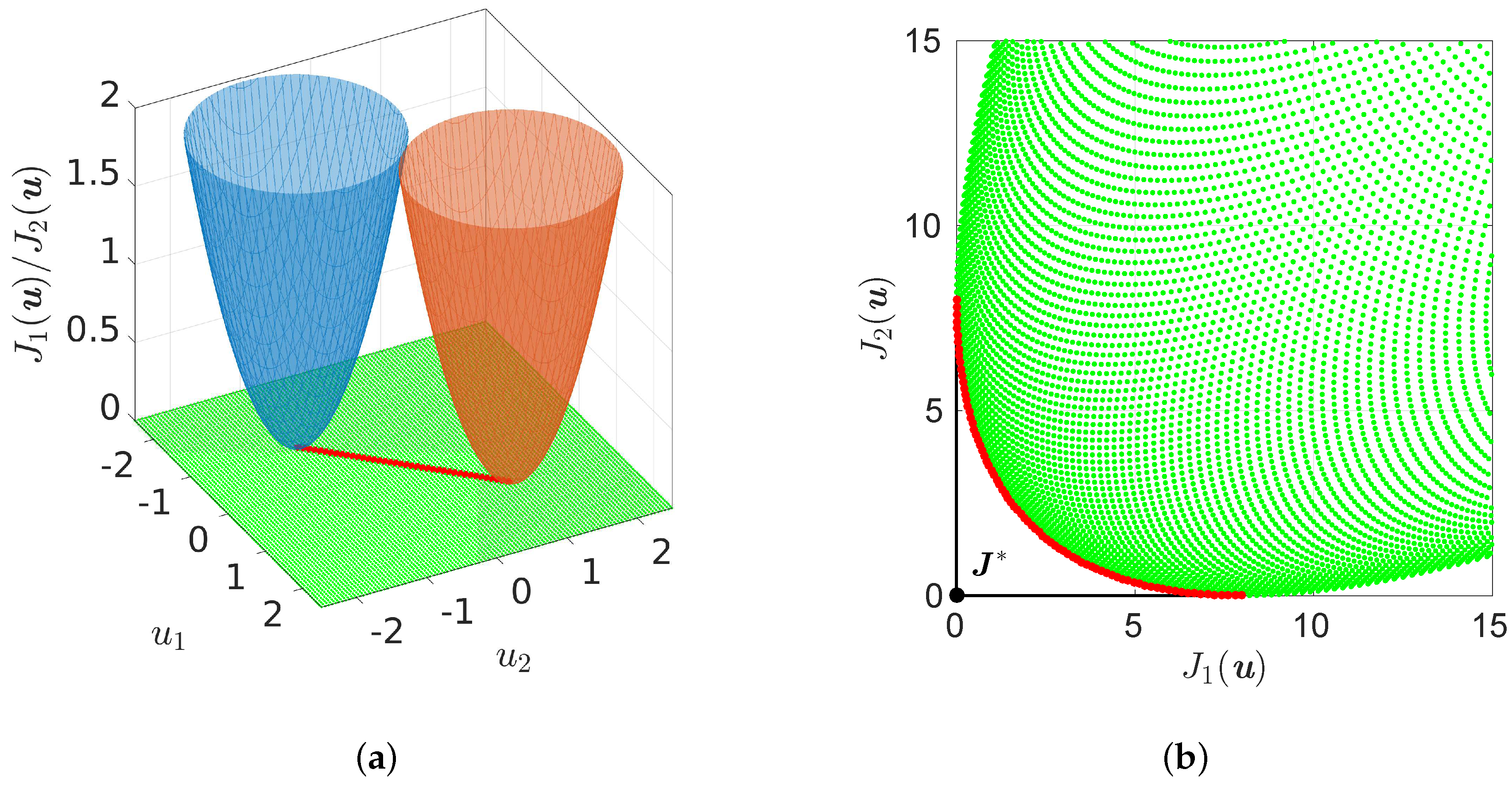
2.1. Theory
- 1.
- a point dominates a point u, if and .
- 2.
- a feasible point is called globally Pareto optimal if there exists no feasible point dominating . The image of a globally Pareto optimal point is called a globally Pareto optimal value. If this property holds in a neighborhood , then is called locally Pareto optimal.
- 3.
- the set of non-dominated feasible points is called the Pareto set and its image the Pareto front .
2.2. Solution Methods
3. Surrogate Models
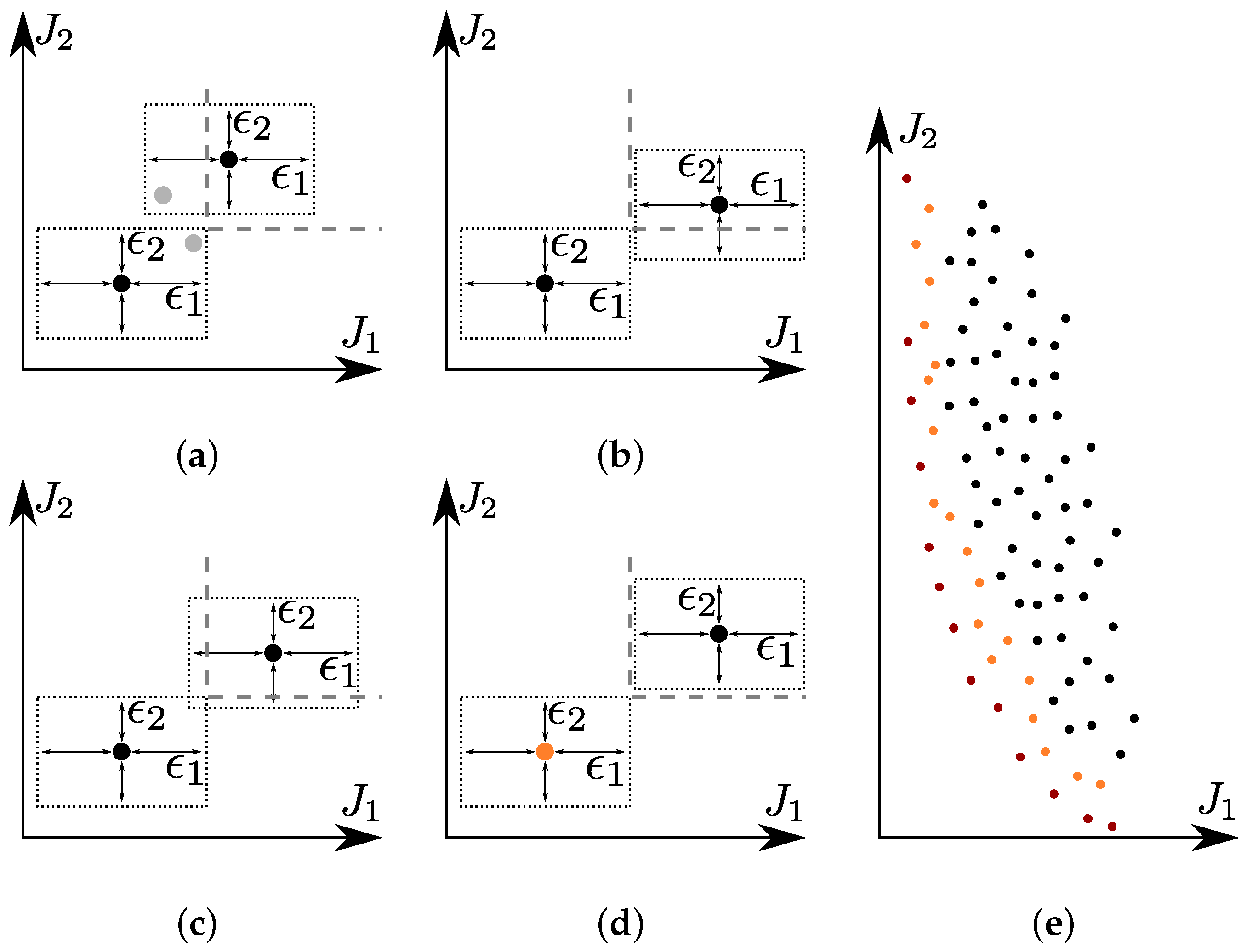
3.1. Inaccuracies and -Dominance
- 1.
- a point confidently dominates a point u, if and for at least one .
- 2.
- The set of almost non-dominated points, which is a superset of the Pareto set , is defined as:
- (a)
- If then there exists no direction with:i.e., no descent direction for the exact problem.
- (b)
- All points u with are contained in the set:
3.2. Surrogate Models for the Objective Function
- Response Surface Models (RSM);
- Radial Basis Functions (RBF);
- statistical models such as Kriging or Gauss regression;
- machine learning methods such as artificial neural networks or support vector machines;
- How large does the set have to be?
- How can we pick the correct elements for ?
- Do we define in advance or online during the model building process?
3.3. Surrogate Models for the Dynamical System
3.3.1. ROMS via Proper Orthogonal Decomposition or the Reduced Basis Method
3.3.2. Optimal Control Using Surrogate Models
- build a model once,
- construction of regular updates in a trust region approach,
- construction of regular updates using error estimators.
3.4. ROM-Based Multiobjective Optimal Control of PDEs
3.4.1. Scalarization
3.4.2. Set-Oriented Approaches with -Dominance
3.5. Summary
4. Feedback Control
4.1. Online Multiobjective Optimization
- compute a single Pareto-optimal solution according to some predefined preference,
- compute only a rough approximation of the Pareto set,
- compute an arbitrary Pareto-optimal control that satisfies additional constraints (e.g., stability).
4.2. Offline-Online Decomposition
4.2.1. Example: Autonomous Driving
4.3. Summary
5. Reduction Techniques for Many-Objective Optimization Problems
6. Future Directions
Author Contributions
Acknowledgments
Conflicts of Interest
References
- Knowles, J.; Nakayama, H. Meta-Modeling in Multiobjective Optimization. In Multiobjective Optimization: Interactive and Evolutionary Approaches; Branke, J., Deb, K., Miettinen, K., Slowinski, R., Eds.; Springer: Berlin/Heidelberg, Germany, 2008; pp. 245–284. [Google Scholar]
- Tabatabaei, M.; Hakanen, J.; Hartikainen, M.; Miettinen, K.; Sindhya, K. A survey on handling computationally expensive multiobjective optimization problems using surrogates: Non-nature inspired methods. Struct. Multidiscip. Optim. 2015, 52, 1–25. [Google Scholar] [CrossRef]
- Chugh, T.; Sindhya, K.; Hakanen, J.; Miettinen, K. A survey on handling computationally expensive multiobjective optimization problems with evolutionary algorithms. Soft Comput. 2017, 1–30. [Google Scholar] [CrossRef]
- Miettinen, K. Nonlinear Multiobjective Optimization; Springer Science and Business Media: Berlin, Germany, 2012. [Google Scholar]
- Ehrgott, M. Multicriteria Optimization, 2nd ed.; Springer: Berlin/Heidelberg, Germany; New York, NY, USA, 2005. [Google Scholar]
- Hindi, H.A.; Hassibi, B.; Boyd, S.B. Multiobjective 2/∞-Optimal Control via Finite Dimensional Q-Parametrization and Linear Matrix Inequalities. In Proceedings of the American Control Conference, Philadelphia, PA, USA, 24–26 June 1998; pp. 3244–3249. [Google Scholar]
- Zhu, Q.J. Hamiltonian Necessary Conditions for a Multiobjective Optimal Control Problem with Endpoint Constraints. SIAM J. Control Optim. 2000, 39, 97–112. [Google Scholar] [CrossRef]
- Gambier, A.; Badreddin, E. Multi-objective optimal control: An overview. In Proceedings of the 16th IEEE International Conference on Control Applciations, Singapore, 1–3 October 2007; pp. 170–175. [Google Scholar]
- Tröltzsch, F. Optimal Control Of Partial Differential Equations. In Graduate Studies in Mathematics; American Mathematical Society: Providence, RI, USA, 2010; Volume 112. [Google Scholar]
- Hinze, M.; Pinnau, R.; Ulbrich, M.; Ulbrich, S. Optimization with PDE Constraints; Springer Science+Business Media: Berlin, Germany, 2009. [Google Scholar]
- Ober-Blöbaum, S. Discrete Mechanics and Optimal Control. Ph.D. Thesis, University of Paderborn, Paderborn, Germany, 2008. [Google Scholar]
- Schilders, W.H.A.; van der Vorst, H.A.; Rommes, J. Model Order Reduction; Springer: Berlin/Heidelberg, Germany, 2008. [Google Scholar]
- Karush, W. Minima of Functions of Several Variables with Inequalities as Side Constraints. Master’s Thesis, University of Chicago, Chicago, IL, USA, 1939. [Google Scholar]
- Kuhn, H.W.; Tucker, A.W. Nonlinear programming. In Proceedings of the 2nd Berkeley Symposium on Mathematical and Statsitical Probability, Oakland, CA, USA, 31 July–12 August 1950; University of California Press: Berkeley, CA, USA, 1951; pp. 481–492. [Google Scholar]
- Romaus, C.; Böcker, J.; Witting, K.; Seifried, A.; Znamenshchykov, O. Optimal energy management for a hybrid energy storage system combining batteries and double layer capacitors. In Proceedings of the IEEE Energy Conversion Congress and Exposition, San Jose, CA, USA, 20–24 September 2009; pp. 1640–1647. [Google Scholar]
- Hillermeier, C. Nonlinear Multiobjective Optimization: A Generalized Homotopy Approach; Birkhäuser: Basel, Switzerland, 2001. [Google Scholar]
- Schütze, O.; Dell’Aere, A.; Dellnitz, M. On Continuation Methods for the Numerical Treatment of Multi-Objective Optimization Problems. Available online: http://drops.dagstuhl.de/opus/volltexte/2005/349/pdf/04461.SchuetzeOliver.Paper.349.pdf (accessed on 31 May 2018).
- Deb, K. Multi-Objective Optimization Using Evolutionary Algorithms; John Wiley and Sons: Hoboken, NJ, USA, 2001; Volume 16. [Google Scholar]
- Coello Coello, C.A.; Lamont, G.B.; Van Veldhuizen, D.A. Evolutionary Algorithms for Solving Multi-Objective Problems; Springer Science and Business Media: Berlin, Germany, 2007; Volume 2. [Google Scholar]
- Zitzler, E.; Laumanns, M.; Thiele, L. SPEA2: Improving the Strength Pareto Evolutionary Algorithm. Available online: https://www.research-collection.ethz.ch/bitstream/handle/20.500.11850/145755/eth-24689-01.pdf (accessed on 31 May 2018).
- Deb, K.; Pratap, A.; Agarwal, S.; Meyarivan, T. A Fast and Elitist Multiobjective Genetic Algorithm: NSGA-II. IEEE Trans. Evol. Comput. 2002, 6, 182–197. [Google Scholar] [CrossRef]
- Zhou, A.; Qu, B.Y.; Li, H.; Zhao, S.Z.; Suganthan, P.N.; Zhang, Q. Multiobjective evolutionary algorithms: A survey of the state of the art. Swarm Evol. Comput. 2011, 1, 32–49. [Google Scholar] [CrossRef]
- Ong, Y.S.; Lim, M.H.; Chen, X. Memetic Computation—Past, Present and Future. IEEE Comput. Intell. Mag. 2010, 5, 24–31. [Google Scholar] [CrossRef]
- Neri, F.; Cotta, C.; Moscato, P. Handbook of Memetic Algorithms; Springer: Berlin, Germany, 2012; Volume 379. [Google Scholar]
- Schütze, O.; Alvarado, S.; Segura, C.; Landa, R. Gradient subspace approximation: A direct search method for memetic computing. Soft Comput. 2017, 21, 6331–6350. [Google Scholar] [CrossRef]
- Schütze, O.; Martín, A.; Lara, A.; Alvarado, S.; Salinas, E.; Coello Coello, C.A. The directed search method for multi-objective memetic algorithms. Comput. Optim. Appl. 2016, 63, 305–332. [Google Scholar] [CrossRef]
- Dellnitz, M.; Schütze, O.; Hestermeyer, T. Covering Pareto sets by Multilevel Subdivision Techniques. J. Optim. Theory Appl. 2005, 124, 113–136. [Google Scholar] [CrossRef]
- Jahn, J. Multiobjective Search Algorithm with Subdivision Technique. Comput. Optim. Appl. 2006, 35, 161–175. [Google Scholar] [CrossRef]
- Schütze, O.; Witting, K.; Ober-Blöbaum, S.; Dellnitz, M. Set Oriented Methods for the Numerical Treatment of Multiobjective Optimization Problems. In EVOLVE—A Bridge between Probability, Set Oriented Numerics and Evolutionary Computation; Tantar, E., Tantar, A.A., Bouvry, P., Del Moral, P., Legrand, P., Coello Coello, C.A., Schütze, O., Eds.; Studies in Computational Intelligence; Springer: Berlin/Heidelberg, Germany, 2013; Volume 447, pp. 187–219. [Google Scholar]
- Bosman, P.A.N. On Gradients and Hybrid Evolutionary Algorithms. IEEE Trans. Evol. Comput. 2012, 16, 51–69. [Google Scholar] [CrossRef]
- Fliege, J.; Svaiter, B.F. Steepest descent methods for multicriteria optimization. Math. Methods Oper. Res. 2000, 51, 479–494. [Google Scholar] [CrossRef]
- Schäffler, S.; Schultz, R.; Weinzierl, K. Stochastic Method for the Solution of Unconstrained Vector Optimization Problems. J. Optim. Theory Appl. 2002, 114, 209–222. [Google Scholar] [CrossRef]
- Gebken, B.; Peitz, S.; Dellnitz, M. A Descent Method for Equality and Inequality Constrained Multiobjective Optimization Problems. arXiv, 2017; arXiv:1712.03005. [Google Scholar]
- Bosman, P.A.N.; de Jong, E.D. Exploiting gradient information in numerical multi-objective evolutionary optimization. In Proceedings of the 2005 Conference on Genetic and Evolutionary Computation, Washington, DC, USA, 25–29 June 2005; pp. 755–762. [Google Scholar]
- Fliege, J.; Grana Drummond, L.M.; Svaiter, B.F. Newton’s method for multiobjective optimization. SIAM J. Optim. 2009, 20, 602–626. [Google Scholar] [CrossRef]
- Fliege, J.; Vaz, A.I.F. A SQP Type Method for Constrained Multiobjective Optimization. Available online: http://www.optimization-online.org/DB_FILE/2015/05/4929.pdf (accessed on 31 May 2018).
- Brown, M.; Smith, R.E. Directed multi-objective optimization. Int. J. Comput. Syst. Signals 2005, 6, 3–17. [Google Scholar]
- Harada, K.; Sakuma, J.; Kobayashi, S. Local Search for Multiobjective Function Optimization: Pareto Descent Method. In Proceedings of the 8th Annual Conference on Genetic and Evolutionary Computation (GECCO 06), Seattle, WA, USA, 8–12 July 2006; pp. 659–666. [Google Scholar]
- Harada, K.; Sakuma, J.; Ono, I.; Kobayashi, S. Constraint-Handling Method for Multi-objective Function Optimization: Pareto Descent Repair Operator. In Evolutionary Multi-Criterion Optimization; Obayashi, S., Deb, K., Poloni, C., Hiroyasu, T., Murata, T., Eds.; Springer: Berlin/Heidelberg, Germany, 2007; pp. 156–170. [Google Scholar]
- Custódio, A.L.; Madeira, J.F.A.; Vaz, A.I.F.; Vicente, L.N. Direct multisearch for multiobjective optimization. SIAM J. Optim. 2011, 21, 1109–1140. [Google Scholar] [CrossRef]
- Désidéri, J.A. Mutiple-Gradient Descent Algorithm for Multiobjective Optimization. In Proceedings of the European Congress on Computational Methods in Applied Sciences and Engineering, Vienna, Austria, 10–14 September 2012; pp. 3974–3993. [Google Scholar]
- Garduno-Ramirez, R.; Lee, K.Y. Multiobjective optimal power plant operation through coordinate control with pressure set point scheduling. IEEE Trans. Energy Convers. 2001, 16, 115–122. [Google Scholar] [CrossRef]
- Logist, F.; Houska, B.; Diehl, M.; van Impe, J. Robust multi-objective optimal control of uncertain (bio)chemical processes. Chem. Eng. Sci. 2011, 66, 4670–4682. [Google Scholar] [CrossRef]
- Ober-Blöbaum, S.; Ringkamp, M.; zum Felde, G. Solving Multiobjective Optimal Control Problems in Space Mission Design using Discrete Mechanics and Reference Point Techniques. In Proceedings of the 51st IEEE International Conference on Decision and Control, Maui, HI, USA, 10–13 December 2012; pp. 5711–5716. [Google Scholar]
- Lu, J.; DePoyster, M. Multiobjective optimal suspension control to achieve integrated ride and handling performance. IEEE Trans. Control Syst. Technol. 2002, 10, 807–821. [Google Scholar]
- Geisler, J.; Witting, K.; Trächtler, A.; Dellnitz, M. Multiobjective optimization of control trajectories for the guidance of a rail-bound vehicle. IFAC Proc. 2008, 17, 4380–4386. [Google Scholar] [CrossRef]
- Dellnitz, M.; Eckstein, J.; Flaßkamp, K.; Friedel, P.; Horenkamp, C.; Köhler, U.; Ober-Blöbaum, S.; Peitz, S.; Tiemeyer, S. Multiobjective Optimal Control Methods for the Development of an Intelligent Cruise Control. In Progress in Industrial Mathematics at ECMI 2014; Russo, G., Capasso, V., Nicosia, G., Romano, V., Eds.; Springer: Berlin, Germany, 2017; pp. 633–641. [Google Scholar]
- Peitz, S.; Schäfer, K.; Ober-Blöbaum, S.; Eckstein, J.; Köhler, U.; Dellnitz, M. A Multiobjective MPC Approach for Autonomously Driven Electric Vehicles. IFAC PapersOnLine 2017, 50, 8674–8679. [Google Scholar] [CrossRef]
- Brunton, S.L.; Noack, B.R. Closed-Loop Turbulence Control: Progress and Challenges. Appl. Mech. Rev. 2015, 67, 1–48. [Google Scholar] [CrossRef]
- Vemuri, V.R.; Cedeno, W. A New Genetic Algorithm for Multi-objective Optimization in Water Resource Management. In Proceedings of the IEEE International Conference on Evolutionary Computation, Perth, Australia, 29 November–1 December 1995; Volume 1, pp. 1–11. [Google Scholar]
- Rosehart, W.D.; Cañizares, C.A.; Quintana, V.H. Multiobjective optimal power flows to evaluate voltage security costs in power networks. IEEE Trans. Power Syst. 2003, 18, 578–587. [Google Scholar] [CrossRef]
- Lotov, A.V.; Kamenev, G.K.; Berezkin, V.E.; Miettinen, K. Optimal control of cooling process in continuous casting of steel using a visualization-based multi-criteria approach. Appl. Math. Model. 2005, 29, 653–672. [Google Scholar] [CrossRef]
- Albunni, M.N.; Rischmuller, V.; Fritzsche, T.; Lohmann, B. Multiobjective Optimization of the Design of Nonlinear Electromagnetic Systems Using Parametric Reduced Order Models. IEEE Trans. Magn. 2009, 45, 1474–1477. [Google Scholar] [CrossRef]
- Ober-Blöbaum, S.; Padberg-Gehle, K. Multiobjective optimal control of fluid mixing. Proc. Appl. Math. Mech. 2015, 15, 639–640. [Google Scholar] [CrossRef]
- Ramos, A.M.; Glowinski, R.; Periaux, J. Nash Equilibria for the Multiobjective Control of Linear Partial Differential Equations 1. J. Optim. Theory Appl. 2002, 112, 457–498. [Google Scholar] [CrossRef]
- Borzì, A.; Kanzow, C. Formulation and Numerical Solution of Nash Equilibrium Multiobjective Elliptic Control Problems. SIAM J. Control Optim. 2013, 51, 718–744. [Google Scholar] [CrossRef]
- Triantaphyllou, E. Multi-criteria decision making methods. In Multi-Criteria Decision Making Methods: A Comparative Study; Springer: Berlin, Germany, 2000; pp. 5–21. [Google Scholar]
- White, D.J. Epsilon efficiency. J. Optim. Theory Appl. 1986, 49, 319–337. [Google Scholar] [CrossRef]
- Hughes, E.J. Evolutionary Multi-objective Ranking with Uncertainty and Noise. In Evolutionary Multi-Criterion Optimization: First International Conference, Zurich, Switzerland, March 7–9; Zitzler, E., Thiele, L., Deb, K., Coello Coello, C.A., Corne, D., Eds.; Springer: Berlin/Heidelberg, Germany, 2001; pp. 329–343. [Google Scholar]
- Deb, K.; Mohan, M.; Mishra, S. Evaluating the epsilon-Domination Based Multi-Objective Evolutionary Algorithm for a Quick Computation of Pareto-Optimal Solutions. Evol. Comput. 2005, 13, 501–525. [Google Scholar] [CrossRef] [PubMed]
- Basseur, M.; Zitzler, E. A Preliminary Study on Handling Uncertainty in Indicator-Based Multiobjective Optimization. In Workshops on Applications of Evolutionary Computation; Rothlauf, F., Branke, J., Cagnoni, S., Costa, E., Cotta, C., Drechsler, R., Lutton, E., Machado, P., Moore, J.H., Romero, J., et al., Eds.; Springer: Berlin/Heidelberg, Germany, 2006; pp. 727–739. [Google Scholar]
- Teich, J. Pareto-Front Exploration with Uncertain Objectives. In Evolutionary Multi-Criterion Optimization; Zitzler, E., Thiele, L., Deb, K., Coello Coello, C.A., Corne, D., Eds.; Springer: Berlin/Heidelberg, Germany, 2001; pp. 314–328. [Google Scholar]
- Schütze, O.; Coello Coello, C.A.; Tantar, E.; Talbi, E.G. Computing the Set of Approximate Solutions of an MOP with Stochastic Search Algorithms. In Proceedings of the 10th Annual Conference on Genetic and Evolutionary Computation, Atlanta, GA, USA, 12–16 July 2008; pp. 713–720. [Google Scholar]
- Engau, A.; Wiecek, M.M. Generating ϵ-efficient solutions in multiobjective programming. Eur. J. Oper. Res. 2007, 177, 1566–1579. [Google Scholar] [CrossRef]
- Hernández, C.; Sun, J.Q.; Schütze, O. Computing the Set of Approximate Solutions of a Multi-objective Optimization Problem by Means of Cell Mapping Techniques. In EVOLVE—A Bridge between Probability, Set Oriented Numerics, and Evolutionary Computation IV: International Conference held at Leiden University, July 10–13, 2013; Emmerich, M., Deutz, A., Schütze, O., Bäck, T., Tantar, E., Tantar, A.A., Moral, P.D., Legrand, P., Bouvry, P., Coello, C.A., Eds.; Springer International Publishing: Basel, Switzerland, 2013; pp. 171–188. [Google Scholar]
- Peitz, S.; Dellnitz, M. Gradient-based multiobjective optimization with uncertainties. In NEO 2016; Maldonado, Y., Trujillo, L., Schütze, O., Riccardi, A., Vasile, M., Eds.; Springer: Berlin, Germany, 2018; Volume 731, pp. 159–182. [Google Scholar]
- Farina, M.; Amato, P. A fuzzy definition of “optimality” for many-criteria optimization problems. IEEE Trans. Syst. Man Cybern. Part A Syst. Hum. 2004, 34, 315–326. [Google Scholar] [CrossRef]
- Singh, A.; Minsker, B.S. Uncertainty-based multiobjective optimization of groundwater remediation design. Water Resour. Res. 2008, 44. [Google Scholar] [CrossRef]
- Schütze, O.; Vasile, M.; Coello Coello, C.A. Computing the set of epsilon-efficient solutions in multi-objective space mission design. J. Aerosp. Comput. Inf. Commun. 2009, 8, 53–70. [Google Scholar] [CrossRef]
- Deb, K.; Gupta, H.V. Searching for Robust Pareto-optimal Solutions in Multi-objective Optimization. In Evolutionary Multi-Criterion Optimization; Coello Coello, C.A., Hernández Aguirre, A., Zitzler, E., Eds.; Springer: Berlin/Heidelberg, Germany, 2005; pp. 150–164. [Google Scholar]
- Xue, Y.; Li, D.; Shan, W.; Wang, C. Multi-objective Robust Optimization Using Probabilistic Indices. In Proceedings of the Third International Conference on Natural Computation, Haikou, China, 24–27 August 2007; Volume 4, pp. 466–470. [Google Scholar]
- Dellnitz, M.; Witting, K. Computation of robust Pareto points. Int. J. Comput. Sci. Math. 2009, 2, 243–266. [Google Scholar] [CrossRef]
- Peitz, S. Exploiting Structure in Multiobjective Optimization and Optimal Control. Ph.D. Thesis, Paderborn University, Paderborn, Germany, 2017. [Google Scholar]
- Voutchkov, I.; Keane, A.J. Multiobjective optimization using surrogates. In Proceedings of the Adaptive Computing in Design and Manufacture, Bristol, UK, 25–27 April 2006; pp. 167–175. [Google Scholar]
- Jin, Y. Surrogate-assisted evolutionary computation: Recent advances and future challenges. Swarm Evol. Comput. 2011, 1, 61–70. [Google Scholar] [CrossRef]
- Fang, H.; Rais-Rohani, M.; Liu, Z.; Horstemeyer, M.F. A comparative study of metamodeling methods for multiobjective crashworthiness optimization. Comput. Struct. 2005, 83, 2121–2136. [Google Scholar] [CrossRef]
- Sacks, J.; Welch, W.J.; Mitchell, T.J.; Wynn, H.P. Design and Analysis of Computer Experiments. Statist. Sci. 1989, 4, 409–435. [Google Scholar] [CrossRef]
- Atkinson, A.C.; Donev, A.N.; Tobias, R.D. Optimum Experimental Designs, With SAS; Oxford University Press: Oxford, UK, 2007. [Google Scholar]
- Telen, D.; Logist, F.; Van Derlinden, E.; Tack, I.; Van Impe, J. Optimal experiment design for dynamic bioprocesses: A multi-objective approach. Chem. Eng. Sci. 2012, 78, 82–97. [Google Scholar] [CrossRef]
- Ma, C.; Qu, L. Multiobjective Optimization of Switched Reluctance Motors Based on Design of Experiments and Particle Swarm Optimization. IEEE Trans. Energy Convers. 2015, 30, 1144–1153. [Google Scholar] [CrossRef]
- Cohn, D.A.; Ghahramani, Z.; Jordan, M.I. Active learning with statistical models. J. Artif. Intell. Res. 1996, 4, 129–145. [Google Scholar]
- Yu, K.; Bi, J.; Tresp, V. Active Learning via Transductive Experimental Design. In Proceedings of the 23rd International Conference on Machine Learning, Pittsburgh, PA, USA, 25–29 June 2006; pp. 1081–1088. [Google Scholar]
- Benner, P.; Gugercin, S.; Willcox, K. A Survey of Projection-Based Model Reduction Methods for Parametric Dynamical Systems. SIAM Rev. 2015, 57, 483–531. [Google Scholar] [CrossRef]
- Peherstorfer, B.; Willcox, K.; Gunzburger, M.D. Survey of Multifidelity Methods in Uncertainty Propagation, Inference, and Optimization. In ACDL Technical Report TR16-1; Massachusetts Institute of Technology: Cambridge, MA, USA, 2016; pp. 1–57. [Google Scholar]
- Taira, K.; Brunton, S.L.; Dawson, S.T.M.; Rowley, C.W.; Colonius, T.; McKeon, B.J.; Schmidt, O.T.; Gordeyev, S.; Theofilis, V.; Ukeiley, L.S. Modal Analysis of Fluid Flows: An Overview. AIAA J. 2017, 55, 4013–4041. [Google Scholar] [CrossRef]
- Brenner, S.L.; Scott, R. The Mathematical Theory of Finite Element Methods, 3rd ed.; Springer Science and Business Media: Berlin, Germany, 2003. [Google Scholar]
- Volkwein, S. Model reduction using proper orthogonal decomposition. In Lecture Notes; University of Konstanz: Konstanz, Germany, 2011; pp. 1–43. [Google Scholar]
- Sirovich, L. Turbulence and the dynamics of coherent structures part I: Coherent structures. Q. Appl. Math. 1987, XLV, 561–571. [Google Scholar] [CrossRef]
- Kunisch, K.; Volkwein, S. Control of the Burgers Equation by a Reduced-Order Approach Using Proper Orthogonal Decomposition. J. Optim. Theory Appl. 1999, 102, 345–371. [Google Scholar] [CrossRef]
- Kunisch, K.; Volkwein, S. Galerkin proper orthogonal decomposition methods for a general equation in fluid dynamics. SIAM J. Numer. Anal. 2002, 40, 492–515. [Google Scholar] [CrossRef]
- Hinze, M.; Volkwein, S. Proper Orthogonal Decomposition Surrogate Models for Nonlinear Dynamical Systems: Error Estimates and Suboptimal Control. In Reduction of Large-Scale Systems; Benner, P., Sorensen, D.C., Mehrmann, V., Eds.; Springer: Berlin/Heidelberg, Germany, 2005; Volume 45, pp. 261–306. [Google Scholar]
- Tröltzsch, F.; Volkwein, S. POD a-posteriori error estimates for linear-quadratic optimal control problems. Comput. Optim. Appl. 2009, 44, 83–115. [Google Scholar] [CrossRef]
- Lass, O.; Volkwein, S. Adaptive POD basis computation for parametrized nonlinear systems using optimal snapshot location. Comput. Optim. Appl. 2014, 58, 645–677. [Google Scholar] [CrossRef]
- Grepl, M.A.; Patera, A.T. A posteriori error bounds for reduced-basis approximations of parametrized parabolic partial differential equations. ESAIM Math. Model. Numer. Anal. 2005, 39, 157–181. [Google Scholar] [CrossRef]
- Veroy, K.; Patera, A.T. Certified real-time solution of the parametrized steady incompressible Navier-Stokes equations: Rigorous reduced-basis a posteriori error bounds. Int. J. Numer. Methods Fluids 2005, 47, 773–788. [Google Scholar] [CrossRef]
- Haasdonk, B.; Ohlberger, M. Reduced Basis Method for Finite Volume Approximations of Parametrized Evolution Equations. ESAIM Math. Model. Numer. Anal. 2008, 42, 277–302. [Google Scholar] [CrossRef]
- Rozza, G.; Huynh, D.B.P.; Patera, A.T. Reduced Basis Approximation and a Posteriori Error Estimation for Affinely Parametrized Elliptic Coercive Partial Differential Equations. Arch. Comput. Methods Eng. 2008, 15, 229–275. [Google Scholar] [CrossRef]
- Willcox, K.; Peraire, J. Balanced Model Reduction via the Proper Orthogonal Decomposition. AIAA J. 2002, 40, 2323–2330. [Google Scholar] [CrossRef]
- Rowley, C.W. Model Reduction for Fluids, Using Balanced Proper Orthogonal Decomposition. Int. J. Bifurc. Chaos 2005, 15, 997–1013. [Google Scholar] [CrossRef]
- Noack, B.R.; Papas, P.; Monkewitz, P.A. The need for a pressure-term representation in empirical Galerkin models of incompressible shear flows. J. Fluid Mech. 2005, 523, 339–365. [Google Scholar] [CrossRef]
- Cordier, L.; Abou El Majd, B.; Favier, J. Calibration of POD reduced-order models using Tikhonov regularization. Int. J. Numer. Methods Fluids 2009, 63, 269–296. [Google Scholar] [CrossRef]
- Bergmann, M.; Cordier, L.; Brancher, J.P. Optimal rotary control of the cylinder wake using proper orthogonal decomposition reduced-order model. Phys. Fluids 2005, 17, 1–21. [Google Scholar] [CrossRef]
- Fahl, M. Trust-region Methods for Flow Control based on Reduced Order Modelling. Ph.D. Thesis, University of Trier, Trier, Germany, 2000. [Google Scholar]
- Bergmann, M.; Cordier, L.; Brancher, J.P. Drag Minimization of the Cylinder Wake by Trust-Region Proper Orthogonal Decomposition. In Active Flow Control; King, R., Ed.; Springer: Berlin, Germany, 2007; pp. 309–324. [Google Scholar]
- Iapichino, L.; Trenz, S.; Volkwein, S. Multiobjective optimal control of semilinear parabolic problems using POD. In Numerical Mathematics and Advanced Applications (ENUMATH 2015); Karasözen, B., Manguoglu, M., Tezer-Sezgin, M., Goktepe, S., Ugur, Ö., Eds.; Springer: Berlin, Germany, 2016; pp. 389–397. [Google Scholar]
- Iapichino, L.; Ulbrich, S.; Volkwein, S. Multiobjective PDE-Constrained Optimization Using the Reduced-Basis Method. Adv. Comput. Math. 2017, 43, 945–972. [Google Scholar] [CrossRef]
- Peitz, S.; Ober-Blöbaum, S.; Dellnitz, M. Multiobjective Optimal Control Methods for Fluid Flow Using Model Order Reduction. arXiv, 2015; arXiv:1510.05819. [Google Scholar]
- Banholzer, S.; Beermann, D.; Volkwein, S. POD-Based Bicriterial Optimal Control by the Reference Point Method. IFAC-PapersOnLine 2016, 49, 210–215. [Google Scholar] [CrossRef]
- Banholzer, S.; Beermann, D.; Volkwein, S. POD-Based Error Control for Reduced-Order Bicriterial PDE-Constrained Optimization. Annu. Rev. Control 2017, 44, 226–237. [Google Scholar] [CrossRef]
- Beermann, D.; Dellnitz, M.; Peitz, S.; Volkwein, S. Set-Oriented Multiobjective Optimal Control of PDEs using Proper Orthogonal Decomposition. In Reduced-Order Modeling (ROM) for Simulation and Optimization; Springer: Berlin, Germany, 2018; pp. 47–72. [Google Scholar]
- Beermann, D.; Dellnitz, M.; Peitz, S.; Volkwein, S. POD-based multiobjective optimal control of PDEs with non-smooth objectives. Proc. Appl. Math. Mech. 2017, 17, 51–54. [Google Scholar] [CrossRef][Green Version]
- Ong, Y.S.; Nair, P.B.; Keane, A.J. Evolutionary Optimization of Computationally Expensive Problems via Surrogate Modeling. AIAA J. 2003, 41, 687–696. [Google Scholar] [CrossRef]
- Ray, T.; Isaacs, A.; Smith, W. Surrogate Assisted Evolutionary Algorithm for Multi-Objective Optimization. In Multi-Objective Optimization; World Scientific: Singapore, 2011; pp. 131–151. [Google Scholar]
- Chung, H.S.; Alonso, J. Mutiobjective Optimization Using Approximation Model-Based Genetic Algorithms. In Proceedings of the 10th AIAA/ISSMO Multidisciplinary Analysis and Optimization Conference, Albany, NY, USA, 30 August–1 September 2004. [Google Scholar]
- Keane, A.J. Statistical Improvement Criteria for Use in Multiobjective Design Optimization. AIAA J. 2006, 44, 879–891. [Google Scholar] [CrossRef]
- Karakasis, M.K.; Giannakoglou, K.C. Metamodel-Assisted Multi-Objective Evolutionary Optimization. In Proceedings of the Sixth Conference on Evolutionary and Deterministic Methods for Design, Optimization and Control with Applications to Industrial and Societal Problems, Munich, Germany, 12–14 September 2005. [Google Scholar]
- Knowles, J. ParEGO: A hybrid algorithm with on-line landscape approximation for expensive multiobjective optimization problems. IEEE Trans. Evol. Comput. 2006, 10, 50–66. [Google Scholar] [CrossRef]
- Zhang, Q.; Liu, W.; Tsang, E.; Virginas, B. Expensive Multiobjective Optimization by MOEA/D with Gaussian Process Model. IEEE Trans. Evol. Comput. 2010, 14, 456–474. [Google Scholar] [CrossRef]
- Chugh, T.; Jin, Y.; Miettinen, K.; Hakanen, J.; Sindhya, K. A Surrogate-Assisted Reference Vector Guided Evolutionary Algorithm for Computationally Expensive Many-Objective Optimization. IEEE Trans. Evol. Comput. 2018, 22, 129–142. [Google Scholar] [CrossRef]
- Shimoyama, K.; Jeong, S.; Obayashi, S. Kriging-Surrogate-Based Optimization Considering Expected Hypervolume Improvement in Non-Constrained Many-Objective Test Problems. In Proceedings of the 2013 IEEE Congress on Evolutionary Computation, Cancun, Mexico, 20–23 June 2013; pp. 658–665. [Google Scholar]
- Pan, L.; He, C.; Tian, Y.; Wang, H.; Zhang, X.; Jin, Y. A Classification Based Surrogate-Assisted Evolutionary Algorithm for Expensive Many-Objective Optimization. IEEE Trans. Evol. Comput. 2018. [Google Scholar] [CrossRef]
- Wang, H.; Jin, Y.; Jansen, J.O. Data-Driven Surrogate-Assisted Multiobjective Evolutionary Optimization of a Trauma System. IEEE Trans. Evol. Comput. 2016, 20, 939–952. [Google Scholar] [CrossRef]
- Logist, F.; Houska, B.; Diehl, M.; van Impe, J. Fast Pareto set generation for nonlinear optimal control problems with multiple objectives. Struct. Multidiscip. Optim. 2010, 42, 591–603. [Google Scholar] [CrossRef]
- Allgöwer, F.; Zheng, A. Nonlinear Model Predictive Control; Birkhäuser: Basel, Switzerland, 2012; Volume 26. [Google Scholar]
- Grüne, L.; Pannek, J. Nonlinear Model Predictive Control, 2rd ed.; Springer International Publishing: Basel, Switzerland, 2017. [Google Scholar]
- Rawlings, J.B.; Amrit, R. Optimizing process economic performance using model predictive control. In Nonlinear Model Predictive Control; Springer: Berlin/Heidelberg, Germany, 2009; pp. 119–138. [Google Scholar]
- Grüne, L.; Müller, M.A.; Faulwasser, T. Economic Nonlinear Model Predictive Control. Found. Trends Syst. Control 2018, 5, 1–98. [Google Scholar]
- Alessio, A.; Bemporad, A. A survey on explicit model predictive control. In Nonlinear Model Predictive Control: Towards New Challenging Applications; Magni, L., Raimondo, D.M., Allgöwer, F., Eds.; Springer: Berlin/Heidelberg, Germany, 2009; Volume 384, pp. 345–369. [Google Scholar]
- Hackl, C.M.; Larcher, F.; Dötlinger, A.; Kennel, R.M. Is multiple-objective model-predictive control “optimal”? In Proceedings of the IEEE International Symposium on Sensorless Control for Electrical Drives and Predictive Control of Electrical Drives and Power Electronics (SLED/PRECEDE), München, Germany, 17–19 October 2013; pp. 1–8. [Google Scholar]
- Grüne, L.; Stieler, M. Performance Guarantees for Multiobjective Model Predictive Control. Universität Bayreuth, 2017. Available online: https://epub.uni-bayreuth.de/3359/ (accessed on 31 May 2018).
- Kerrigan, E.C.; Bemporad, A.; Mignone, D.; Morari, M.; Maciejowski, J.M. Multi-objective Prioritisation and Reconfiguration for the Control of Constrained Hybrid Systems. In Proceedings of the American Control Conference, Chicago, Illinois, IL, USA, 28–30 June 2000; pp. 1694–1698. [Google Scholar]
- Bemporad, A.; Muñoz de la Peña, D. Multiobjective model predictive control. Automatica 2009, 45, 2823–2830. [Google Scholar] [CrossRef]
- Bemporad, A.; Muñoz de la Peña, D. Multiobjective Model Predictive Control Based on Convex Piecewise Affine Costs. In Proceedings of the European Control Conference, Budapest, Hungary, 23–26 August 2009; pp. 2402–2407. [Google Scholar]
- Geisler, J.; Trächtler, A. Control of the Pareto optimality of systems with unknown disturbances. In Proceedings of the IEEE International Conference on Control and Automation, Christchurch, New Zealand, 9–11 December 2009; pp. 695–700. [Google Scholar]
- Zavala, V.M.; Flores-Tlacuahuac, A. Stability of multiobjective predictive control: A utopia-tracking approach. Automatica 2012, 48, 2627–2632. [Google Scholar] [CrossRef]
- Zavala, V.M. A Multiobjective Optimization Perspective on the Stability of Economic MPC. IFAC-PapersOnLine 2015, 48, 974–980. [Google Scholar] [CrossRef]
- He, D.; Wang, L.; Sun, J. On stability of multiobjective NMPC with objective prioritization. Automatica 2015, 57, 189–198. [Google Scholar] [CrossRef]
- Laabidi, K.; Bouani, F. Genetic algorithms for multiobjective predictive control. In Proceedings of the First International Symposium on Control, Communications and Signal Processing, Hammamet, Tunisia, 21–24 March 2004; pp. 149–152. [Google Scholar]
- Bouani, F.; Laabidi, K.; Ksouri, M. Constrained Nonlinear Multi-objective Predictive Control. In Proceedings of the IMACS Multiconference on Computational Engineering in Systems Applications, Beijing, China, 4–6 October 2006; pp. 1558–1565. [Google Scholar]
- Laabidi, K.; Bouani, F.; Ksouri, M. Multi-criteria optimization in nonlinear predictive control. Math. Comput. Simul. 2008, 76, 363–374. [Google Scholar] [CrossRef]
- García, J.J.V.; Garay, V.G.; Gordo, E.I.; Fano, F.A.; Sukia, M.L. Intelligent Multi-Objective Nonlinear Model Predictive Control (iMO-NMPC): Towards the ‘on-line’ optimization of highly complex control problems. Expert Syst. Appl. 2012, 39, 6527–6540. [Google Scholar] [CrossRef]
- Nakayama, H.; Yun, Y.; Shirakawa, M. Multi-objective Model Predictive Control. In Multiple Criteria Decision Making for Sustainable Energy and Transportation Systems; Ehrgott, M., Naujoks, B., Stewart, T.J., Wallenius, J., Eds.; Springer: Berlin/Heidelberg, Germany, 2010; pp. 277–287. [Google Scholar]
- Maester, J.M.; Muñoz de la Peña, D.; Camacho, E.F. Distributed model predictive control based on a cooperative game. Optim. Control Appl. Methods 2011, 32, 153–176. [Google Scholar] [CrossRef]
- Gambier, A. MPC and PID control based on Multi-Objective Optimization. In Proceedings of the American Control Conference, Seattle, WA, USA, 11–13 June 2008; pp. 4727–4732. [Google Scholar]
- Fonseca, C.M.M. Multiobjective Genetic Algorithms with Application to Control Engineering Problems. Ph.D. Thesis, University of Sheffield, Sheffield, UK, 1995. [Google Scholar]
- Herreros, A.; Baeyens, E.; Perán, J.R. MRCD: A genetic algorithm for multiobjective robust control design. Eng. Appl. Artif. Intell. 2002, 15, 285–301. [Google Scholar] [CrossRef]
- Ben Aicha, F.; Bouani, F.; Ksouri, M. Automatic Tuning of GPC synthesis parameters based on Multi-Objective Optimization. In Proceedings of the XIth International Workshop on Symbolic and Numerical Methods, Modeling and Applications to Circuit Design, Gammarth, Tunisia, 5–6 October 2010; pp. 1–5. [Google Scholar]
- Krüger, M.; Witting, K.; Trächtler, A.; Dellnitz, M. Parametric Model-Order Reduction in Hierarchical Multiobjective Optimization of Mechatronic Systems. In Proceedings of the 18th IFAC World Congress 2011, Milan, Italy, 28 August–2 September 2011; Elsevier: Oxford, UK, 2011; Volume 18, pp. 12611–12619. [Google Scholar]
- Hernández, C.; Naranjani, Y.; Sardahi, Y.; Liang, W.; Schütze, O.; Sun, J.Q. Simple cell mapping method for multi-objective optimal feedback control design. Int. J. Dyn. Control 2013, 1, 231–238. [Google Scholar] [CrossRef]
- Xiong, F.R.; Qin, Z.C.; Xue, Y.; Schütze, O.; Ding, Q.; Sun, J.Q. Multi-objective optimal design of feedback controls for dynamical systems with hybrid simple cell mapping algorithm. Commun. Nonlinear Sci. Numer. Simul. 2014, 19, 1465–1473. [Google Scholar] [CrossRef]
- Kobilarov, M. Discrete Geometric Motion Control of Autonomous Vehicles. Ph.D. Thesis, University of Southern California, Los Angeles, CA, USA, 2008. [Google Scholar]
- Flaßkamp, K.; Ober-Blöbaum, S.; Kobilarov, M. Solving optimal control problems by using inherent dynamical properties. Proc. Appl. Math. Mech. 2010, 10, 577–578. [Google Scholar] [CrossRef]
- Eckstein, J.; Peitz, S.; Schäfer, K.; Friedel, P.; Köhler, U.; Hessel-von Molo, M.; Ober-Blöbaum, S.; Dellnitz, M. A Comparison of two Predictive Approaches to Control the Longitudinal Dynamics of Electric Vehicles. Procedia Technol. 2016, 26, 465–472. [Google Scholar] [CrossRef][Green Version]
- Wojsznis, W.; Mehta, A.; Wojsznis, P.; Thiele, D.; Blevins, T. Multi-objective optimization for model predictive control. ISA Trans. 2007, 46, 351–361. [Google Scholar] [CrossRef] [PubMed]
- Kerrigan, E.C.; Maciejowski, J.M. Designing model predictive controllers with prioritised constraints and objectives. In Proceedings of the IEEE International Symposium on Computer Aided Control System Design, Glasgow, UK, 20 September 2002; pp. 33–38. [Google Scholar]
- Scherer, C.; Gahinet, P.; Chilali, M. Multiobjective Output-Feedback Control via LMI Optimization. IEEE Trans. Autom. Control 1997, 42, 896–911. [Google Scholar] [CrossRef]
- Zambrano, D.; Camacho, E.F. Application of MPC with multiple objective for a solar refrigeration plant. In Proceedings of the IEEE International Conference on Control applications, Glasgow, UK, 18–20 September 2002; pp. 1230–1235. [Google Scholar]
- Porfírio, C.R.; Almeida Neto, E.; Odloak, D. Multi-model predictive control of an industrial C3/C4 splitter. Control Eng. Pract. 2003, 11, 765–779. [Google Scholar] [CrossRef]
- Pedersen, G.K.M.; Yang, Z. Multi-objective PID-controller tuning for a magnetic levitation system using NSGA-II. In Proceedings of the 8th Annual Conference on Genetic and Evolutionary Computation, Seattle, WA, USA, 8–12 July 2006; pp. 1737–1744. [Google Scholar]
- Li, S.; Li, K.; Rajamani, R.; Wang, J. Model Predictive Multi-Objective Vehicular Adaptive Cruise Control. IEEE Trans. Control Syst. Technol. 2011, 19, 556–566. [Google Scholar] [CrossRef]
- Hu, J.; Zhu, J.; Lei, G.; Platt, G.; Dorrell, D.G. Multi-objective model-predictive control for high-power converters. IEEE Trans. Energy Convers. 2013, 28, 652–663. [Google Scholar]
- Núñez, A.; Cortés, C.E.; Sáez, D.; De Schutter, B.; Gendreau, M. Multiobjective model predictive control for dynamic pickup and delivery problems. Control Eng. Pract. 2014, 32, 73–86. [Google Scholar] [CrossRef]
- Peitz, S.; Gräler, M.; Henke, C.; Hessel-von Molo, M.; Dellnitz, M.; Trächtler, A. Multiobjective Model Predictive Control of an Industrial Laundry. Procedia Technol. 2016, 26, 483–490. [Google Scholar] [CrossRef]
- Schütze, O.; Lara, A.; Coello Coello, C.A. On the influence of the Number of Objectives on the Hardness of a Multiobjective Optimization Problem. IEEE Trans. Evol. Comput. 2011, 15, 444–455. [Google Scholar] [CrossRef]
- Fleming, P.J.; Purshouse, R.C.; Lygoe, R.J. Many-Objective Optimization: An Engineering Design Perspective. In Proceedings of the International Conference on Evolutionary Multi-Criterion Optimization, Guanajuato, Mexico, 9–11 March 2005; pp. 14–32. [Google Scholar]
- Kukkonen, S.; Lampinen, J. Ranking-Dominance and Many-Objective Optimization. In Proceedings of the IEEE Congress on Evolutionary Computation, Singapore, 25–28 September 2007; pp. 3983–3990. [Google Scholar]
- Bader, J.; Zitzler, E. HypE: An Algorithm for Fast Hypervolume-Based Many-Objective Optimization. Evol. Comput. 2011, 19, 45–76. [Google Scholar] [CrossRef] [PubMed]
- Purshouse, R.C.; Fleming, P.J. On the Evolutionary Optimization of Many Conflicting Objectives. IEEE Trans. Evol. Comput. 2007, 11, 770–784. [Google Scholar] [CrossRef]
- Ishibuchi, H.; Tsukamoto, N.; Nojima, Y. Evolutionary Many-Objective Optimization: A short Review. In Proceedings of the 2008 IEEE Congress on Evolutionary Computation, Hong Kong, China, 1–6 June 2008; pp. 2419–2426. [Google Scholar]
- Von Lücken, C.; Barán, B.; Brizuela, C. A survey on multi-objective evolutionary algorithms for many-objective problems. Comput. Optim. Appl. 2014, 58, 707–756. [Google Scholar] [CrossRef]
- Yang, S.; Li, M.; Liu, X.; Zheng, J. A Grid-Based Evolutionary Algorithm for Many-Objective Optimization. IEEE Trans. Evol. Comput. 2013, 17, 721–736. [Google Scholar] [CrossRef]
- Li, B.; Li, J.; Tang, K.; Yao, X. Many-Objective Evolutionary Algorithms: A Survey. ACM Comput. Surv. (CSUR) 2015, 48, 13. [Google Scholar] [CrossRef]
- Alves, M.J.; Clímaco, J. A review of interactive methods for multiobjective integer and mixed-integer programming. Eur. J. Oper. Res. 2007, 180, 99–115. [Google Scholar] [CrossRef]
- Monz, M.; Küfer, K.H.; Bortfeld, T.R.; Thieke, C. Pareto navigation—Algorithmic foundation of interactive multi-criteria IMRT planning. Phys. Med. Biol. 2008, 53, 985–998. [Google Scholar] [CrossRef] [PubMed]
- Eskelinen, P.; Miettinen, K.; Klamroth, K.; Hakanen, J. Pareto navigator for interactive nonlinear multiobjective optimization. OR Spectr. 2010, 32, 211–227. [Google Scholar] [CrossRef][Green Version]
- Cuate, O.; Lara, A.; Schütze, O. A Local Exploration Tool for Linear Many Objective Optimization Problems. In Proceedings of the 13th International Conference on Electrical Engineering, Computing Science and Automatic Control, Mexico City, Mexico, 26–30 September 2016. [Google Scholar]
- Cuate, O.; Derbel, B.; Liefooghe, A.; Talbi, E.G. An Approach for the Local Exploration of Discrete Many Objective Optimization Problems. In Proceedings of the 9th International Conference Evolutionary Multi-Criterion Optimization, Münster, Germany, 19–22 March 2017; Trautmann, H., Rudolph, G., Klamroth, K., Schütze, O., Wiecek, M., Jin, Y., Grimme, C., Eds.; Springer International Publishing: Basel, Switzerland, 2017; pp. 135–150. [Google Scholar]
- Martin, A.; Schütze, O. Pareto Tracer: A predictor-corrector method for multi-objective optimization problems. Eng. Optim. 2018, 50, 516–536. [Google Scholar] [CrossRef]
- Brockhoff, D.; Zitzler, E. Objective Reduction in Evolutionary Multiobjective Optimization: Theory and Applications. Evol. Comput. 2009, 17, 135–166. [Google Scholar] [CrossRef] [PubMed]
- Gu, F.; Liu, H.L.; Cheung, Y.M. A Fast Objective Reduction Algorithm Based on Dominance Structure for Many Objective Optimization. In Simulated Evolution and Learning; Shi, Y., Tan, K.C., Zhang, M., Tang, K., Li, X., Zhang, Q., Tan, Y., Middendorf, M., Jin, Y., Eds.; Springer International Publishing: Basel, Switzerland, 2017; pp. 260–271. [Google Scholar]
- Deb, K.; Saxena, D.K. On Finding Pareto-Optimal Solutions Through Dimensionality Reduction for Certain Large-Dimensional Multi-Objective Optimization Problems. Kangal Report 2005. Available online: http://citeseerx.ist.psu.edu/viewdoc/summary?doi=10.1.1.461.3039 (accessed on 31 May 2018).
- Saxena, D.K.; Duro, J.A.; Tiwari, A.; Deb, K.; Zhang, Q. Objective reduction in many-objective optimization: Linear and nonlinear algorithms. IEEE Trans. Evol. Comput. 2013, 17, 77–99. [Google Scholar] [CrossRef]
- Li, Y.; Liu, H.; Gu, F. An objective reduction algorithm based on hyperplane approximation for many-objective optimization problems. In Proceedings of the 2016 IEEE Congress on Evolutionary Computation, Vancouver, BC, Canada, 24–29 July 2016; pp. 2470–2476. [Google Scholar]
- Wang, H.; Yao, X. Objective reduction based on nonlinear correlation information entropy. Soft Comput. 2016, 20, 2393–2407. [Google Scholar] [CrossRef]
- Bandyopadhyay, S.; Mukherjee, A. An Algorithm for Many-Objective Optimization With Reduced Objective Computations: A Study in Differential Evolution. IEEE Trans. Evol. Comput. 2015, 19, 400–413. [Google Scholar] [CrossRef]
- Wang, H.; Jiao, L.; Shang, R.; He, S.; Liu, F. A Memetic Optimization Strategy Based on Dimension Reduction in Decision Space. Evol. Comput. 2010, 23, 69–100. [Google Scholar] [CrossRef] [PubMed]
- Singh, H.K.; Isaacs, A.; Ray, T. A Pareto Corner Search Evolutionary Algorithm and Dimensionality Reduction in Many-Objective Optimization Problems. IEEE Trans. Evol. Comput. 2011, 15, 539–556. [Google Scholar] [CrossRef]
- Mueller-Gritschneder, D.; Graeb, H.; Schlichtmann, U. A successive approach to compute the bounded pareto front of practical multiobjective optimization problems. SIAM J. Optim. 2009, 20, 915–934. [Google Scholar] [CrossRef]
- Motta, R.D.S.; Afonso, S.M.B.; Lyra, P.R.M. A modified NBI and NC method for the solution of N-multiobjective optimization problems. Struct. Multidiscip. Optim. 2012, 46, 239–259. [Google Scholar] [CrossRef]
- Gebken, B.; Peitz, S.; Dellnitz, M. On the hierarchical structure of Pareto critical sets. arXiv, 2018; arXiv:1803.06864. [Google Scholar]
- Budišić, M.; Mohr, R.; Mezić, I. Applied Koopmanism. Chaos 2012, 22, 047510. [Google Scholar] [CrossRef] [PubMed]
- Rowley, C.W.; Mezić, I.; Bagheri, S.; Schlatter, P.; Henningson, D.S. Spectral analysis of nonlinear flows. J. Fluid Mech. 2009, 641, 115–127. [Google Scholar] [CrossRef]
- Schmid, P.J. Dynamic mode decomposition of numerical and experimental data. J. Fluid Mech. 2010, 656, 5–28. [Google Scholar] [CrossRef]
- Tu, J.H.; Rowley, C.W.; Luchtenburg, D.M.; Brunton, S.L.; Kutz, J.N. On Dynamic Mode Decomposition: Theory and Applications. J. Comput. Dyn. 2014, 1, 391–421. [Google Scholar]
- Proctor, J.L.; Brunton, S.L.; Kutz, J.N. Dynamic mode decomposition with control. SIAM J. Appl. Dyn. Syst. 2015, 15, 142–161. [Google Scholar] [CrossRef]
- Korda, M.; Mezić, I. Linear predictors for nonlinear dynamical systems: Koopman operator meets model predictive control. arXiv, 2016; arXiv:1611.03537. [Google Scholar]
- Peitz, S.; Klus, S. Koopman operator-based model reduction for switched-system control of PDEs. arXiv, 2017; arXiv:1710:06759. [Google Scholar]
- Peitz, S. Controlling nonlinear PDEs using low-dimensional bilinear approximations obtained from data. arXiv, 2018; arXiv:1801.06419. [Google Scholar]
- Abraham, I.; De La Torre, G.; Murphey, T.D. Model-Based Control Using Koopman Operators. arXiv, 2017; arXiv:1709.01568. [Google Scholar]
- Hanke, S.; Peitz, S.; Wallscheid, O.; Klus, S.; Böcker, J.; Dellnitz, M. Koopman Operator Based Finite-Set Model Predictive Control for Electrical Drives. arXiv, 2018; arXiv:1804.00854. [Google Scholar]
- Duriez, T.; Brunton, S.L.; Noack, B.R. Machine Learning Control—Taming Nonlinear Dynamics and Turbulence; Springer: Berlin/Heidelberg, Germany, 2017. [Google Scholar]


| Surveys | |
| Tabatabei et al. [2], Chugh et al. [3] | Extensive surveys on meta modeling for MOEAs |
| Voutchkov and Keane [74], Knowles and Nakayama [1], Jin [75] | Surveys on meta modeling approaches from statistics (RSM, RBF) and machine learning in combination with MOEAs |
| Benner et al. [83], Taira et al. [85], Peherstorfer et al. [84] | Surveys on reduced order modeling of dynamical systems |
| Algorithms Using Meta Models for the Objective Function | |
| Ong et al. [112], Ray et al. [113] | Combination of RBF and MOEA |
| Chung and Alonso [114], Keane [115] | Combination of kriging models and MOEA |
| Karakasis and Giannakoglou [116] | RBF as an inexpensive pre-processing step in a MOEA |
| Knowles [117] | Combination of DoE and an interactive method |
| Zhang et al. [118] | Combination of Gaussian process models and scalarization |
| Telen et al. [79] | Combination of DoE and scalarization and MOEA |
| Chugh et al. [119] | Kriging model in combination with reference vector approach for MOPs |
| Meta Models Specifically Tailored to Multiobjective Optimization | |
| Shimoyama et al. [120] | Kriging surrogate for hypervolume approximation (MOEA) |
| Pan et al. [121] | Surrogate model for dominance relations with uncertainties |
| Algorithms Using Surrogate Models for the System Dynamics | |
| Iapichino et al. [105] | Combination of POD and weighted sum |
| Banholzer et al. [108,109] | Combination of POD and reference point method |
| Iapichino et al. [106] | Combination of RB and weighted sum |
| Peitz [73] | Combination of TR-POD and reference point method |
| Beermann et al. [110,111] | Combination of POD and set-oriented method |
| Applications | |
| Albunni et al. [53] | POD and MOEA applied to the Maxwell equation |
| Ma and Qu [80] | MO of a switched reluctance motor by coupling RSM and MOEA (particle swarm optimization) |
| Peitz et al. [107] | POD-based multiobjective optimal control of the Navier–Stokes equations via scalarization and set-oriented methods |
| Wang et al. [122] | MOEA with multi-fidelity surrogate-management and offline-online decomposition applied to a trauma system |
| Algorithms without Offline Phase: Computation of Single Points | |
| Kerrigan et al. [131], Wojsznis et al. [154] | Scalarization via Weighted Sum (WS) |
| Kerrigan and Maciejowski [155], He et al. [137] | Scalarization via lexicographic ordering |
| Bemporad and Muñoz de la Peña [132,133] | Scalarization via WS for convex objectives, guaranteed stability for large gain vs. noise robust stabilizing objectives |
| Geisler and Trächtler [134] | WS, online adaptation of weights using gradient information |
| Maestre et al. [143] | Scalarization via game-theoretic approach |
| Zavala and Flores-Tlacuahuac [135] | Scalarization via reference point approach |
| Hackl et al. [129] | Scalarization via WS for Linear Time-Invariant (LTI) systems |
| Zavala [136] | Scalarization via -constraint: economic objective, stability as constraint |
| Grüne and Stieler [130] | Economic objectives, performance bounds via selection criterion |
| Algorithms without Offline Phase: Approximation of the Entire Pareto Set | |
| Laabidi et al. [138,140], Garcìa et al. [141] | ANN for state prediction, optimization via MOEA, selection of Pareto point via WS |
| Bouani et al. [139] | ANN for state prediction, comparison of two MOEAs and WS for MOP |
| Nakayama et al. [142] | Few MOEA iterations online, selection via satisficing trade-off method |
| Algorithms with Offline Phase | |
| Fonseca [145], Herreros et al. [146] | Offline computation of Pareto optimal controller parameters using MOEA |
| Scherer et al. [156] | Robust control using a common Lyapunov function for multiple stability criteria |
| Ben Aicha et al. [147] | Offline computation of Pareto optimal controllers parameters via EA and WS, online selection according to geometric mean of objectives |
| Krüger et al. [148] | Offline computation of Pareto optimal controllers parameters via Set oriented methods, parametric model reduction for increased efficiency |
| Hernández et al. [149], Xiong et al. [150] | Offline computation of Pareto-optimal controllers parameters via simple cell mapping |
| Peitz et al. [48] | Offline-online decomposition similar to explicit MPC |
| Applications | |
| Zambrano and Camacho [157] | MOMPC of a solar refrigeration plant via scalarization |
| Porfírio et al. [158] | MOMPC of an industrial splitter using a min-max reformulation |
| Pedersen and Yang [159] | MO PID controller design for magnetic levitation systems via MOEA |
| Li et al. [160] | Multiobjective adaptive cruise control for vehicles |
| Hu et al. [161] | MOMPC of high-power converters via WS |
| Núñez et al. [162] | MOMPC of dynamic pickup and delivery problems using MOEA |
| Peitz et al. [163] | MOMPC of an industrial laundry, scalarization of a traveling salesman problem via WS |
© 2018 by the authors. Licensee MDPI, Basel, Switzerland. This article is an open access article distributed under the terms and conditions of the Creative Commons Attribution (CC BY) license (http://creativecommons.org/licenses/by/4.0/).
Share and Cite
Peitz, S.; Dellnitz, M. A Survey of Recent Trends in Multiobjective Optimal Control—Surrogate Models, Feedback Control and Objective Reduction. Math. Comput. Appl. 2018, 23, 30. https://doi.org/10.3390/mca23020030
Peitz S, Dellnitz M. A Survey of Recent Trends in Multiobjective Optimal Control—Surrogate Models, Feedback Control and Objective Reduction. Mathematical and Computational Applications. 2018; 23(2):30. https://doi.org/10.3390/mca23020030
Chicago/Turabian StylePeitz, Sebastian, and Michael Dellnitz. 2018. "A Survey of Recent Trends in Multiobjective Optimal Control—Surrogate Models, Feedback Control and Objective Reduction" Mathematical and Computational Applications 23, no. 2: 30. https://doi.org/10.3390/mca23020030
APA StylePeitz, S., & Dellnitz, M. (2018). A Survey of Recent Trends in Multiobjective Optimal Control—Surrogate Models, Feedback Control and Objective Reduction. Mathematical and Computational Applications, 23(2), 30. https://doi.org/10.3390/mca23020030