An Improved Differential Evolution Algorithm for Crop Planning in the Northeastern Region of Thailand

Abstract

This research aimed to solve the economic crop planning problem, considering transportation logistics to maximize the profit from cultivated activities. Income is derived from the selling price and production rate of the plants; costs are due to operating and transportation expenses. Two solving methods are presented: (1) developing a mathematical model and solving it using Lingo v.11, and (2) using three improved Differential Evolution (DE) Algorithms—I-DE-SW, I-DE-CY, and I-DE-KV—which are DE with swap, cyclic moves (CY), and K-variables moves (KV) respectively. The algorithms were tested by 16 test instances, including this case study. The computational results showed that Lingo v.11 and all DE algorithms can find the optimal solution eight out of 16 times. Regarding the remaining test instances, Lingo v.11 was unable to find the optimal solution within 400 h. The results for the DE algorithms were compared with the best solution generated within that time. The DE solutions were 1.196–1.488% better than the best solution generated by Lingo v.11 and used 200 times less computational time. Comparing the three DE algorithms, MDE-KV was the DE that was the most flexible, with the biggest neighborhood structure, and outperformed the other DE algorithms.

1. Introduction

A variety of important, world-class economic crops are planted throughout the different regions in Thailand, including rice, cassava, sugarcane, rubber, and palm. Factors including land, soil, water, and weather influence the decisions of Thai farmers as to where such crops are planted [1]. Currently, these high-value crops play an important role in the economic growth of the country. Crop planting in the northeastern region of Thailand is valued at 63.84 million rai or approximately 23.27 rai per household, indicating that this region has high planting crop numbers. There is an imbalance, however, between the high rate of supply and the demand, which has caused a variety of problems. Rice farmers have been invading Bangkok to protest delayed payments for the rice subsidy program, sugarcane farmers and Para rubber farmers have closed a main road to protest low prices. The main causes of these problems appear to be unsuitable crop planting, high investment with low profits, unbalanced supply and demand, poor plantation knowledge, unsuitable marketing, and inconvenient transportation. Thus, crop allotment, supply and demand, cost and profit, marketing, and transportation distance are crucial factors that need to be considered when planting crops.

Thailand is an agricultural country; most people make a living from selling their agricultural products. Therefore, their lives depend on the income generated from their product and the amount of product they can produce. Higher productivity can be obtained by growing the right plants in the right place, thus reducing the transportation cost by having the plants closer to the secondary producer. Therefore, selecting the ideal agricultural types to grow in a suitable area will generate higher productivity with lower transportation costs. A suitable area to grow a certain type of vegetation means having an available water supply, the correct earth type, and growing temperatures, for example. These can cause different production rates per area for each type of plant.

Thailand is composed of four main regions: the north, northeastern, middle, and south regions. The northeastern region is the main area where most of the agricultural products are grown. The three main plants produced to sell are rubber, rice, and sugarcane. These three types of plants have been cultivated widely in the whole northeastern part of Thailand. Some farmers grow rice because they are familiar with it, grow sugarcane for its high income, or grow rubber for the government subsidies. These planting choices can cause the problems mentioned above, such as the selling price of rice dropping due to oversupply in some areas, the sugarcane delivery is too far from the mill, or the latex quality is not good enough to produce a high-end product. These issues could be due to the farmer not growing a crop in the appropriate area. This study’s research focuses on placing the correct plants in suitable areas to achieve high productivity and low transportation costs to provide the highest profit to the farmer.

The article has been organized as follows: Section 2 describes the intensive literature review. Section 3 outlines the mathematical model formulation of the problem, whereas Section 4 and Section 5 are used to explain the proposed heuristics. Section 6 shows the computational results. The last section, Section 7, concludes the article.

2. Literature Review

Many different methods have been proposed to solve the crop planning model. Research has focused on the forecasting of agricultural products and some have attempted to match demand for the product to the supply to be planted. In this study, to address the crop planning problem, we focused on matching the earth types (different types of soil contributes to varying production rates in assorted types of plants), level of rain (water supply), experience of the farmer, and the transportation of the goods to the secondary producer in the agricultural chain. The required data were collected from the historical data from the area of interest. The proposed problem is similar to the special case of the generalized assignment problem, a location-allocation problem that has been widely investigated by researchers such as Thongdee and Pitakaso [2], who presented a multi-objective location-allocation problem to solve the agricultural transportation in Northeastern Thailand. Sethanan and Pitakaso [3] introduced an improved differential evolution algorithm to solve the generalized assignment problem.

Metaheuristics are methods widely used to solve difficult problems, such as crop planning transportation problems, or production challenges. The well-known metaheuristics include the Krill Herd (KH) algorithm [4,5,6], the Cuckoo algorithm [7,8], and the Monarch Butterfly Optimization (MBO) [9,10], which can improve efficiency by using the Lévy flight operator and fly straight operator [11], the Hybridizing Harmony Search [12], the Bat algorithm [13], the Elephant Herding Optimization (EHO) [14], or the Earthworm optimization algorithm (EWA) [15].

Metaheuristics are applicable to many types of problems and researchers are continuously improving its quality and capability to perform better searches. Many researchers paid attention to refining the quality of the original version. Wang published many articles about enhancing the capabilities of the original versions of many of the metaheuristics, especially Krill Herd (KH) [16]. There are many ways to improve the solution quality given by KH, such as adding new attributes to the algorithm [17], using the KH hybrid with other methods [18,19,20,21], exchanging information between top krill during the motion calculation process [22], using the best parameters [23], and adding local searches to improve search ability [24]. Aside from KH being applicable to many types of problems, it is also valid for function optimization [25]. An excellent review of the KH method was published by Want et al. [26].

The newly developed heuristics that have been used to solve real world problems include the parallel hurricane optimization algorithm [27], firefly-inspired krill herd (FKH) [28], Moth Search (MS) algorithm [29], Monarch Butterfly Optimization [30,31,32], Across Neighborhood Search (ANS) [33], Chaotic particle-swarm krill herd (CPKH) [34], Chaotic cuckoo search (CCS) [35], self-adaptive probabilistic neural network [36], and Differential Evolution algorithm (DE) [37].

Price and Storn [37] introduced the DE algorithm in 1995. Furthermore, using DE to solve logistics problems has attracted the attention of researchers and a program was developed in 2009 by Erbao and Mingyong [38] to solve vehicle routing problems (VRPs) and fuzzy demands by using DE. The program was used to design models in stochastic simulations and to create an algorithm using hybrid intelligence. The result of the study was an index of dispatcher settings returning the best value by using crossover parameters to develop different answers from the local optimum. Later, Dechampai et al. [39] presented a DE algorithm for a VRP, which had a vehicle capacity limit for the poultry industry, using two heuristics. Both heuristics were used for grouping customers before arranging transportation routes, which provided 7.59–31.28% lower costs than the present method and was better than the first heuristic by 0.84–13.15%. A year later, Sethanan and Pitakaso [40] presented a DE algorithm for scheduling raw milk transportation. The purpose was to find the lowest fuel cost, cleaning cost, and cost of disinfecting raw milk tanks in vehicles by presenting a modification of five DE methods with a two-step emerging and survival process called the re-born vector. The results were shorter routes and less truck transportation. Later the same year, Sethanan and Pitakaso [3] presented the development of DE in solving general operations by using three local search techniques to find better answers. Those three techniques were developed into seven other methods. They also measured the effectiveness of each method to find the best method to compare them with the BEE and Tabu algorithms in an experimental set of Gapa-Gape. DE was found to be better than the other two methods.

During the literature review, we studied the following problems related to DE for crop planning: the crop planning problem [41], plant production patterns [42], cropping patterns focused on the selection of crops and the allocation of cultivated areas using DE and gradient-based methods [43,44], the use of DE to solve crew rostering problems [45], the use of DE for multi-objective crop planning [46], the use of strategies of differential evolution algorithms (EPSDE) using parameters, mutation, and crossover [47], the development of multi-objective algorithms for optimal crop planning [48], and the use of DE for crop planning single and multi-objective optimization models [49]. Furthermore, we examined an application of DE presented by Pant et al. [50] to determine an optimal crop plan for the Pamba-Achankovil-Vaippar (PAV) link project area. Finally, the authors reviewed a study by Yi et al. [51], who used three improved hybrid metaheuristic algorithms for engineering design optimization. It can be seen from the abovementioned studies that DE is a highly effective algorithm for finding answers, which was an important part of the current authors’ decision to use DE.

Improving the capability of DE involves many options. The hybrid DE has been widely used to improve the solution quality of the original DE search, like hybrid DE with Bat Algorithm [52], KH [53], or Particle Swarm Optimization [54]. DE uses some techniques to enhance the search capacity, such as using multi-population [55] or variable reduction [56] strategies.

Metaheuristics algorithms are effective for both single objectives [57,58,59,60] and multi-objectives [61,62,63,64].

Due to the success of metaheuristics in many numerical and combinatorial optimization problems such as those above, DE is a type of metaheuristics that is easy and powerful. It uses less computational time, fewer parameters, improves solution quality, and generates excellent results for many problems. Therefore, DE was selected to implement with this study’s crop planning problem.

The contribution of this research is three-fold: (1) The transportation logistics are integrated into the model as well as selecting the suitable area to grow an appropriate plant, enabling higher productivity and reducing logistics costs; (2) The DE is modified by enhancing the diversification and intensification of the original DE, adding three local search techniques to the original DE; (3) It presents an excellent decoding method that can perform the assignment and transportation decision in the same code.

3. Mathematical Model for Crop Planning

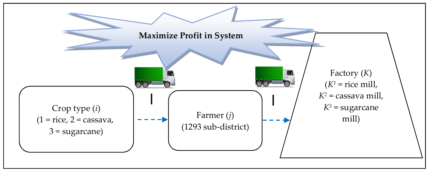
During planting of the three economic crops, each farmer was assigned to plant only one crop and each farmer was allocated a transport vehicle, considering the lowest transport costs to maximize profit. The products of each farmer were sent to the factory or purchased on-site according to the type of crop (Figure 1).

The mathematical model for economic crop planning follows.

3.1. Indices

i	stands for crop type (1 = rice, 2 = cassava, 3 = sugarcane)
j	stands for planning area/famer (j = 1, 2, …, J)
K	stands for factory (K = K1, …, Ki, when K1 = rice mill, K2 = cassava mill, K3 = sugarcane mill)

3.2. Parameters

Pij	stands for crop price i planted by farmer j (Baht/Kilogram)
C1ij	stands for cost of planning i planted by farmer j (Baht/Rai)
Bij	stands for rate of crop yield i planted by farmer j (Ton/Rai)
Aj	stands for planning area in each district (Rai)
Djk	stands for distance from planning area j to factory k (kilometer)
C2i	stands for transportation costs of each crop i (Baht/Kilometer)
CK	stands for factory purchase capacity (Ton)
C3ij	stands for cost of crop cultivation i planted by farmer j (Baht/Rai)
Vj	stands for transportation capacity (Ton)
M	stands for maximum production capacity

3.3. Decision Variables

$X_{ijk}=\{{}_{0,\mathrm{other}\mathrm{cases}}^{1,\mathrm{if}\mathrm{there}\mathrm{is}\mathrm{transportation}i\mathrm{from}\mathrm{farmer}j\mathrm{to}\mathrm{factory}k}$

$Y_{ij}=\{{}_{0,\mathrm{other}\mathrm{cases}}^{1,\mathrm{if}\mathrm{there}\mathrm{is}\mathrm{assignment}\mathrm{of}\mathrm{planting}\mathrm{crop}i\mathrm{by}\mathrm{farmer}j}$

H_ijk = Quantity factory k is given from crop i from farmer j

T¹_ij = Number of transport cycles, which must be an integer (Round)

T²_ij = Number of crop transportation i by farmer j (Round)

3.4. Objective Function

We designed and developed a mathematical model to maximize the profits for the farmers. The related factors considered were crop price, cost of each crop’s cultivation, yield rate of each crop, planning area in each district, transportation distance from planning area to factory, cost of each crop’s transportation, amount of each crop’s transportation, and cost of cultivation, which are expressed as follows:

$$\begin{gathered} \mathrm{Maximize}\mathrm{Z}={\displaystyle \sum _{i=1}^I}{\displaystyle \sum _{j=1}^J(P_{ij}-C^1{}_{ij})Y_{ij}^{}{B}_{ij}{A}_j}-{\displaystyle \sum _{i=1}^I}{\displaystyle \sum _{j=1}^J{\displaystyle \sum _{k=1}^K{X}_{ijk}^{}{D}_{jk}{C}^2{}_i{T}^2{}_{ij}}} \\ -{\displaystyle \sum _{i=1}^I}{\displaystyle \sum _{j=1}^J{Y}_{ij}}{C}^3{}_{ij} \end{gathered}$$

(1)

The objective function focused on economics to maximize profits for the farmers. Equation (1) consists of three main sequences: Sequence (1) is a function of raw materials cost, which depends on the purchase price of each crop, the cost of planting each crop, the size of planting area, and the yield rate; Sequence (2) is a function of transportation cost, which depends on the amount of raw materials, the transportation distance to factory, the cost of transportation for each crop, and the number of transportation rounds for each crop; Sequence (3) is a function of the cost of raising crops, which depends on the budget for raising each crop.

3.5. Constraints

$${\displaystyle \sum _{i=1}^I{Y}_{ij}}=1\mathrm{j}\in \mathrm{J}\forall j\in J$$

(2)

where the constraints function consists of Equation (2), which limits each farmer to planting only one crop.

$${\displaystyle \sum _{j=1}^J{Y}_{ij}^{}\ge 1}\forall i\in I$$

(3)

where Equation (3) is a limit requiring each crop to be assigned to at least one farmer.

$${{\displaystyle \sum }}_{K\in K^i}{H}_{ijk}=Y_{ij}{B}_{ij}{A}_j \forall i\in I \forall j\in J$$

(4)

where Equation (4) is a limit requiring that the amount of crop yield to be delivered to the factory must be equal to the number of crops planted by each farmer.

$$H_{ijk}\le M{X}_{ijk} \forall i\in I \forall j\in J \forall k\in K$$

(5)

where Equation (5) is a limit requiring that the amount of crop yield to be delivered to the factory must not exceed the number of crops planted by each farmer.

$${\displaystyle \sum _{k=1}^K{X}_{ijk}}\le 1\forall i\in I \forall j\in J$$

(6)

where Equation (6) is a limit requiring that a farmer can only use one transport route to the factory.

$${\displaystyle \sum _{j=1}^J{H}_{ijk}\le C_K^{}}\forall i\in I \forall K\in K^i$$

(7)

where Equation (7) is a limit requiring that the number of crops must not exceed the purchase capacity of the factory.

$$T^2{}_{ij}\ge T^1{}_{ij}\forall i\in I \forall j\in J$$

(8)

where Equation (8) limits the number of transportation rounds, which must come from the yield rate multiplied by the crop area and divided by the capacity of the transport vehicle.

$$T^1{}_{ij}=\frac{Y_{ij}{B}_{ij}{A}_j}{V_j} \forall i\in I \forall j\in J$$

(9)

where Equation (9) is a limit requiring that the number of transportation rounds be an integer (round).

$$Y_{ij}M\ge {\displaystyle \sum }_{K\in K^i}^K{X}_{ijk} \forall i\in I \forall j\in J$$

(10)

where Equation (10) is a limit requiring that the maximum yield rate delivered when a farmer is assigned crop planting must not be less than the amount of yield rate sent from the farmer to the factory.

$$Y_{ij}(bin)\forall i\in I \forall j\in J$$

(11)

where Equation (11) is a limit requiring that a farmer who plants each crop be assigned a value of 0 or 1 only; 1 for plant and 0 for others.

$$X_{ijk}(bin)\forall i\in I \forall j\in J \forall k\in K$$

(12)

where Equation (12) represents the decision variables for when farmer j transports each crop to the factory k; value 0 or 1 only.

$$H_{ijk}(gin)\forall i\in I \forall j\in J \forall k\in K$$

(13)

where Equation (13) is a limit requiring that, for the amount of crop i from farmer j to the factory k, the value is an integer.

$$T_{ij}^2(gin)\forall i\in I \forall j\in J$$

(14)

where Equation (14) is a limit requiring that the number of transportation rounds be an integer.

4. Original Differential Evolution Algorithm

We used a DE algorithm to find the solution for the crop planning problem. There were four steps involved, which are outlined below.

4.1. Initial Population

The population number (NP) is determined by a process of random sample selection from the population under a certain limit. The population group is calculated for the answer and is called the fitness value, which entails creating the preliminary answer by using the initial population. The vector is designed based on the problem statement. The proposed crop planning problem involves deciding which famers will grow which type of plant. Considering this case study, three types of plants were used: (1) rice, (2) cassava, and (3) sugarcane.

Table 1. Five vectors of the size 1 × 10.

Farmer Vector	1	2	3	4	5	6	7	8	9	10
1	0.84	0.39	0.92	0.56	0.06	0.72	0.85	0.19	0.27	0.09
2	0.71	0.45	0.40	0.63	0.78	0.07	0.49	0.81	0.71	0.30
3	0.55	0.20	0.63	0.34	0.39	0.14	0.50	0.43	0.69	0.17
4	0.80	0.75	0.49	0.76	0.74	0.55	0.11	0.34	0.65	0.51
5	0.22	0.20	0.12	0.42	0.74	0.90	0.49	0.44	0.73	0.40

shows the vector generated by the condition of having 10 farmers, 3 types of plants, and 5 populations for each iteration.

Table 1 shows the example of 5 vectors (NP = 5), with each vector having a dimension of 1 × 10 due to there being 10 farms for which to make decisions. There is one rice mill (which has a capacity of 120 tons), two sugar mills (each sugar mill has a capacity of 80 tons), and one tapioca starch mill (which has a capacity of 90 tons). Ten fields have an expected production output (in tons) if they grow different types of plants, as shown in

Table 2. Amount of product produced from each field if they grow different types of plants (ton).

-	1	2	3	4	5	6	7	8	9	10
Rice	15	20	18	8	15	13	19	21	19	15
Sugarcane	18	18	20	10	12	16	23	21	23	15
Cassava	25	16	29	9	14	20	30	19	23	16

.

The distance between each field to the factory is given in

Table 3. Distance from fields to factories. RM is rice mill, SM1 and SM2 are the two sugar mills, and TS is the tapioca starch mill.

Factory Field	RM	SM1	SM2	TS
1	279	210	148	141
2	319	186	252	332
3	107	316	199	234
4	305	323	202	272
5	285	150	158	308
6	200	245	203	179
7	189	283	173	301
8	185	122	102	326
9	291	130	141	229
10	320	125	111	141

.

4.2. Decoding Method

Table 1 and Table 2 as well as the information given above, were used to decode the continuous number to get the problem’s solution by the following steps:

(1)

Arrange the numbers in the vectors (value in position of each vector) in increasing order. For example, for Vector 1, the result of sorting is shown in

Table 4. Sorting result of Vector 1.

Farmer Vector	5	10	8	9	2	4	6	1	7	3
1	0.06	0.09	0.19	0.27	0.39	0.56	0.72	0.84	0.85	0.92

.

Taken from Table 3, it can be seen that the order of the fields is 5, 10, 8, 9, 2, 4, 6, 1, 7, and 3, which is the order according to the sorting result of the value in the position of Vector 1.

(2)

Assign the type of plant to a field and assign the field to the factory. The roulette wheel idea was used to assign the plants to the field. The probability of each plant to be selected can be determined by any idea, such as: (1) equal probability (0.333 each); (2) average productivity rate, such as rice, sugarcane, and cassava having average productivity rates of 19, 17, and 23 tons/km², with probabilities of 0.32, 0.29, and 0.39, respectively; (3) price per kilogram of the plants, for example, if the prices of rice, sugarcane, and cassava are 1000, 1200, and 900 baht per ton, the probability of each plant is 0.32, 0.39, and 0.29, respectively; (4) the ratio of factories that will take all the products. There is one rice mill, which has a capacity of 120 tons. There are two sugar mills, each of which has a capacity of 80 tons and, thus, a combined total capacity of 160 tons. There is one tapioca starch mill, which has a capacity of 90 tons. Therefore, each type of plant has a probability of 0.32, 0.43, and 0.25, respectively. During this research, we used the price per kilogram of the plants as the probability to select the plants to maximize the profits generated from the algorithm. Taken from the probability above (using price as the probability), a plant will be assigned to a field according to the value in the position of vector and that field will be assigned to the closest factory, as long as it has enough capacity. The assignment process is shown in Steps (a)–(d).

(a)

Calculate the probability of assigning the plants to the fields. Using the proposed algorithm, we applied the price of the plants to calculate this. The probabilities of assigning rice, sugarcane, and cassava were 0.32, 0.39, and 0.29, respectively, for the current example.

(b)

Calculate the cumulative probability of each type of plant. Taken from Step (2), the cumulative probabilities of rice, sugarcane, and cassava were 0.32, 0.71, and 1.0, respectively. Use the value in the vector position to decide which plants to grow. The Vector 1 position, which is Field 5, had value of 0.06. This value (0.06) falls in the rice area of the roulette wheel; therefore, Field 5 is assigned to grow rice. Then, Field 5 is assigned to the rice factory (using the information shown in Table 3). This rice factory has a 120-ton capacity and Field 5 can produce 15 tons. Thus, the rice mill has 105 tons remaining to receive rice from other fields.

(c)

Redo Step (b) until all fields are assigned to grow exactly one type of plant. This step is needed to evaluate whether a factory has enough capacity to receive the product from all fields that fall into the area of that type of plant. When the factory does not have enough capacity, the field that has a higher value in that position needs to be changed to grow other types of plants. Fields 6, 1, 7, and 3 grow cassava because the values in the Vector 1 positions for these fields were 0.72, 0.84, 0.85, and 0.92, which fall in the area of cassava, for example. However, if all addressed fields grow cassava, this will generate 104 tons of cassava. The tapioca starch mill has only a 90-ton capacity, thus the last field needs to be changed to produce other types of plants. Field 3 needs to change to produce rice in this case. The total cassava that will be produced will decrease from 104 to 75 tons and the amount of rice that will be produced in the plan will increase from 60 to 78 tons (using the information given in Table 2). The assignment of the field to the factory, in case there is more than one factory to select, can be executed by selecting to deliver the product to the factory from that field. Field 4, which grows sugarcane, needs to deliver the sugarcane to the sugar mill and there are two sugar mills, for example. Field 4 has a distance to SM1 and SM2 of 323 and 202 km, respectively (using the information given in Table 3). Therefore, Field 4 will deliver sugarcane to SM2 at a distance of 202 km.

(d)

Calculate all profit and cost terms according to the assignment obtained from Step (b).

The results of the assignment phase (Steps (a) and (b)) are shown in

Table 5. The assignment results.

Factory	Field	Plant
RM	5, 10, 8, 9, 3	Rice
SM1	2	Sugarcane
SM2	4	Sugarcane
TS	6, 1, 7	Cassava

.

4.3. Mutation Process

The mutation process was executed using Equation (15), where $V_{i,j,G}$ is the mutant vector of i position j iteration G + 1; $X_{r1,j,G}$, $X_{r2,j,G}$, and $X_{r3,j,G}$ are random target vectors 1, 2, and 3, respectively; and $F$ is the predefined scaling factor.

$$V_{i,j,G}=X_{r1,j,G}+F\left(X_{r2,j,G}-X_{r3,j,G}\right)$$

(15)

The value of the weighting factor ($F$) can range from 0 to 2 and was set to $F$ = 2.0 [65]. The value in the vector coordinate was changed by using random numbers and then entered into the mutation process (mutant vector). This conventionally is called DE/rand/1/bin.

4.4. Crossover or Recombination Process

This is a mixed species process that produces new species of better or worse results for the selection of decision variables. The result is the trial vector ($U_{i,j,G}$).

Set $CR$ = 0.8 [7,19], then enter the value exchange with Equation (16):

$$U_{i,j,G}=\{\begin{array}{ll}{V}_{i,j,G}& if Ran{d}_{i,j} \le CR\\ X_{i,j,G}& if Ran{d}_{i,j}>CR\end{array}$$

(16)

4.5. Selection Process

This is the selection process for the best answer between the target vector and the trial vector using Equation (17), which was accomplished by comparing the function value or the cost value of the trial vector with the target vector. When the function value of the trial vector was better than the target vector, it was replaced by the trial vector in the next generation.

$$X_{i,j,G+1}=\{\begin{array}{ll}{U}_{i,j,G}& if f\left(U_{i,j,G}\right)\le f\left(X_{i,j,G}\right)\\ X_{i,j,G}& otherwise\end{array}$$

(17)

Then, the answers are adjusted in each NP to determine if a better answer can be found. The answer (objective) was found from the calculation, compared against others, and the best answer was chosen from the entire population.

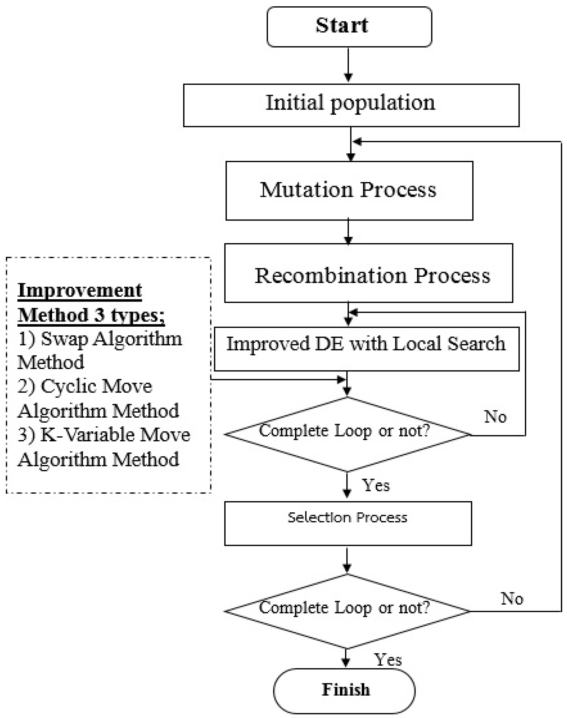
5. Improved Differential Evolution Algorithm

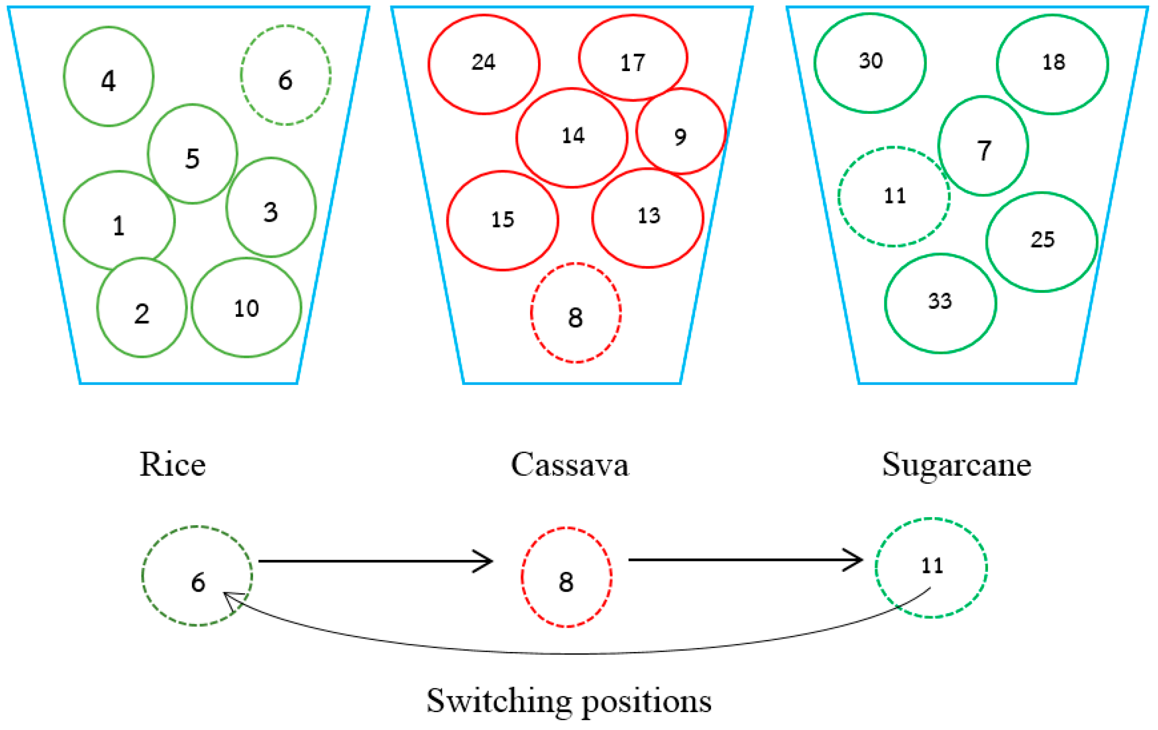
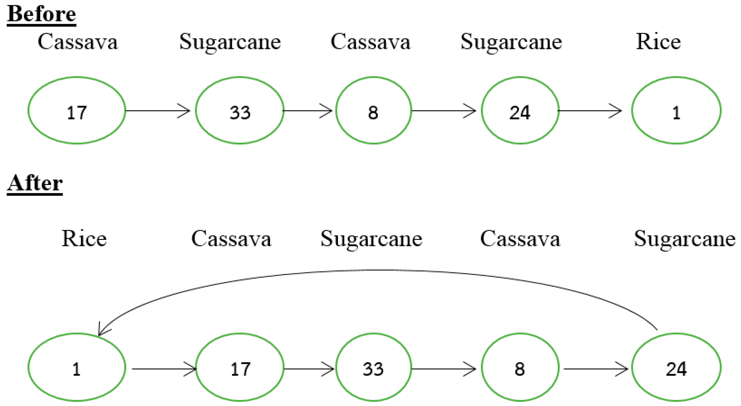
This section outlines developing and improving algorithms with DE and using Dev-C++ for testing three different-sized problems. DE is used with local search to develop the algorithm by adding a specific search step after the value exchange process in the recombination. The algorithms are developed to provide better results. There were three methods: (1) the swap algorithm, adapted from the method of Diaz and Fernandez [66]; (2) the cyclic move algorithm; and (3) the K-variable move algorithm. Figure 2 illustrates how these methods improved the steps of DE. The DE that is used in this article is conventionally called DE/rand/1/bin.

5.1. Swap Algorithm

The swap algorithm is a method used to improve a heuristic-based solution by switching pair positions between groups of members. Assuming originally that Farmer 10 is assigned to plant rice, the algorithm will switch this farmer with Farmer 24 who plants cassava to make a greater profit. Then, it will switch Farmer 8, who planted cassava, with Farmer 30, who planted sugarcane, relocating all the positions using the same process. The amount of output that the farmer sells must not exceed the capacity of the factory. The switched pairs increase the profit, as seen in Figure 3.

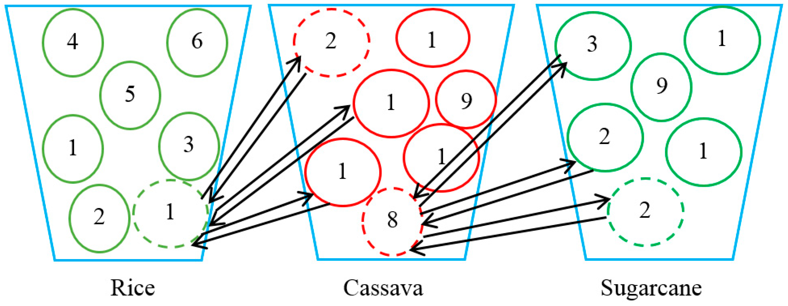
5.2. Cyclic Move Algorithm

This method selects one farmer from each group then switches each farmer in a circle. Farmer 6, who is originally assigned to plant rice, for example, is changed to cassava. Next, Farmer 8, who plants cassava, is changed to sugarcane. Additionally, Farmer 11, who plants sugarcane, is changed to rice, relocating all the positions using the same method by randomizing all rounds. Once again, the switched pairs increase the profit, as seen in Figure 4.

5.3. K-Variable Move Algorithm

To use this algorithm, K = 5 (from randomly testing all rounds), then one crop is chosen from each group, and the farmer is switched to another crop. Farmer 17, for example, is originally assigned to plant cassava and then changed to sugarcane. Next, Farmer 33, who plants sugarcane, is changed to cassava. Farmer 8, who plants cassava, is changed to sugarcane. Farmer 24, who plants sugarcane, is changed to rice. Farmer 1, who plants rice, is changed to cassava. All the positions are relocated in the same process, but the amount of output that the farmers sell must not exceed the capacity of the factory. Once again, the switched pairs increase the overall profit, as seen in Figure 5.

6. Computational Experiment and Results

The computational results are divided into two parts. First, the result of the comparison of the proposed method (DE) with the result generated by Lingo v.11 is presented to check if the proposed heuristics are reliable and trustable. Second, a simulation is used to check if the improved DE (I-DE) is better than that of the original DE to determine if the contribution of adding three local search methods to the original DE has any benefit compared to the original algorithm.

6.1. Experimental Results of Differential Evolution Algorithm (DE) Compared with Lingo V.11

We used a general DE and a developed DE to apply to and solve problems by using Dev-C++ in design algorithms, which were calculated to compare the outcome with the processing unit (Intel^® CoreTM i5-2410M 2.3 GHz and 4 GB memory). DE ran five replicates and the best solution among all five runs was the solution represented in

Table 6. Experimental results of the Differential Evolution (DE) algorithm compared with Lingo v.11.

Problem Group	Farmer or Subdistrict	Rice	Cassava	Sugarcane	Methods
		Number of Factories	Number of Factories	Number of Factories	Lingo		Differential Evolution Algorithm (DE)
-	-	-	-	-	Solution (Baht)	Time (s)	Solution	Time (s)
1 (Small Size)	5	3	3	4	153,040	00:00:02	153,040	00:00:01
	10	3	3	4	538,909	00:00:05	538,909	00:00:03
	15	3	3	4	704,463	00:00:27	704,463	00:00:05
	20	7	7	5	1.1175 × 106	00:00:46	1.1175 × 106	00:00:14
2 (Medium size)	40	16	30	5	2.4585 × 106	00:03:39	2.4585 × 106	00:00:23
	60	30	50	5	3.73617 × 106	00:06:50	3.73617 × 106	00:01:38
	70	35	55	3	4.31865 × 106	00:10:25	4.31865 × 106	00:03:37
3 (Large Size)	80	45	60	5	4.3341 × 106	250 h *	4.45924 × 106	00:02:13
	80	50	70	7	4.3378 × 106	250 h *	4.75384 × 106	00:03:26
	80	55	70	10	4.3467 × 106	250 h *	4.68498 × 106	00:03:69
	100	60	70	10	4.3593 × 106	250 h *	4.54516 × 106	00:10:16
	100	60	80	10	4.4355 × 106	250 h *	4.61473 × 106	00:13:10
	100	60	80	10	4.4355 × 106	250 h *	4.51473 × 106	00:13:10
	500	70	85	13	5.13148 × 106	250 h	5.18148 × 106	00:16:34
Case study	1293	95	98	19	1.39234 × 107	250 h *	1.41761 × 107	00:21:82

Remarks: * Best solution generated in 250 h.

. The problem instances were categorized into three groups: (1) small problem group, 5–20 farmers; (2) medium problem group, 40–70 farmers; and (3) large problem group, 80–500 farmers. Four test instances were randomly generated for the small-size instances, whereas three test instances were generated for medium- and large-size test instances. One real case study was used in the simulation test. The authors had 11 test instances in total. The stopping criterion for Lingo was set to when it found the optimal solution, with a maximum duration of 250 h. The stopping criterion of DE was the number of iterations, with a threshold of 500 iterations. Set NP = 50, F = 2.0, and CR = 0.8 [7,19]. The results of DE compared with Lingo v.11 are shown in Table 6.

Looking at the results in Table 6, it can be seen that the small- and medium-sized test instances of DE can find the same solution as Lingo v.11, using lower computational time. Regarding the large-size instances (including the case study), DE generated a better solution than that of Lingo v.11, which ran for 250 h, whereas DE ran for a maximum of 21.82 min to obtain the result. DE used less computational time in all test instances than Lingo v.11. The Wilcoxon signed-rank test was applied using a 95% confidence interval to compare the results of DE and Lingo v.11, which provided significant evidence to conclude that the results generated by Lingo v.11 and DE were different (p-value = 0.004 and α = 0.05). Therefore, we concluded that DE can find a better solution than Lingo v.11 when Lingo v.11 has a computational limit time set to 250 h (p-value = 0.043 and α = 0.05).

6.2. Experimental Results of DE Compared with Modified DE

The authors had three improved DE algorithms (I-DE), which were I-DE-SW (DE + swap algorithm), I-DE-CY (DE + cyclic move algorithm), and I-DE-KV (DE + K-variable move algorithm). The stopping criterion used in this session was a 2 h simulation time. Five simulation runs were performed and the best solution among all runs is shown in

Table 7. Overall profitability for the general DE and Improved DE (I-DE) methods with equal duration.

Problem Size	N	Solution (Profit: Baht)
	(A-B-C)	DE	I-DE-SW	I-DE-CY	I-DE-KV
Small size	5 (3-3-4)	153,040	208,933	153,040	208,933
	10 (3-3-4)	538,909	565,109	554,117	565,109
	15 (3-3-4)	704,463	704,463	704,219	704,219
	20 (7-7-5)	1.1175 × 106	1.10857 × 106	1.11875 × 106	1.11877 × 106
Medium size	40 (16-30-5)	2.4585 × 106	2.4585 × 106	2.4585 × 106	2.4585 × 106
	60 (30-50-5)	3.73617 × 106	3.73617 × 106	3.73617 × 106	3.73711 × 106
	70 (35-55-3)	4.31865 × 106	4.31865 × 106	4.31865 × 106	4.31865 × 106
Large size	80 (45-60-5)	4.55924 × 106	4.55924 × 106	4.55924 × 106	4.56032 × 106
	80 (50-70-7)	4.47249 × 106	4.65214 × 106	4.69214 × 106	4.71241 ×106
	80 (55-70-10)	4.78129 × 106	4.79241 × 106	4.79201 × 106	4.84542 × 106
	100 (60-70-10)	4.55681 × 106	4.60241 × 106	4.61042 × 106	4.72124 × 106
	100 (60-80-10)	4.64981 × 106	4.76292 × 106	4.75124 × 106	4.78419 × 106
	100 (60-80-10)	4.65924 × 106	4.71105 × 106	4.70924 × 106	4.72149 × 106
	500 (70-85-13)	5.23148 × 106	5.36866 × 106	5.3548 × 106	5.37866 × 106
Case study	1293 (95-98-19)	1.427614 × 107	1.457129 × 107	14.32278 × 106	14.59643 × 106

Note: N stands for Farmers, A stands for rice mill, B stands for cassava mill, and C stands for sugarcane mill.

.

Table 7 shows the experiment used to compare the efficiency of the original DE with the I-DEs using the same duration (two hours). I-DE-KV provided the most effective answer and most comprehensive range of answers compared with the other methods, especially for the large-size problems and the case study for 1293 farmers. The best answer for the case study generated by I-DE-KV was 14,596,430 baht per crop cycle. I-DE-KV could also show the factory location and areas for economic crop planning.

The pair t-test has been executed using significant level α = 0.05 and the result is shown in

Table 8. Pair t-test results (sign (p-value)).

Method	I-DE-SW	I-DE-CY	I-DE-KV
DE	≤(0.02 *)	≤(0.012 *)	≤(0.009 *)
I-DE-SW	-	=(0.403)	≤(0.038 *)
I-DE-CY	-	-	≤(0.036 *)

Note: * means significantly different.

. The statistical test was performed only with the large instances. Considering the small and medium instances, it can be seen that DE and the proposed algorithm were not different (all results are the same).

Viewing the statistical test shown in Table 8, I-DE-SW and I-DE-CY were significantly different to I-DE-KV. Thus, the K-variable move improved the solution quality of the DE algorithm. Additionally, I-DE-SW and I-DE-CY performance was not significantly different, which can be interpreted that when a local search in DE is added, it can improve the efficiency of DE (all proposed methods were significantly different from DE). This might be changed if a local search does not perform differently, especially when the neighborhood size is unaltered.

The last experiment tested I-DE-KV (computational time is set to two hours), which was the best proposed algorithm with the upper bound (maximization problem), and the best solution generated from Lingo v.11 within 200, 250, 300, 350, and 400 h. The result is shown in

Table 9. Result of Lingo v.11 (Upper Bound and Best Objective) and I-DE algorithm using K-variable move (I-DE-KV).

Time	Method	200 h	250 h	300 h	350 h	400 h
Instance
80 (45-60-5)	Upper Bound	4.58894 × 106	4.58894 × 106	4.58894 × 106	4.57591 × 106	4.57591 × 106
	Best Objective	4.55145 × 106	4.55145 × 106	4.55981 × 106	4.55981 × 106	4.55981 × 106
	I-DE-KV	4.56032 × 106
80 (50-70-7)	Upper Bound	4.80512 × 106	4.80512 × 106	4.78214 × 106	4.78214 × 106	4.76542 × 106
	Best Objective	4.56821 × 106	4.56995 × 106	4.58912 × 106	4.60156 × 106	4.60156 × 106
	I-DE-KV	4.71241 × 106
80 (55-70-10)	Upper Bound	4.90124 × 106	4.90259 × 106	4.899128 × 106	4.899128 × 106	4.899128 × 106
	Best Objective	4.71249 × 106	4.71249 × 106	4.71249 × 106	4.71249 × 106	4.71249 × 106
	I-DE-KV	4.84542 × 106
100 (60-70-10)	Upper Bound	4.98241 × 106	4.85215 × 106	4.79242 × 106	4.79242 × 106	4.79242 × 106
	Best Objective	4.61983 × 106	4.62488 × 106	4.62488 × 106	4.62488 × 106	4.63245 × 106
	I-DE-KV	4.72124 × 106
100 (60-80-10)	Upper Bound	4.88812 × 106	4.88812 × 106	4.85289 × 106	4.85289 × 106	4.81457 × 106
	Best Objective	4.62388 × 106	4.62388 × 106	4.62388 × 106	4.64514 × 106	4.64514× 106
	I-DE-KV	4.73419 × 106
100 (60-80-10)	Upper Bound	4.8190 × 106	4.8190 × 106	4.8024 × 106	4.8024 × 106	4.79842 × 106
	Best Objective	4.6786 × 106	4.69782 × 106	4.70113 × 106	4.70113 × 106	4.70113 × 106
	I-DE-KV	4.71105 × 106
500 (70-85-13)	Upper Bound	5.46991 × 106	5.46991 × 106	5.46892 × 106	5.46892 × 106	5.44412 × 106
	Best Objective	5.34917 × 106	5.35178 × 106	5.35178 × 106	5.35980 × 106	5.35991 × 106
	I-DE-KV	5.37866 × 106
1293 (95-98-19)	Upper Bound	14.7919 × 106	14.7919 × 106	14.7919 × 106	14.7814 × 106	14.7814 × 106
	Best Objective	14.56891 × 106	14.56891 × 106	14.57129 × 106	14.57643 × 106	14.57610 × 106
	I-DE-KV	14.59643 × 106

. The simulation considers only the large problem and the case study.

Concerning Table 9, “Upper Bound” is the upper bound found by Lingo v.11 within the predefined computational times (200, 250, 300, 350, and 400 h) and “Best Objective” is the best objective found by Lingo v.11 within the predefined computational times. The I-DE-KV result is the outcome of the proposed heuristics using two hours as the computational time. Taken from Table 9, it can be simplified into $\%diff$, which can be calculated from Equation (18):

$$\%diff.=\frac{Result from Candidate Method-Result from \mathrm{I}-\mathrm{DE}-\mathrm{KV}}{Result from \mathrm{I}-\mathrm{DE}-\mathrm{KV}}\times 100\%$$

(18)

Table 10. $\%diff$ of the candidate method and I-DE-KV.

Time	Method	200 h	250 h	300 h	350 h	400 h
Instance
80 (45-60-5)	Upper Bound	0.628	0.628	0.628	0.342	0.342
	Best Objective	–0.195	−0.195	−0.011	−0.011	−0.011
80 (50-70-7)	Upper Bound	1.967	1.967	1.480	1.480	1.125
	Best Objective	−3.060	−3.023	−2.616	−2.352	−2.352
80 (55-70-10)	Upper Bound	1.152	1.180	1.108	1.108	1.108
	Best Objective	−2.743	−2.743	−2.743	−2.743	−2.743
100 (60-70-10)	Upper Bound	5.532	2.773	1.508	1.508	1.508
	Best Objective	−2.148	−2.041	−2.041	−2.041	−1.881
100 (60-80-10)	Upper Bound	3.251	3.251	2.507	2.507	1.698
	Best Objective	−2.330	−2.330	−2.330	−1.881	−1.881
100 (60-80-10)	Upper Bound	2.291	2.291	1.939	1.939	1.855
	Best Objective	−0.689	−0.281	−0.211	−0.211	−0.211
500 (70-85-13)	Upper Bound	1.697	1.697	1.678	1.678	1.217
	Best Objective	−0.548	−0.500	−0.500	−0.351	−0.349
1293 (95-98-19)	Upper Bound	1.339	1.339	1.339	1.267	1.267
	Best Objective	−0.189	−0.189	−0.172	−0.137	−0.139
Average	Upper Bound	2.232	1.891	1.523	1.479	1.265
	Best Objective	−1.488	−1.413	−1.328	−1.216	−1.196

shows the $\%diff$ of the Upper Bound and the Best Objective found by Lingo v.11 using different computational times.

Table 10 shows that the Upper Bound has all positive $\%diff$ values, and Best Objective has negative $\%diff$ values. This means that Upper Bound generates more profit to the system than I-DE-KV, but Best Objective has lower profits than I-DE-KV. Upper Bound can be a feasible or an infeasible solution. Therefore, it generates a better solution than the DE algorithm. The Best Objective is a feasible solution and it is the best solution found during the simulation. Taken from this, we concluded that the DE algorithm can find a better solution than Lingo v.11, and Lingo v.11 uses a computational time of 200–400 h and DE runs for only two hours. The average $\%diff$ of I-DE-KV and Upper Bound generated by Lingo v.11, when using 200, 250, 300, 350, and 400 h of computational time were 2.232, 1.891, 1.523, 1.479, and 1.265%, respectively. The $\%diff$ of Best Objective and I-DE-KV ranged from −1.488 to −1.196%. Further, I-DE-KV had a gap of only 0.342–5.532% from the Upper Bound, from which we concluded that it is an effective algorithm. The pair t-test was used to see if I-DE-KV performed differently than Upper Bound and Best Objective found by Lingo v.11. The result is shown in

Table 11. Statistical test of I-DE-KV and Upper Bound and Best Objective found by Lingo v.11.

Method		Best Objective	I-DE-KV
Lingo	Upper Bound	≥(0.001 *)	≥(0.003 *)
	Best Objective	-	≤(0.003 *)

Note: * means significantly different.

.

Looking at Table 11, it can be seen that Upper Bound has a significantly higher benefit than Best Objective and I-DE-KV. Upper Bound normally contains an infeasible solution. The Best Objective has significantly lower benefit than I-DE-KV with a 95% confidence interval.

7. Conclusions

This study aimed to solve the economic crop planning allotment problem for farmers in eight provinces in the lower northeast region of Thailand by improving mathematical models and algorithms and by considering the economic value of maximizing profits for the farmers. The study focused on three economic crops—rice, cassava, and sugarcane—and used a DE algorithm to solve the problems to maximize profits for the farmers. The outcomes and running times of the DE algorithms were compared with Lingo v.11. When comparing the performance of all algorithms using DE in small-size problem simulations, DE had the best performance and enhanced the chance of finding a better outcome.

Three improved DE algorithms were proposed in this article: I-DE-SW, I-DE-CY, and I-DE-KV. Viewing the computational results, I-DE-KV generated the best method compared to all other methods proposed, including the original DE algorithm. All the I-DE algorithms found better solutions than the original DE. We concluded that a DE algorithm that includes local search can improve the efficiency of the original version. The swap algorithm limited the number of entities involved to two, the cyclic move algorithm had three entities involved, and the K-variable move algorithm can have two, three, four, or more depending on the random value of K. This attribute makes the K-variable move algorithm freer and more flexible, thus enabling it to generate the best solution among all proposed heuristics while using the same computational time.

Comparing I-DE-KV with Upper Bound, the proposed method resulted in a 1.265–2.232% difference from the Upper Bound. I-DE-KV found a 1.196–1.488% higher profit than that of the best solution found by Lingo v.11 using 400 h computational time, whereas DE only required two hours.

Therefore, the proposed heuristic is an effective algorithm for finding a good solution to the crop planning problem. It uses more than 200 times less computational time than that of Lingo v.11 while generating a better solution. Future work should focus on using different kinds of attractiveness to assign the plants to the fields.

The advantage of the proposed heuristic is that it is fast and can find a better solution in comparison to the results generated from Lingo v.11 when the problem size is large. The computational times when the problem size is small are not much different from that of Lingo v.11. Due to DE working on the random environment using a guided search, sometimes the guided search leads to a bad search area, which can result in local optimization and generate a worse solution than that of Lingo v.11—the optimization tool which always finds the lowest cost. The decision-maker must clarify the problem size first before making the decision to use optimization tools or metaheuristics to obtain the optimal solution.

References

1. Agricultural Information Office. Agricultural Information; Agricultural Economics, Ministry of Agriculture and Cooperatives: Bangkok, Thailand, 2016. [Google Scholar]
2. Thongdee, T.; Pitakaso, R. Differential Evolution Algorithms Solving a Multi-Objective, Source and Stage Location-Allocation Problem. Ind. Eng. Manag. Syst. 2015, 14, 11–21. [Google Scholar] [CrossRef] [Green Version]
3. Sethanan, K.; Pitakaso, R. Improved differential evolution algorithms for solving generalized assignment problem. Expert Syst. Appl. 2016, 45, 450–459. [Google Scholar] [CrossRef]
4. Wang, G.; Tan, Y. Improving Metaheuristic Algorithms with Information Feedback Models. IEEE Trans. Cybern. 2017, 99, 1–14. [Google Scholar] [CrossRef] [PubMed]
5. Wang, G.; Guo, L.; Gandomi, A.H.; Hao, G.; Wang, H. Chaotic Krill Herd algorithm. Inf. Sci. 2014, 274, 17–34. [Google Scholar] [CrossRef]
6. Wang, G.; Gandomi, A.H.; Alavi, A.H. An effective krill herd algorithm with migration operator in biogeography-based optimization. Appl. Math. Model. 2014, 38, 2454–2462. [Google Scholar] [CrossRef]
7. Cui, Z.; Sun, B.; Wang, G.; Xue, Y.; Chen, J. A novel oriented cuckoo search algorithm to improve DV-Hop performance for cyber-physical systems. J. Parallel Distrib. Comput. 2016, 103. [Google Scholar] [CrossRef]
8. Wang, G.; Alavi, A.H.; Zhao, X.J.; Hai, C.C. Hybridizing harmony search algorithm with cuckoo search for global numerical optimization. Soft Comput. 2016, 20, 273–285. [Google Scholar] [CrossRef]
9. Feng, Y.; Wang, G. Binary Moth Search Algorithm for Discounted {0–1} Knapsack Problem. IEEE Access 2018. [Google Scholar] [CrossRef]
10. Wang, G.; Deb, S.; Cui, Z. Monarch Butterfly Optimization. Neural Comput. Appl. 2015. [Google Scholar] [CrossRef]
11. Wang, G.; Guo, L.; Gandomi, A.H.; Cao, L.; Alavi, A.H.; Duan, H.; Li, J. Lévy-Flight Krill Herd Algorithm. Math. Probl. Eng. 2013. [Google Scholar] [CrossRef]
12. Wang, G.; Guo, L.; Duan, H.; Wang, H.; Liu, L.; Shao, M. Hybridizing Harmony Search with Biogeography Based Optimization for Global Numerical Optimization. J. Comput. Theor. Nanosci. 2013, 10, 2312–2322. [Google Scholar] [CrossRef]
13. Wei, Z.J.; Wang, G. Image Matching Using a Bat Algorithm with Mutation. Appl. Mech. Mater. 2012, 203, 88–93. [Google Scholar] [CrossRef]
14. Wang, G.; Coelho, L.; Gao, X.Z.; Deb, S. A new metaheuristic optimisation algorithm motivated by elephant herding behavior. Int. J. Bio-Inspired Comput. 2016, 8. [Google Scholar] [CrossRef]
15. Wang, G.; Deb, S.; Coelho, L.D.S. Earthworm optimization algorithm: A bio-inspired metaheuristic algorithm for global optimization problems. Int. J. Bio-Inspired Comput. 2018, 12, 1–12. [Google Scholar] [CrossRef]
16. Wang, G.; Guo, L.; Wang, H.; Duan, H.; Liu, L.; Li, J. Incorporating mutation scheme into krill herd algorithm for global numerical optimization. Neural Comput. Appl. 2014, 24, 853–871. [Google Scholar] [CrossRef]
17. Wang, G.; Gandomi, A.H.; Alavi, A.H. Stud krill herd algorithm. Neurocomputing 2014, 128, 363–370. [Google Scholar] [CrossRef]
18. Wang, G.; Gandomi, A.H.; Yang, X.; Alavi, A.H. A new hybrid method based on krill herd and cuckoo search for global optimisation tasks. Int. J. Bio-Inspired Comput. 2016, 8, 286–299. [Google Scholar] [CrossRef]
19. Wang, H.; Yi, J.H. An improved optimization method based on krill herd and artificial bee colony with information exchange. Memet. Comput. 2017, 10, 177–198. [Google Scholar] [CrossRef]
20. Wang, G.; Gandomi, A.H.; Alavi, A.H.; Deb, S. A hybrid method based on krill herd and quantum-behaved particle swarm optimization. Neural Comput. Appl. 2016, 27, 989–1006. [Google Scholar] [CrossRef]
21. Wang, G.; Guo, L.; Gandomi, A.H.; Alavi, A.H.; Duan, H. Simulated Annealing-Based Krill Herd Algorithm for Global Optimization. Abstr. Appl. Anal. 2013. [Google Scholar] [CrossRef]
22. Guo, L.; Wang, G.; Gandomi, A.H.; Alavi, A.H.; Duan, H. A new improved krill herd algorithm for global numerical optimization. Neurocomputing 2014, 138, 392–402. [Google Scholar] [CrossRef]
23. Wang, G.; Gandomi, A.H.; Alavi, A.H. Study of Lagrangian and Evolutionary Parameters in Krill Herd Algorithm. In Adaptation and Hybridization in Computational Intelligence. Adaptation, Learning, and Optimization; Fister, I., Fister, I., Jr., Eds.; Springer: Cham, Switzerland, 2015. [Google Scholar]
24. Wang, G.; Gandomi, A.H.; Alavi, A.H.; Deb, S. A Multi-Stage Krill Herd Algorithm for Global Numerical Optimization. Int. J. Artif. Intell. Tools 2016, 25. [Google Scholar] [CrossRef]
25. Wang, G.; Deb, S.; Gandomi, A.H.; Alavi, A.H.A. Opposition-based krill herd algorithm with Cauchy mutation and position clamping. Neurocomputing 2016, 177, 147–157. [Google Scholar] [CrossRef]
26. Wang, G.; Gandomi, A.H.; Alavi, A.H.; Gong, D. A comprehensive review of krill herd algorithm: Variants, hybrids and applications. Artif. Intell. Rev. 2017. [Google Scholar] [CrossRef]
27. Rizk, M.; Rizk, A.; Ragab, A.; El-Sehiemy, R.A.; Wang, G. A novel parallel hurricane optimization algorithm for secure emission/economic load dispatch solution. Appl. Soft Comput. 2018, 63, 206–222. [Google Scholar] [CrossRef]
28. Wang, G.; Gandomi, A.H.; Alavi, A.H.; Dong, Y. A Hybrid Meta-Heuristic Method Based on Firefly Algorithm and Krill Herd. In Handbook of Research on Advanced Computational Techniques for Simulation-Based Engineering; IGI: Hershey, PA, USA, 2016; pp. 521–540. [Google Scholar]
29. Wang, G. Moth search algorithm: A bio-inspired metaheuristic algorithm for global optimization problems. Memet. Comput. 2018, 10, 151–164. [Google Scholar] [CrossRef]
30. Feng, Y.; Wang, G.; Deb, S.; Lu, M.; Zhao, X. Solving 0–1 knapsack problem by a novel binary monarch butterfly optimization. Neural Comput. Appl. 2017, 28, 1619–1634. [Google Scholar] [CrossRef]
31. Feng, Y. Solving 0–1 knapsack problems by chaotic monarch butterfly optimization algorithm with Gaussian mutation. Memet. Comput. 2016. [Google Scholar] [CrossRef]
32. Wang, G.; Deb, S.; Zhao, X.; Cui, Z. A new monarch butterfly optimization with an improved crossover operator. Oper. Res. 2016. [Google Scholar] [CrossRef]
33. Wu, G. Across neighborhood search for numerical optimization. Inf. Sci. 2016, 329, 597–618. [Google Scholar] [CrossRef] [Green Version]
34. Wang, G.; Gandomi, A.H.; Alavi, A.H. A chaotic particle-swarm krill herd algorithm for global numerical optimization. Kybernetes 2013, 42, 962–978. [Google Scholar] [CrossRef]
35. Wang, G.; Deb, S.; Gandomi, A.H.; Zhang, Z.; Alavi, A.H. Haotic cuckoo search. Soft Comput. Fusion Found. Methodol. Appl. 2016, 20, 3349–3362. [Google Scholar]
36. Yi, J.; Wang, J.; Wang, G. Improved probabilistic neural networks with self-adaptive strategies for transformer fault diagnosis problem. Adv. Mech. Eng. 2016, 8. [Google Scholar] [CrossRef] [Green Version]
37. Storn, R.; Price, K.V. Differential evolution: A simple and efficient adaptive scheme for global optimization over continuous spaces. J. Glob. Optim. 1995, 11, 341–359. [Google Scholar] [CrossRef]
38. Erbao, C.; Lai, M. A Hybrid differential evolution algorithm to vehicle routing problem with fuzzy demands. J. Comput. Appl. Math. 2009, 231, 302–310. [Google Scholar] [CrossRef]
39. Dechampai, D.; Tanwannichkul, L.; Sethanan, K.; Pitakaso, R. A differential evolution algorithm for the capacitated VRP with Flexibility for mixing pickup and delivery services and the maximum duration route in poultry industry. J. Intell. Manuf. 2017, 28, 1357–1376. [Google Scholar] [CrossRef]
40. Sethanan, K.; Pitakaso, R. Differential evolution algorithms for scheduling raw milk transportation. Comput. Electron. Agric. 2016, 121, 245–259. [Google Scholar] [CrossRef]
41. Das, S.; Suganthan, P.N. Differential Evolution: A Survey of the State-of-the-Art. IEEE Trans. Evol. Comput. 2011, 15, 4–31. [Google Scholar] [CrossRef]
42. Glen, J.J. Mathematical models in farm planning: A survey. Oper. Res. 1987, 35, 641–666. [Google Scholar] [CrossRef] [Green Version]
43. Itoh, T.; Ishii, H.; Nanseki, T. A model of crop planning under uncertainty in agricultural management. Int. J. Prod. Econ. 2003, 81, 555–558. [Google Scholar] [CrossRef]
44. Sarker, R.A.; Talukdar, S.; Haque, A. Determination of optimum crop mix for crop cultivation in Bangladesh. Appl. Math. Model. 1997, 21, 621–632. [Google Scholar] [CrossRef]
45. Santosa, B.; Sunarto, A.; Rahman, A. Using Differential Evolution Method to Solve Crew Rostering Problem. Appl. Math. 2010, 1, 316–325. [Google Scholar] [CrossRef]
46. Adeyemo, J.; Otieno, F. Differential evolution algorithm for solving multi-objective crop planning model. Agric. Water Manag. 2010, 97, 848–856. [Google Scholar] [CrossRef]
47. Mallipeddi, R.; Suganthan, P.N.; Pan, Q.K.; Tasgetiren, M.F. Differential evolution algorithm with ensemble of parameters and mutation strategies. Appl. Soft Comput. 2010, 11, 1679–1696. [Google Scholar] [CrossRef]
48. Adekanmbi, O.A.; Olugbara, O.O.; Adeyemo, J. A Comparative Study of State-of-the-Art Evolutionary Multi-objective Algorithms for Optimal Crop-mix planning. Int. J. Agric. Sci. Technol. 2014, 2, 8–16. [Google Scholar] [CrossRef]
49. Adeyemo, J.; Bux, F.; Otieno, F. Differential evolution algorithm for crop planning: Single and multi-objective optimization model. Int. J. Phys. Sci. 2010, 5, 1592–1599. [Google Scholar]
50. Pant, M.; Radha, T.; Rani, D.; Abraham, A.; Srivastava, D.K. Estimation Using Differential Evolution for Optimal Crop Plan. In Proceedings of the HAIS 2008 International Conference on Hybrid Artificial Intelligence Systems, Oviedo, Spain, 20–22 June 2008; pp. 289–297. [Google Scholar]
51. Yi, H.; Duan, Q.; Liao, T.W. Three improved hybrid metaheuristic algorithms for engineering design optimization. Appl. Soft Comput. 2013, 13, 2433–2444. [Google Scholar] [CrossRef]
52. Wang, G.; Cheng, H.; Chu, E.; Mirjalili, S. Three-dimensional path planning for UCAV using an improved bat algorithm. Aerosp. Sci. Technol. 2016, 49, 231–238. [Google Scholar] [CrossRef]
53. Wang, G.; Gandomi, A.H.; Alavi, A.H.; Hao, G. Hybrid krill herd algorithm with differential evolution for global numerical optimization. Neural Comput. Appl. 2014, 25, 297–308. [Google Scholar] [CrossRef]
54. Wang, G.; Gandomi, A.H.; Yang, Z.; Alavi, A.H. A novel improved accelerated particle swarm optimization algorithm for global numerical optimization. Eng. Comput. 2014, 31, 1198–1220. [Google Scholar] [CrossRef]
55. Wu, G.; Shen, X.; Li, H.; Chen, H.; Lin, A.; Suganthan, P.N. Ensemble of differential evolution variants. Inf. Sci. 2018, 423, 172–186. [Google Scholar] [CrossRef]
56. Wu, G.; Pedrycz, W.; Suganthan, P.N.; Lie, H. Using variable reduction strategy to accelerate evolutionary optimization. Appl. Soft Comput. 2017, 61, 283–293. [Google Scholar] [CrossRef]
57. Wang, R.; Purshouse, R.C.; Fleming, P.J. Preference-Inspired Coevolutionary Algorithms for Many-Objective Optimization. IEEE Trans. Evol. Comput. 2013, 17, 474–494. [Google Scholar] [CrossRef]
58. Wang, R.; Zhang, O.; Zhang, T. Decomposition-Based Algorithms Using Pareto Adaptive Scalarizing Methods. IEEE Trans. Evol. Comput. 2016, 20, 821–837. [Google Scholar] [CrossRef]
59. Wu, G.; Pedrycz, W.; Li, H.; Ma, M.; Liu, J. Coordinated Planning of Heterogeneous Earth Observation Resources. IEEE Trans. Syst. Man Cybern. Syst. 2016, 46, 109–125. [Google Scholar] [CrossRef]
60. Wang, G.; Guo, L.; Duan, H.; Wang, H. A New Improved Firefly Algorithm for Global Numerical Optimization. J. Comput. Theor. Nanosci. 2014, 11, 477–485. [Google Scholar] [CrossRef]
61. Wang, G.; Cai, X.; Cui, Z.; Min, G.; Chen, J. High Performance Computing for Cyber Physical Social Systems by Using Evolutionary Multi-Objective Optimization Algorithm. IEEE Trans. Emerg. Top. Comput. 2017. [Google Scholar] [CrossRef]
62. Ke, L.; Gong, D.W.; Meng, F.L.; Chen, H.H.; Wang, G. Gesture segmentation based on a two-phase estimation of distribution algorithm. Inf. Sci. 2017. [Google Scholar] [CrossRef]
63. Rizk, R.M.; El-Sehiemy, R.A.; Deb, S.; Wang, G. A novel fruit fly framework for multi-objective shape design of tubular linear synchronous motor. J. Supercomput. 2017, 73, 1235–1256. [Google Scholar] [CrossRef]
64. Wang, R.; Zhou, Z.; Ishibuchi, H.; Liao, T.; Zhang, T. Localized Weighted Sum Method for Many-Objective Optimization. IEEE Trans. Evol. Comput. 2018, 22, 3–18. [Google Scholar] [CrossRef]
65. Qin, A.K.; Huang, V.L.; Suganthan, P.N. Differential evolution algorithm with strategy adaptation for global numerical optimization. IEEE Trans. Evolut. Comput. 2009, 13, 398–417. [Google Scholar] [CrossRef]
66. Diaz, J.A.; Fernandez, E. A Tabu search heuristic for the generalized assignment problem. Eur. J. Oper. Res. 2001, 132, 22–38. [Google Scholar] [CrossRef]
Figure 1. Model of transport of economic crops from the farmer to the factory.
Mca 23 00040 g001
Figure 2. Steps using improved Differential Evolution (DE) algorithm with three local search methods.
Mca 23 00040 g002
Figure 3. An example of developing an answer by the swap algorithm.
Mca 23 00040 g003
Figure 4. An example of developing an answer by the cyclic move algorithm.
Mca 23 00040 g004
Figure 5. An example of developing an answer by the K-variable move algorithm.
Mca 23 00040 g005