Cellular Automata and Artificial Brain Dynamics

Abstract

Brain dynamics, neuron activity, information transfer in brains, etc., are a vast field where a large number of questions remain unsolved. Nowadays, computer simulation is playing a key role in the study of such an immense variety of problems. In this work, we explored the possibility of studying brain dynamics using cellular automata, more precisely the famous Game of Life (GoL). The model has some important features (i.e., pseudo-criticality, 1/f noise, universal computing), which represent good reasons for its use in brain dynamics modelling. We have also considered that the model maintains sufficient flexibility. For instance, the timestep is arbitrary, as are the spatial dimensions. As first steps in our study, we used the GoL to simulate the evolution of several neurons (i.e., a statistically significant set, typically a million neurons) and their interactions with the surrounding ones, as well as signal transfer in some simple scenarios. The way that signals (or life) propagate across the grid was described, along with a discussion on how this model could be compared with brain dynamics. Further work and variations of the model were also examined.

1. Introduction

The question “Can cellular automata model brain dynamics?” or in our case “Can the Game of Life model brain dynamics?” is hard to answer for, at least, three reasons. First, despite decades of efforts to understand the Game of Life (GoL hereafter), several questions remain unanswered. Second, although brain dynamics is an exponentially growing field in neuroscience, several questions remain under strong debate. Third, it is still not known which characteristics are fundamental in brain dynamics and which characteristics are derived from (or are dependent upon) a particular biological realization. Hence, the goal of this study was fairly ambitious and only some possible ideas and paths to follow were presented.

Cellular automata (CA) have been studied since the early 1950’s [1,2,3] in connection with many different problems, such as predator–prey, [4,5] chemistry, [6] dendritic growth [7], and many more. For instance, Reference [8] provides a review of the biological applications. Different CA have been used in several problems related to neuroscience [9,10,11,12,13]. Amongst the various CA, the GoL was chosen because it presents several characteristics that are, in our opinion, good reasons to associate brain dynamics with the evolution of life as modelled using the GoL. It is an established idea in science, particularly in chaos theory and complex systems, that very simple rules can often generate great complexity [14], and probably nothing in nature is more complex than the human brain.

The brain was included amongst the abundance of physical and biological systems that exhibit different levels of criticality, as described in References [15,16,17] and the references therein. To function optimally, neuronal networks were considered to operate close to a non-equilibrium critical point [18]. However, recent works provide evidence that the human brain operates not in a critical state, but rather it keeps a distance to criticality [19,20,21], despite the computational advantages of criticality [22]. Therefore, it appears that maximization of information processing is not the only goal function of the brain. According to these results, the brain only tunes itself closer to criticality when it is necessary for information processing. Otherwise, the brain maintains a safety margin, losing processing capacity, but avoiding instabilities (e.g., an epileptic crisis) [19,20,21]. This hypothesis, however, is still controversial [23,24,25,26].

GoL was originally supposed to present self-organized criticality (SOC). Power-law decay of several statistical quantities was interpreted as evidence of SOC [27]. For example, the distribution D(T) of time steps required for the lattice to return to stability following a random single-site perturbation is characterized by D(T) ~ T^−1.6 [27]. More recently, Hemmingsson [28] suggested that the GoL does not converge to a SOC state, but it is in fact subcritical with a long length scale. Additional evidence has also been put forward by Nordfalk et al [29], wherein this capacity of the GoL model suggests a connection to brain dynamics.

A second point is that the GoL presents a 1/f noise [30], a feature that is believed to be present in brain dynamics [31,32] in electro- and magneto-encephalogram spectra (EEG and MEG) [33], and in human cognition as well [34]. Results suggest that there is a relationship between computational universality and 1/f noise in cellular automata [30]. However, discussion continues regarding whether or not 1/f noise is evidence of SOC [35]. Langton asked “Under what conditions will physical systems support the basic operations of information transmission, storage, and modification constituting the capacity to support computation?” [22]. Researching on CA, Langton concluded, “the optimal conditions for the support of information transmission, storage, and modification, are achieved in the vicinity of a phase transition” [22]. It has been shown that the GoL can undergo different phase transitions when topology or synchronicity is modified (see the following section). Wolfram suggested that class IV CA are capable of supporting computation, even universal computation, and that it is this capacity which makes their behavior so complex [36]. Proof that the GoL is computation-universal employs propagating “gliders” (See Figure 2) as signals (i.e., the glider can be considered as a pulse in a digital circuit) and period-2 “blinkers” (See Figure 1) as storage elements in the construction of a general-purpose computer [37,38,39,40]. It is possible to construct logic gates such as AND, OR, and NOT using gliders. One may also build a pattern that acts like a finite state machine connected to two counters. This has the same computational power as a universal Turing machine, as such, using the glider, the GoL is theoretically as powerful as any computer with unlimited memory and no time constraints, i.e., it is Turing complete [37,39].

The objective of this paper was to find some characteristics of the statistical behavior of the GoL that made it suitable for comparison with some general features of brain dynamics. Of course, it was not our intention to give an accurate, or even approximate, representation of any of the brain functions and processes with such a simple model. Large scale simulations of a detailed nature for the human brain have already been performed at the so-called Human Brain Project (HBP) [41]. In any case, the fundamental question of how to formulate the most basic mathematical model which features some of the essential characteristics of the brain connected to information processing, dynamics, statistical properties, memory retrieval, and other higher functions, is still open. In this respect, the study of cellular automata could still be a promising path to analyze these characteristics or in answering the question of how the brain should be defined.

The paper is structured as follows: In Section 2, a short introduction is given about the GoL cellular automaton. Then, the idea of the GoL model for basic features of brain dynamics is given in Section 3. In Section 4, the idea of spiking is introduced into the model. Section 5 is devoted to the effect of defects in the GoL lattice and their possible role in degenerative diseases of the brain. Possible extensions of the model are discussed in Section 6. Finally, general conclusions are drawn in Section 7.

2. Game of Life: A Brief Introduction

Conway’s GoL is a cellular automaton with an infinite 2D orthogonal grid of square cells, each of which is in one of two possible states, i.e., active or inactive. Every cell interacts with its eight nearest neighbors (NN), which are the cells that are horizontally, vertically, or diagonally adjacent (called Moore neighborhood). At each step in time, the following transitions occur, as in Reference [38]:

-

Any active cell with fewer than two active neighbors, becomes inactive, i.e., under-population.

-

Any active cell with two or three active neighbors, lives on to the next generation.

-

Any active cell with more than three active neighbors becomes inactive, i.e., over-population.

-

Any inactive cell with exactly three active neighbors becomes active, i.e., reproduction.

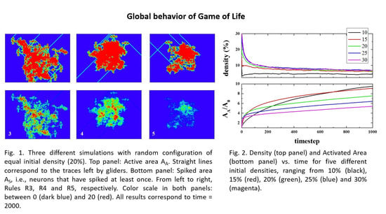
Starting from random initial conditions, “Life” will evolve through complex patterns, eventually settling down to a stationary state composed of different stable configurations, both static and periodic (see Figure 1). Despite its simple algorithm, the GoL simulates the dynamic evolution of a society of living individuals, including processes such as growth, death, survival, self-propagation, and competition. A class IV CA quickly produces apparent randomness, which is consistent with the tendency towards randomness observed in Brownian motion [36].

Let us examine a few characteristics of the GoL: Simulations can be carried out in open, closed, or periodic boundary conditions. In the present work, open boundary conditions were utilized, unless otherwise stated. Starting from a random initial distribution, life evolves to a final state composed of small stable clusters (see Figure 1 and Video 1 in the Supplementary material), usually blocks, blinkers, beehives, and others less likely to appear (see

Table 1. The most common clusters found in the GoL. Columns: Name of object, Size (number of live cells per object), Period (0 means no period exists), Heat (number of changing cells), Influence area (all cells which are in the Moore-neighborhood of each live cell of an object).

Name	Size	Period	Heat	Influence
Blinker	3	2	4	21
Block	4	1	-	16
Beehive	6	1	-	26
Loaf	7	1	-	30
Glider	5	4	5	22

). An important entity is the “glider”. In the GoL, there also exist configurations which "move" uniformly across the grid, executing a cycle of a few internal states. The simplest example is the glider that contains five live sites (Figure 1, Inset) and undergoes a cycle of length four.

Empirical investigations suggest that the density of structures containing L live sites generated from a disordered initial state decreases like e^l/L, where l is the size of the minimal distinct configuration which evolves to the required structure in one time step [43]. The time needed for the system, when N is large, to reach equilibrium is approximately equal to N, N×N being the size of the box. This is not true for special small configurations, as we will discuss later. The final density of life is small, independent of the initial one, unless the initial density is very small or very big (then life disappears completely) [44].

How Life resists noise was studied as early as 1978 [45]. In Schulman’s work, the GoL was studied including a stochastic element (that was called "temperature"). The idea was to examine how the introduction of a stochastic element in the local evolution rule would perturb the long-term evolution of the system. Temperature, in their study, was represented by the random perturbation of cell states as the rule was iterated. Then, the statistical properties examined were the density as a function of temperature and the (suitably defined) entropy. A phase transition was observed at a certain “Temperature” and certain "thermodynamic" constant of the motion [45]. A different approach was adopted in Reference [36], wherein by introducing stochastic rules in the GoL, it was found that ‘‘Life’’ exhibited a very rich critical behavior. Discontinuous (first-order) irreversible phase transitions between an extinct phase and a steady state supporting life were found [36]. A statistical analysis of the GoL can be found in Reference [46]. In that study, the number of clusters of n live sites at time t, the mean cluster size, and the diversity of sizes among other statistical functions was given. The dependence of the statistical functions on the initial density of live sites was examined as well.

Recently, dynamical aspects of CA have been studied by analyzing various characteristic parameters used in network theory [47,48,49]. The effect of network topology, i.e., the links between cells, on the evolution of the GoL has been studied using a version of the GoL on a 2D small-world [50]. The effect of synchronicity has also been examined in different studies [51,52,53].

For example, in Reference [52], the authors claim that an asynchronous GoL simulates exactly the behavior of the GoL in terms of universal computation and self-organization, no matter whether the update of cells is simultaneous or independent, according to some updating scheme like a time-driven [54] or step-driven [53] method. An abrupt change of behavior in the asynchronous GoL was presented in the work of Blok and Bergersen [53]. The authors showed that the phenomenon was a second-order phase transition, i.e., the macroscopic functions that describe the global behavior as a function of synchrony rate α (when α = 1 we have the classical synchronous updating and the system is deterministic, for α < 1 the system becomes stochastic) are continuous but their derivatives are discontinuous at the critical point α_c∼0.9. The critical threshold α_c separates two well-distinguished macroscopic behaviors or phases. The phase α > α_c is the frozen phase, in which the system evolves with low-density patterns and quickly stabilizes to a fixed point. The second phase (α < α_c) is the labyrinth phase, characterized by a steady state with higher density and the absence of stabilization at a fixed point [53]. Further research of the behavior of the GoL under different rules, i.e., different intervals of survival and fertility can be found in Reference [55]. However, all this complexity must not be confused with chaos. The GoL is not a chaotic system, it is deterministic but extremely complex. Life is not at the “border of chaos,” but thrives on the “border of extinction” [56].

The list of mentioned works does not claim to be complete. It only presents some important studies regarding different aspects of the GoL which could be of importance in our model as we will discuss later. In the presented work, to present our ideas, we utilized the original 2D GoL without any modification to either the topology or the synchronicity. To the best of our knowledge, almost nothing has been published connecting the GoL to brain dynamics, except for the work of de Beer [57,58].

3. The Basic Idea of the Model

The human brain comprises of a set of 10¹⁰–10¹¹ individual neurons and the total number of connections is even larger because every cell projects its synapses to a total of 10⁴–10⁵ different neurons [59]. With such an immense number of connections, our model is not intended to accurately describe the human brain or any other real nervous system, but rather to examine overall properties of a big connected group of discrete “neuron-like” elements. As a first approximation, we can assume that live cells in the GoL correspond to active neurons and dead cells to inactive neurons. As such, if the cells in the 2D grid are assumed to be single neurons, then the model may be considered unrealistic, since usually, a single neuron is connected on average to 10,000 neurons, and not only eight. This can be modified easily; counting second NN (the second ring around the cell) cells would have 24 connections, counting third NN cells would have 48 and so on, but that would make the model much more expensive, computationally speaking. To count 100 connections, it would be necessary to consider up to 15 NNs, for 1000 connections it would be necessary to consider 49 NNs.

More importantly, the resulting GoL differs significantly from the original Conway’s GoL. Another possibility is to assume that a cell in the simulation corresponds to a number of neurons (how big or small is an open question), or the other way around, that a number of cells (again, how many is unknown) correspond to a single neuron. For example, in the model proposed by Hoffman [10] the cells in the simulation represent small groups of neurons in the cortex. A cell in our simulation could be considered to represent, for example, a thousand neurons and that the neurons there, contained in a single cell, are connected with the other 8000 neurons around. This may look artificial but raises the first interesting question: Would a “large” (1000 or more) number of neurons interact, on average, with neighboring groups of the same size in the way that is modeled by the GoL?

In any case, despite the crude oversimplification, our question may be reformulated as: Is there any magnitude or measurable property in brain dynamics that behaves, on average, or presents some similarities with the GoL outputs? It must be noted at this point that all presented simulations (unless otherwise stated) were performed for randomly generated initial configurations in a 1000 × 1000 square box, with open boundary conditions, and the presented results for each different configuration were averaged over 20 simulations. 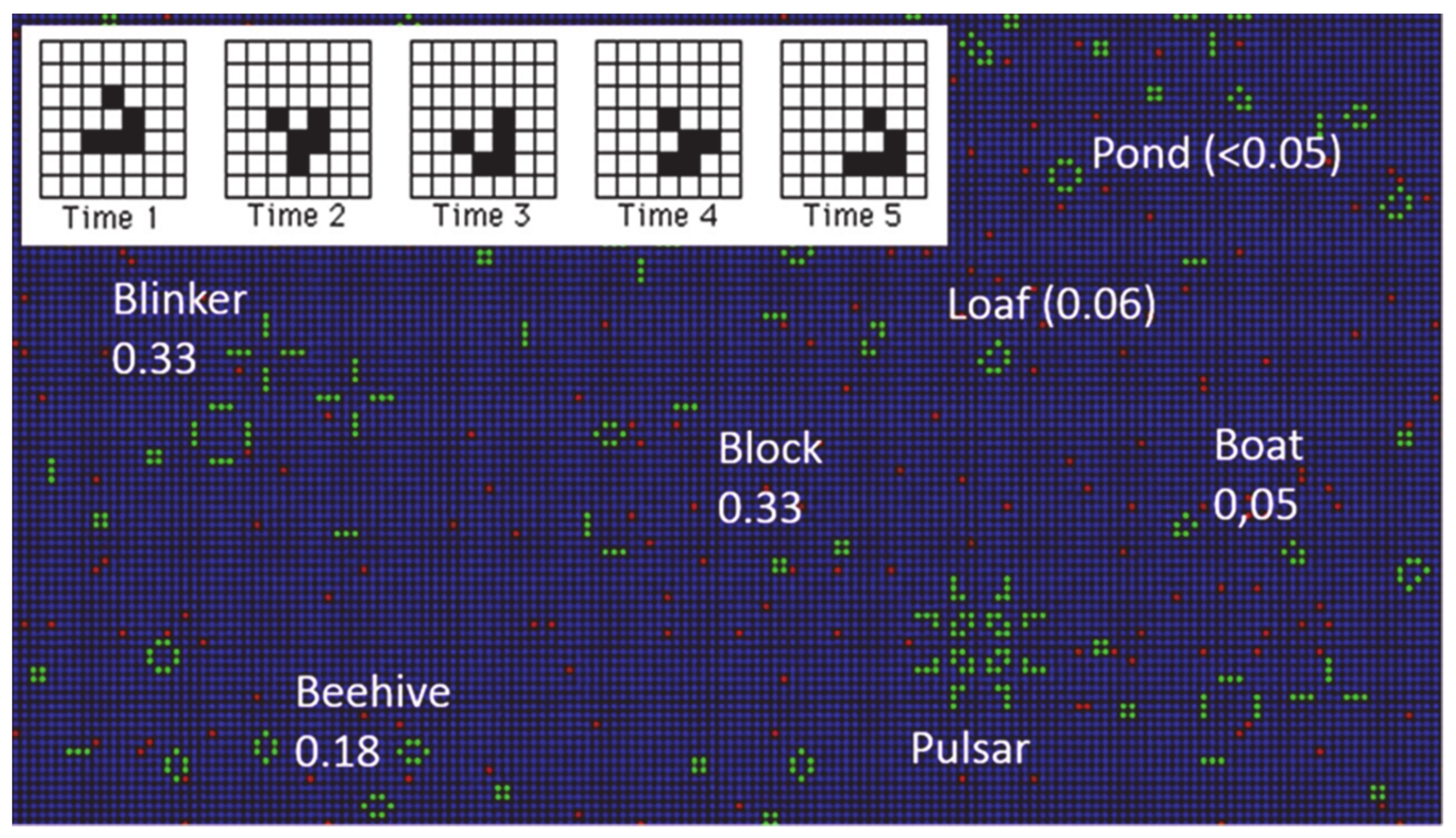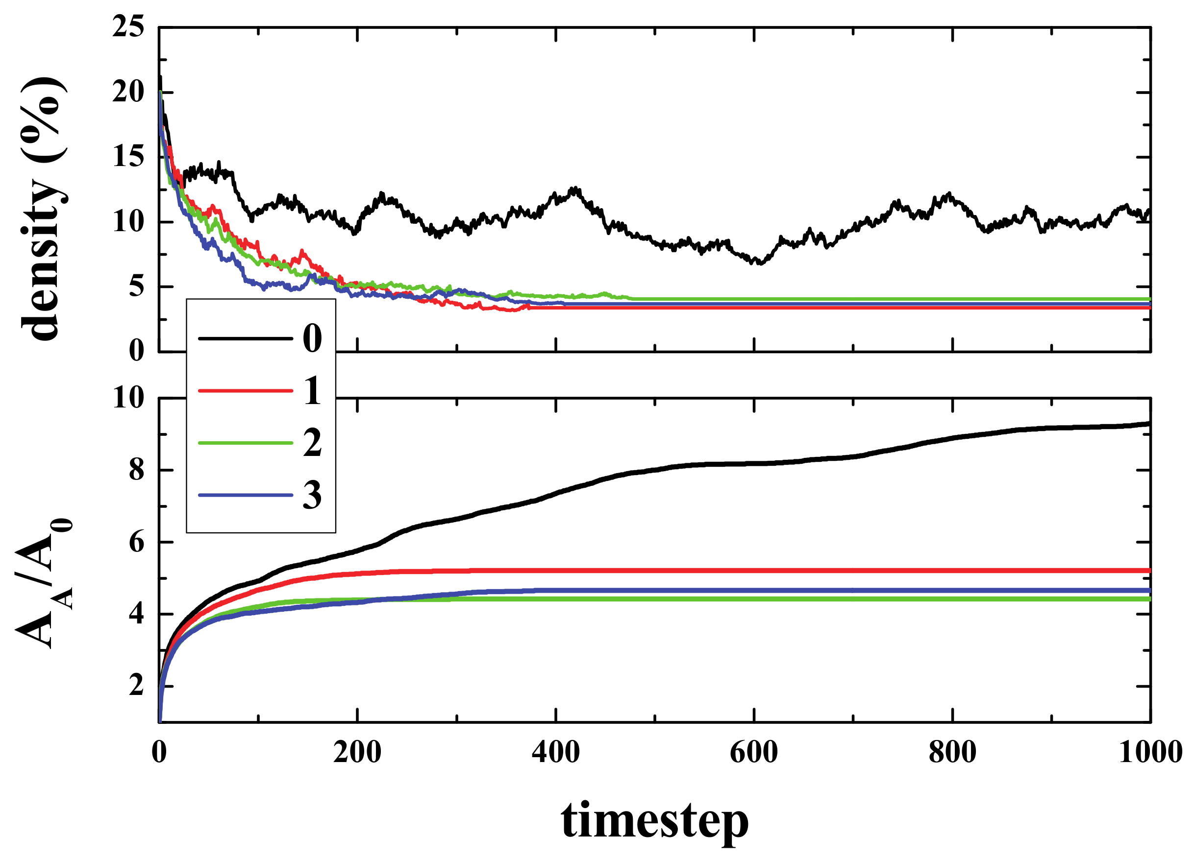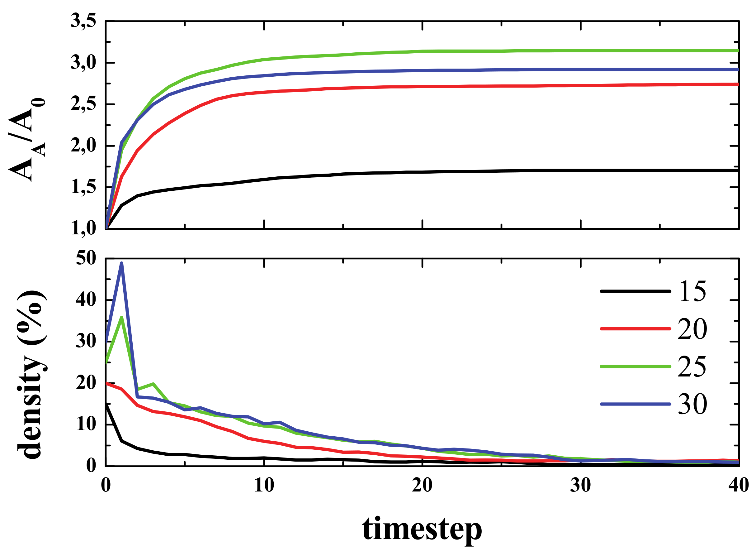Figure 2 (top panel) shows the time evolution of density (i.e., the number of live cells divided by the total number of cells), starting from different initial densities. As can be seen, in a few steps (100), the density of life decreases very fast (almost exponentially) to a lower density that then decreases to a final value of ~2.7%, independent of the initial one. The exact way in which density decreases is, to the best of our knowledge, unknown. The curves, in the first 100 steps (approximately), can be fitted to an exponential decay.

The lower panel shows the normalized Activated Area, A_A/A₀ where A_A is the area in the simulation that has been active at least once, and A₀ is the initial active area (the initial number of live cells). The Activated Area grows faster for high densities (initial density ρ_i ≥ 15%) only during the first stages of the simulation (for times ≤ 500). After this first stage, the slope decreases, whilst for ρ_i = 10%, A_A continues growing with a similar slope. Hence, for the activated area, two stages can be differentiated in the evolution of the system. Initially, the area increase occurs at a fast rate, and then, after some time τ(ρ_i), the rate of increase becomes slower. It is important to note that the ratio of A_A/A₀ is > 1, but that does not mean multi-counting. When the activated area is computed, we count the cells that have been alive at least once. However, when a cell is counted, then it is no longer counted again. That is to say, if a cell is alive at time 0 (or time x), it is not counted again if it goes back to life at time n (> 0 (or > x)). The idea is very much like the random walk study presented in Reference [60]. The reason to have a ratio > 1 is that we start, for example, with an initial density of 10%, i.e., 10% of the initial area is active. If this is the case in a closed simulation, then the ratio can be as high as 10 at a certain time (and unlimited in an open (infinite) simulation). As for the reason to define the activated area in our model, there are studies where the spatial extension of brain activity is studied [61,62].

Clearly, a one-to-one comparison of our model to real brain data would be highly desirable. However, that is not the main goal of this study, but rather it is to create a simple framework (with high complexity at the same time as we will see) capable of being used as a model of brain dynamics. Comparing the activated area, signal transmission, etc., as defined in our model to real experiments (EEG, fMRI, etc.) requires further study and collaboration with neurologists.

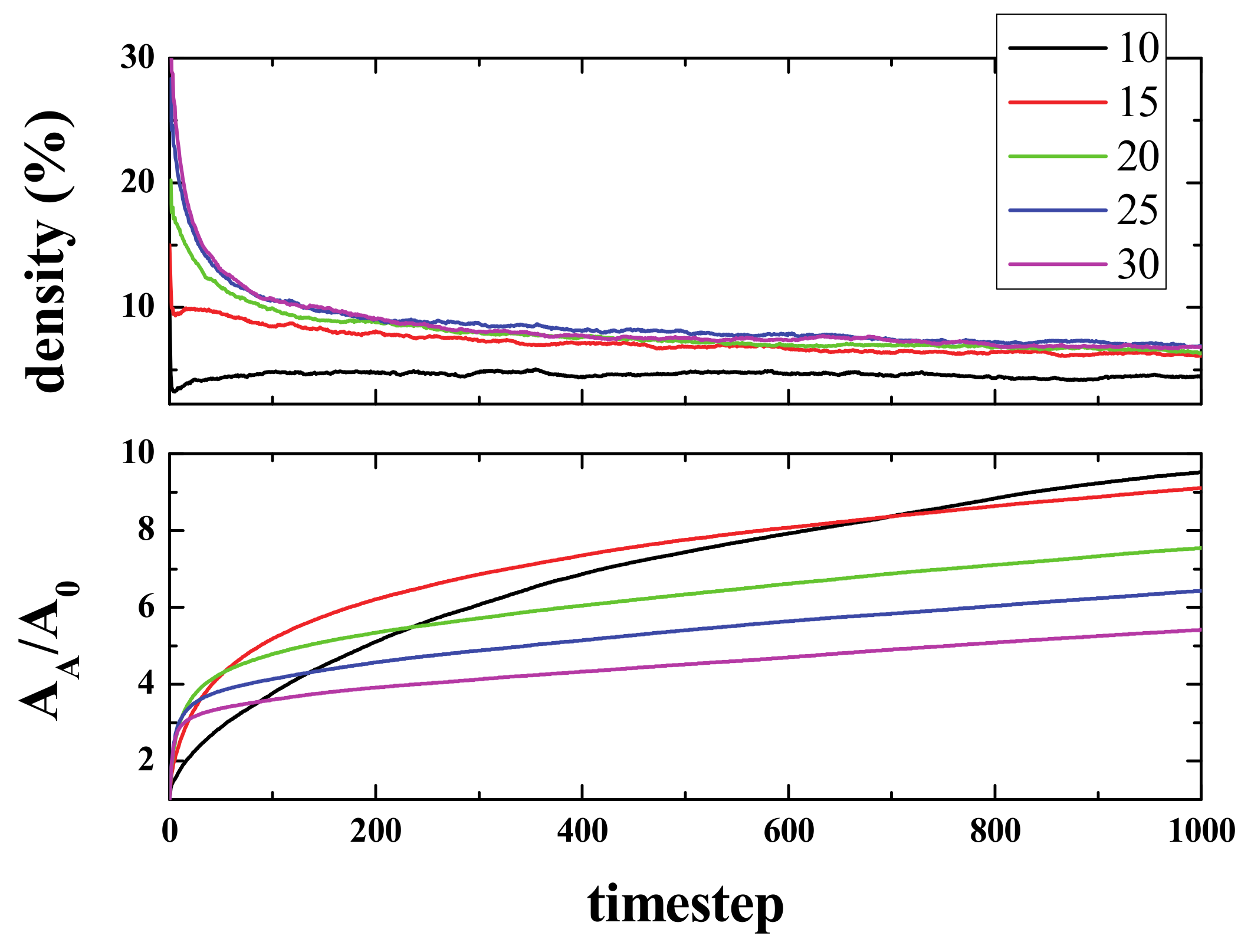
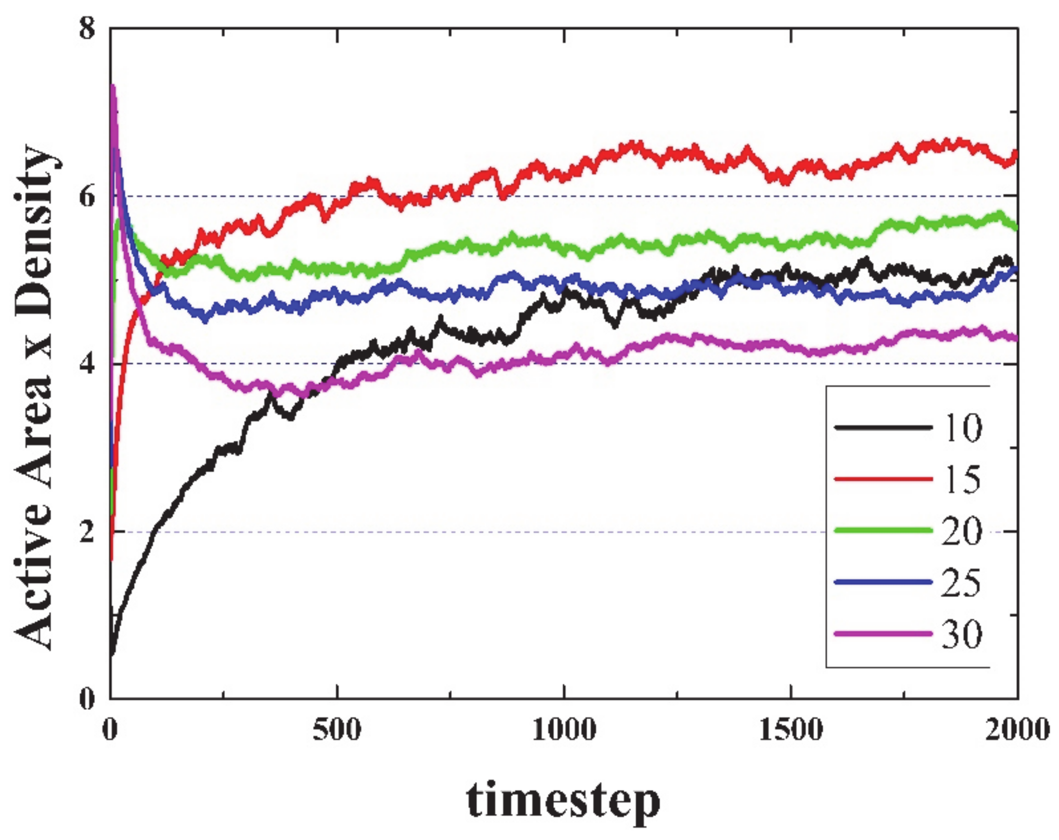
At this stage, an interesting conclusion may be drawn: The maximum/optimal spreading of activity in the grid is achieved for initial densities between 10 and 15%. Figure 2 suggests a very likely conjecture: “For large enough sample sizes and long simulation times, on average, the product Density times the Activated Area remains constant for all initial densities”. To illustrate this idea, Figure 3 shows the product Density x Active Area versus time. Note that this conjecture cannot be true in open simulations (infinite side), since the area can grow endlessly (due to emitted gliders moving away from the initial live cells), but density will reach a constant value (or equilibrium value).

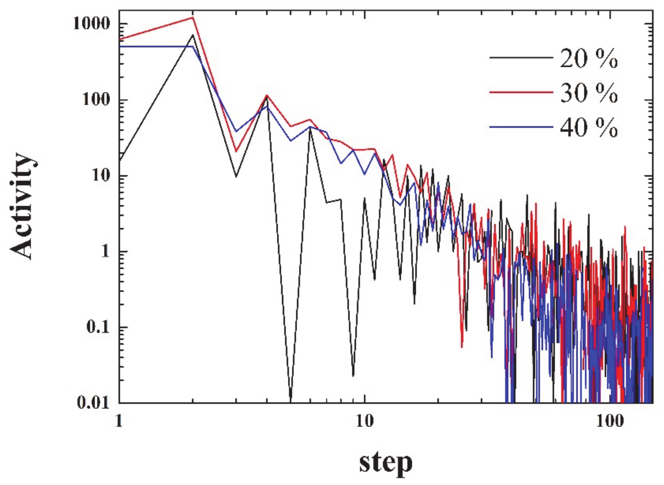
The activity can be defined as:

X = [ρ(t) − ρ(t − 1)]²

(1)

i.e., as the squared difference between consecutive densities. As seen in Figure 4, the activity decays more than three orders of magnitude within the first 100 steps. The figure is noisy, since it has not been averaged over a number of simulations.

Despite the possible answer to the previous questions, a possible first idea is to use a random distribution of neurons, some active and some inactive, in an open grid, and since in the final state some neurons will be active far from the initial ones, associate the simulation to an impulse or stimulus that is originated somewhere (the initial configuration) and evolves temporally. We can study how the “information” or the activity spreads (since is difficult to define information). 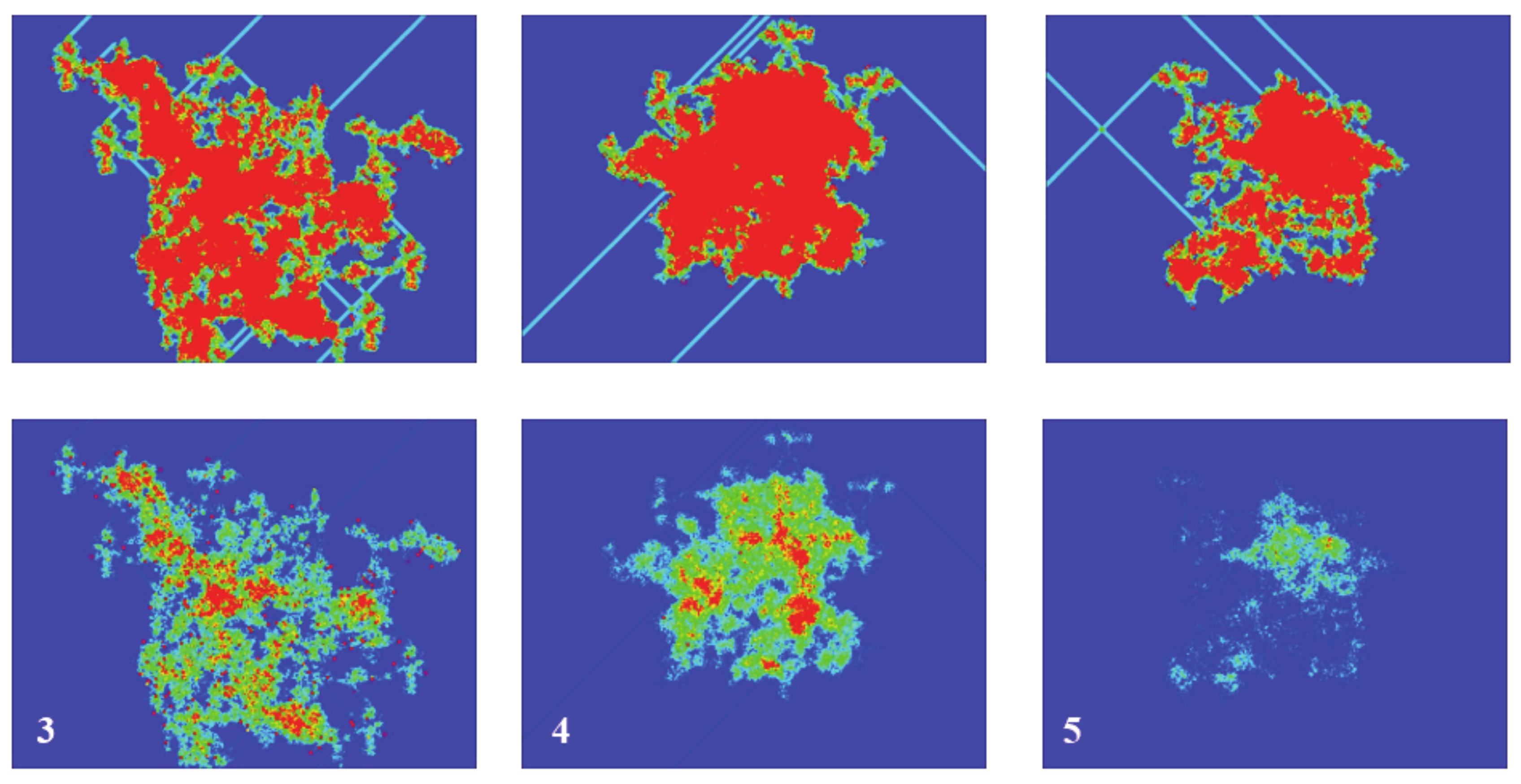Figure 5 (top panel) shows an example, in order to make this clearer. It presents the spreading of activity for the same initial density (20%), but different random starting configurations, after 2000 timesteps. The color scale corresponds to the number of times that the cells have been active during the simulation. For the sake of clarity, the scale has been limited between 0 (dark blue) and 20 (red), meaning that a red cell has been active during at least 20 steps. As can be seen, the activity spreads from the initial emplacement in a “random way”. The total number of cells that are active (no matter how many times) for a given time will be called the “activated area” or “sampled area”. This area will vary from one simulation to the next, both in size and shape, as can be seen in the three presented examples. It must be noted that there exist spots on the grid that have been active for a total time that can be very close to the total number of steps, which can be the case of a stable configuration formed at the very beginning that did not interact again with the rest of the system. The bottom panel of Figure 5, which refers to spiking activity, will be discussed in a later section.

To be precise, the simulation may be terminated once the density becomes constant, or when the “sampled area” reaches a final constant value. By choosing the second option, this can lead to an infinite number of steps and a never-ending simulation, since gliders appear quite often, which would lead to a non-stopping increase of the sampled area if they move away from the center of the system. In our analyses, we neglected the fact that the system was still active due to the presence of gliders (or any other “ships”), and we defined equilibrium as the time after which no more changes are observed in the system, except for the periodic ones due to blinkers and similar clusters.

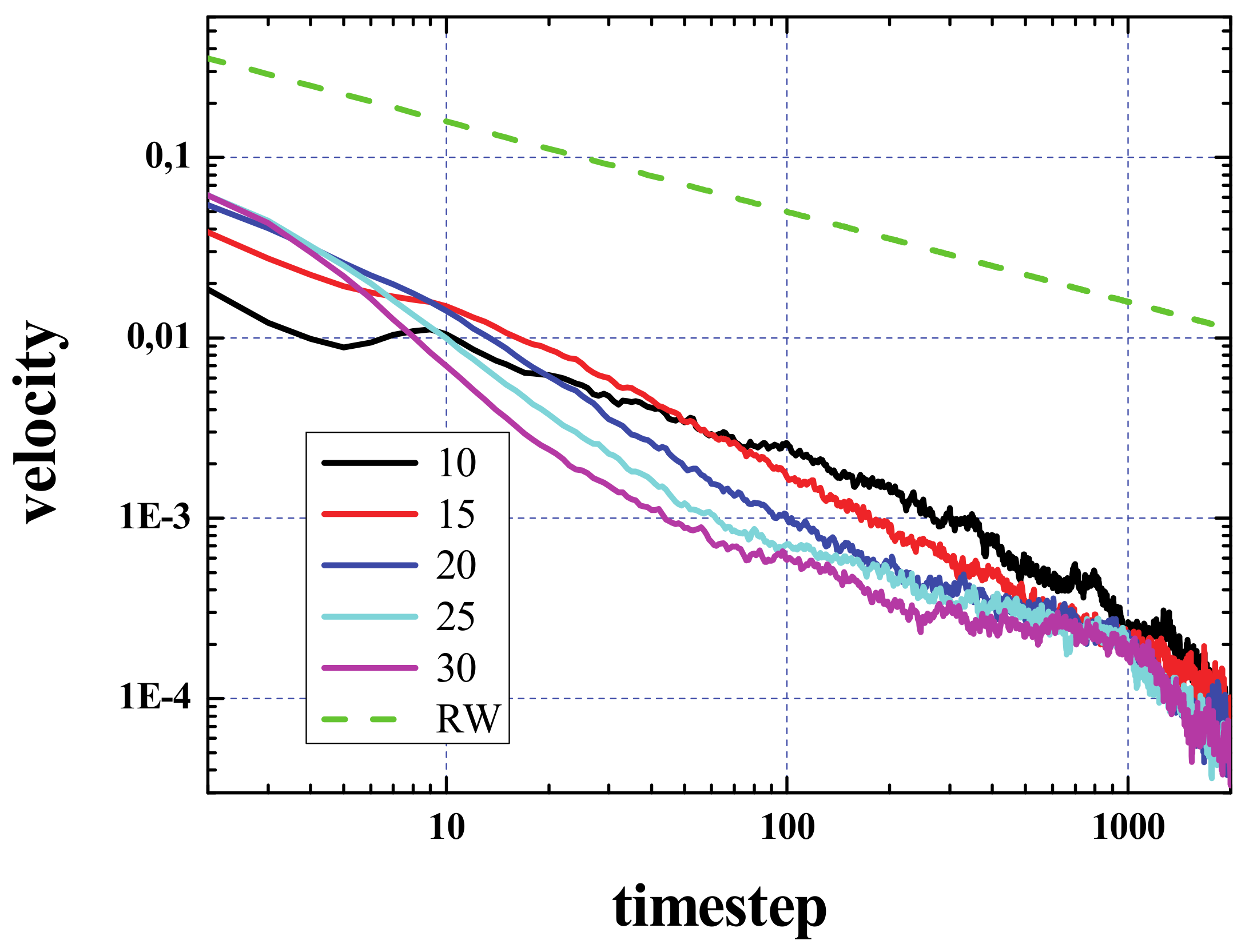
Thus, we can study how far and fast the signal (or activity) spreads. As a first approximation, the activated area (considered a circular one) can be written as πr²(t) (r being the distance from the center of the box), hence we can write the velocity of the spreading signal as:

$$v\left(t\right)=\frac{1}{\sqrt{\pi }}\frac{d\sqrt{A_A}}{dt}$$

(2)

Figure 6 shows the velocity calculated from the curves of the activated area vs. time, presented in Figure 2. For comparison, we have also plotted the result considering the spread as a pure random walk (green dashed curve).

It has to be noted that the activated area will increase outwards as well as inwards. The velocity of the signal propagation calculated from the increase of this area as a circle that grows from the center of the initial configuration is only valid after the area of the box containing the initial configuration has been sampled. This occurs for values of time that depend on the density and is about a few hundreds of steps. In the very first steps of the simulation, a big increase of this area is expected, since, grosso modo, most of the dead cells around the living ones will become live in few steps, so that the activated area will increase from A₀ to 2A₀, 3A₀, etc., in only a few steps. At the same time, as has already been discussed, in few steps the density decreases, and this process is fast as well (see top panel of Figure 2), so that in a few steps the increase of the initial active area will not be “explosive” anymore.

This simple computational experiment could be the first step towards answering a number of important questions and determining whether the GoL is a suitable model. How does a signal propagate in the brain? Is there experimental data that might relate to this simple model of neuronal activity? Can we define the initial configuration as an impulse or stimulus (in microvolts, with the density determining its range for example), and its subsequent evolution as the spreading of that signal or information?

Moreover, it has been argued that in the brain, volume conduction (or electrical spread) is a passive resistive process, where the amplitude of the extracellular signal decreases as the distance from the active membrane increases, as described in Reference [63] (see Figure 1 and Figure 3 in that paper). This is not an argument to verify our model; however, our model presents similarities, since the signal propagates fast around the initial activated region and slowly far from it. In the CA model proposed by Hofmann, the excitation of a region of space does not propagate to distant regions [10], this is also true of cortical regions under normal conditions [64]. Similar behavior is predicted by our model.

The activated area, A_A increases from A₀ to 10 to 15 times A₀, which means that the initial square is filled (i.e., A_A is multiplied by a factor 100/ρ_i) and then little spread is observed. In terms of the initial size, N×N, the final activated area (or sampled area) would be less than 2N × 2N, so that the signal (neglecting the propagation due to gliders that will continue growing forever) is not spreading more than N cells from the borders of the initial distribution. However, this is something that may vary from one simulation to the next, and it is certainly not true for special configurations such as the “Methuselahs,” as we will discuss later.

The first possible connection of the presented model with brain dynamics is shown at this point. We compare the spreading of activity with the cortical spreading depolarization (CSD) wave [65]. Spreading depolarization waves of the neurons (and neuroglia) propagate across the gray matter at a velocity of 2–5 mm/min, [66,67], i.e., 0.33–0.83 × 10^-4 mm/ms. If we calculate the velocity of growth of the active area during the first 100 steps, when A_A grows fast, it is found that V = 10⁻³–10⁻⁴ cells/step. If we assume that the timestep is in ms, in accordance to Reference [68], and cell size is of the order of mm³, then V is predicted to be higher than that of the CSD by one order of magnitude. To make this comparison, we have assumed a one-to-one correspondence between neurons and cells in our model. However, since the number of actual neurons represented by each CA cell is a user-defined parameter, in that sense the CA model is flexible and can achieve better agreement.

It has to be noted that if each computational cell is assumed as a single neuron, there exists some ambiguity, since the size of neurons is not constant but depends on the type of neuron, etc. For instance, pyramidal cells are big (~20µm), whilst stellate cells are smaller [69]. Moreover, CSD is not the only measurable quantity that exists in brain dynamics and other phenomena may be modeled. For instance, during an epileptic crisis, the rate of migration of hypersynchronous activity (hallmark of epilepsy) has been experimentally recorded and the estimated value is about 4 m/ms, [70,71], i.e., approximately 60 times higher than that of the CSD.

4. Spikes in the GoL Model

Inspired by the Wilson-Cowan model [72,73], we defined spikes in a similar manner. Most neurons require a minimum level of input before they fire. That threshold in our model can be the number of adjacent active cells. In this way, a cell (neuron) spikes when it is active and has exactly x number of active neighbors. We will refer to spiking requirements or rules as R3, R4, R5, and R6, with 3, 4, 5, and 6 being the previously defined number x. In each case, a cell is considered as having had spiking activity if it has spiked at least once, obeying either of the previously mentioned spiking rules. In this way, similar to the active area, the spiked area A_S may be defined at each timestep as the total number of cells that have spiked at least once (obviously, A_S as A_A can never decrease). It is a well-known fact in neurophysiology that the same neuron can become inactive and active (firing) many times per second [72,73]. Regardless, real neurons have a period of refractoriness after which they can fire again. This period last about 15 milliseconds and in our model, we assumed that this discrete timestep corresponded to the discrete unit of time.

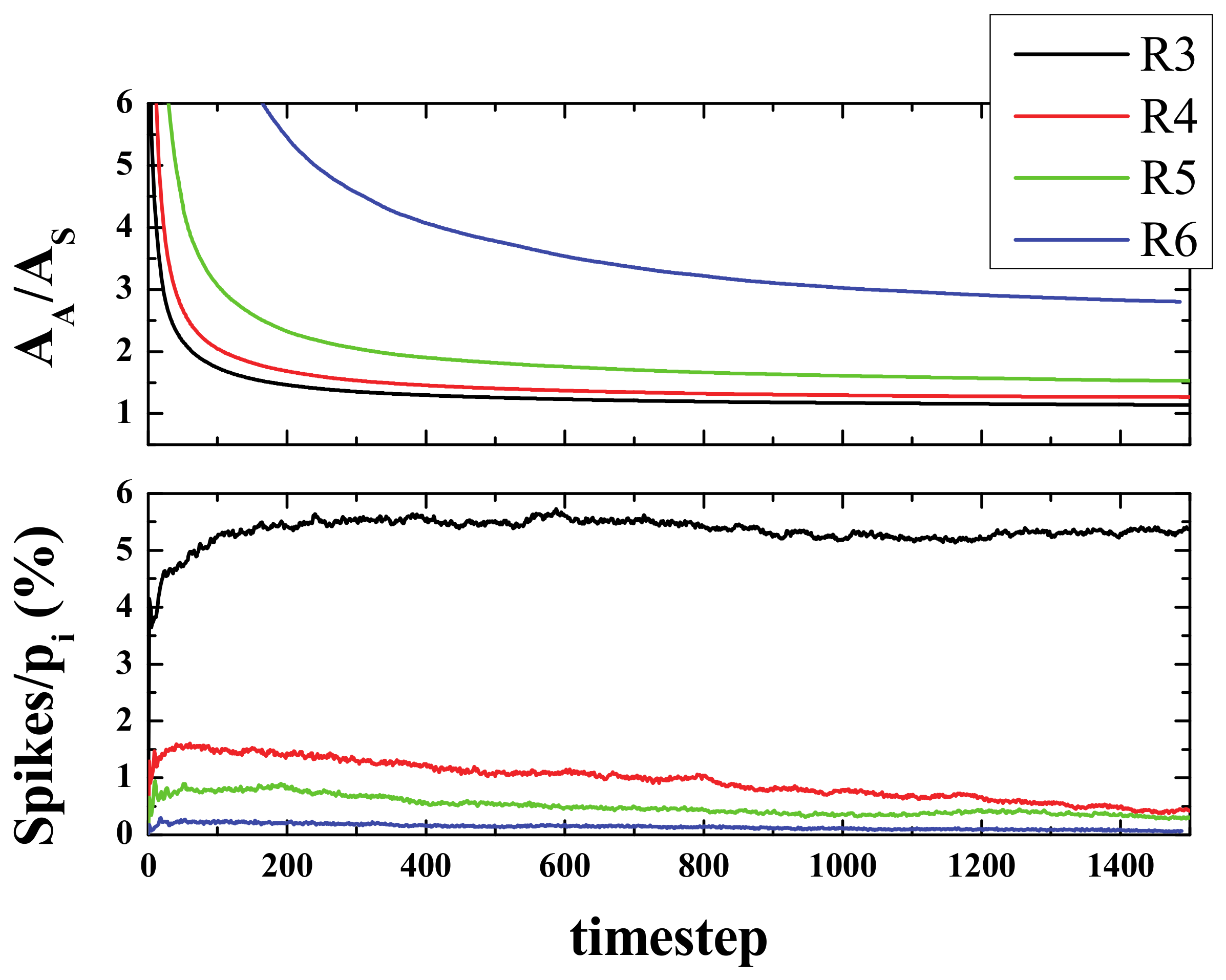
Please note that in the W-C model, the neighborhood includes only 4 cells (von Neumann neighborhood), whilst in our model it included eight (as in the classical GoL model). Moreover, in the present version of the model, there is no differentiation between excitatory and inhibitory neurons. Obviously, these conditions could be easily modified. A simulation was carried out, where a randomly distributed initial density of 20% (i.e., 200,000 active cells in a 1000 × 1000 grid) was left to evolve, following spiking rules R3, R4, R5, and R6), and the spiking activity was measured. The averaged results of 20 different simulations for each rule are presented in Figure 7.

The spike curves prove helpful in understanding the evolution of the system. The number of spikes for a given time are the number of active neurons that have exactly 3, 4, 5, or 6 active neighbors at that step. Since we started from a low-density configuration (ρ_i = 20%), at the very first stages, the number of spikes was found to be small in terms of the initial area (or initial population pi) and it grew, but not by much, within a few steps (less than 10). Then, after this initial reorganization, an almost flat curve was observed, especially for rules R4, R5, and R6. The average value for the first 200 steps after the aforementioned reorganization (from 20 to 220 steps) was as follows: 5.15, 1.48, 0.80, and 0.22 for R3, R4, R5, and R6, respectively (see bottom panel of Figure 7).

The ratio A_A/A_S converged fast to an almost constant value for R3, R4, and R5, but not as fast for R6. For R3 and R4 the ratio was almost 1, i.e., the spiked area becomes almost equal to the active area. However, the number of spikes with the R3 rule was more than 5 times larger than the one with R4. For R5 that ratio was 1.5 and for R6 the ratio was approximately 2.5 (see top panel of Figure 7).

Returning to Figure 5, its bottom panel presents the results of the spiked area A_S at timestep 2000, for three simulations with a random initial configuration of density of 20% in a 1000 × 1000 grid and spiking rules R3, R4, and R5, respectively. The top panel presents the respective active areas (as has already been discussed) and the colors for the sake of clarity have been limited between 0 and 20. The shape and size of both areas (active and spiked) vary significantly between different simulations, a fact arising from the different initial random configurations. However, the ratio A_A/A_S has not changed and remains almost constant at 1 for R3 and R4 and 1.5 for R5, as discussed in the previous paragraph.

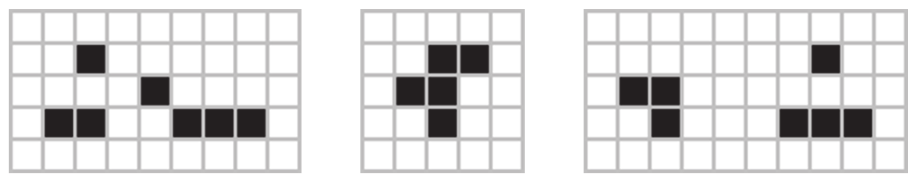
From the above analyses, one could deduce that starting from a small community of live cells, let us say less than 10 or 20, the system would reach equilibrium in a few steps. However, this is not the case for some configurations called "Methuselahs" [74]. Some well-known Methuselahs are the acorn, the r-pentonimo, and the diehard. These apparently simple configurations (and their subsequent evolutions) are good examples of the amazing complexity that can be found in the GoL. Figure 8 shows the (a) acorn, (b) r-pentonimo, (c) diehard.

See Video 2 in supplementary material for a simulation involving the acorn. The acorn resulted in a stable configuration after approximately 5000 steps. Starting from an initial configuration of the acorn at the center of the box (only 7 cells live), the stable pattern that emerged contained 633 cells, and the total sampled area was around 22,885 cells (a small part of this area accounted for the area sampled by some gliders before the system reached equilibrium). Using the acorn as a starting point, we examined the evolution of the spiking area under different spiking rules. 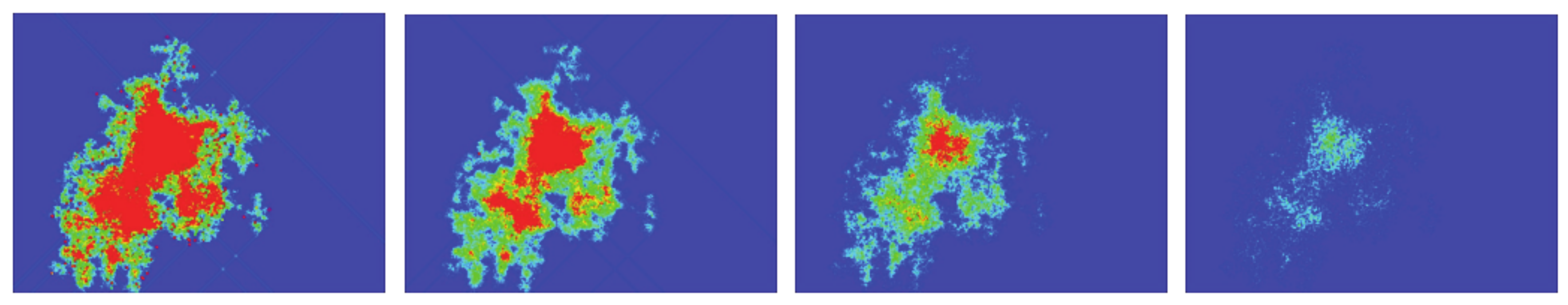Figure 9 presents the spiked area (for cells that have spiked at least once) at a timestep of 2000, for spiking rules R3, R4, R5, and R6, and as expected, the spiked area is lower when the number of neighbors required for a neuron to spike is higher.

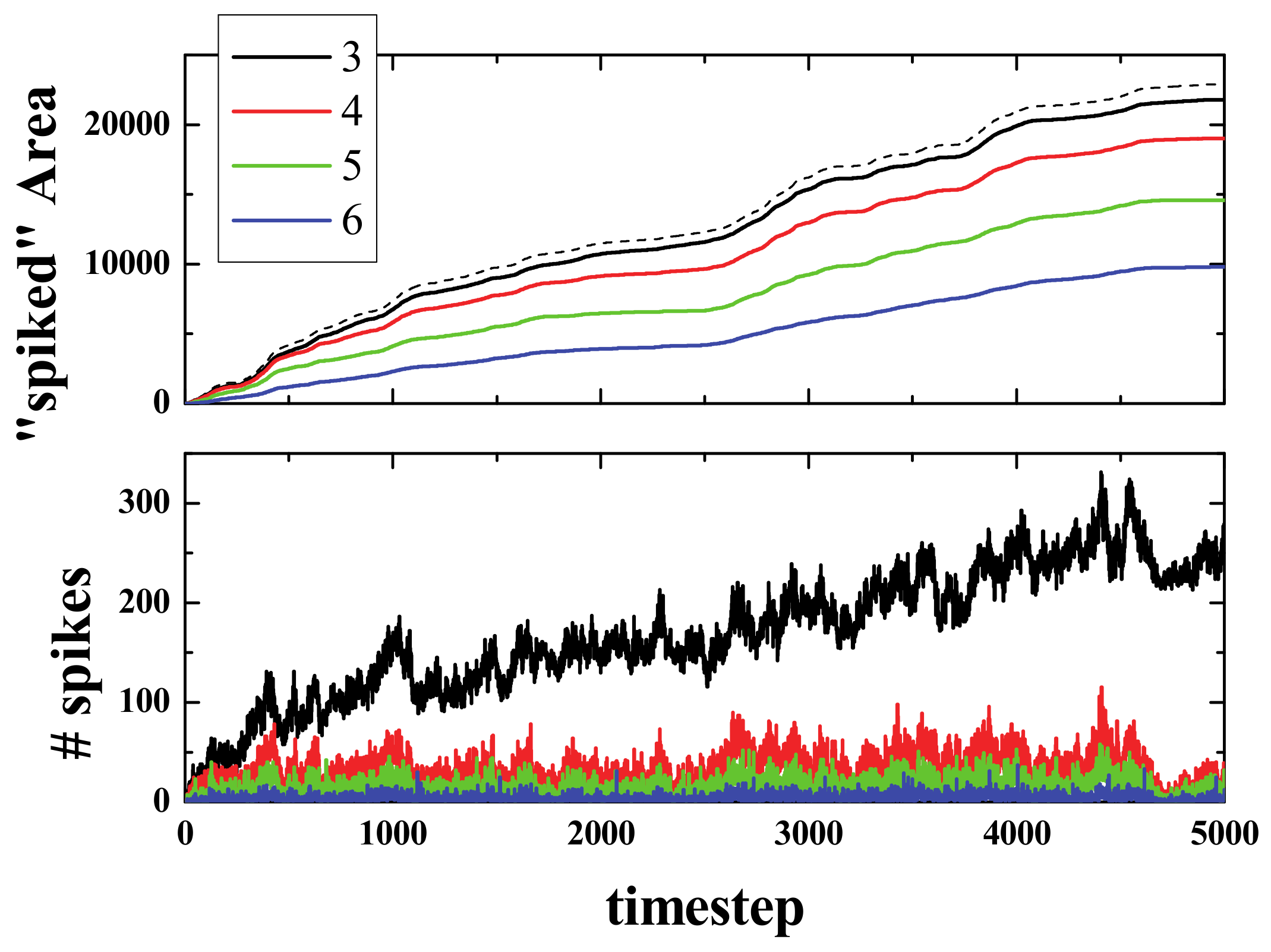
Figure 10 presents the results of the simulations for the acorn with 4 different spiking rules. As can be seen in the top panel, the spiked area for R3 (continuous black line) was almost equal to the active area (black dashed line), and then it decreased for the other rules in the expected order (i.e., R3, R4, R5, R6 from biggest to smallest). The bottom panel of Figure 10 presents the sum (from timestep 1 up to the current timestep) of spikes that have appeared for each of the 4 different spiking rules. As can be seen, the R3 curve exhibited, after the initial stages of the simulation, more than twice the number of spikes that the R4 curve did.

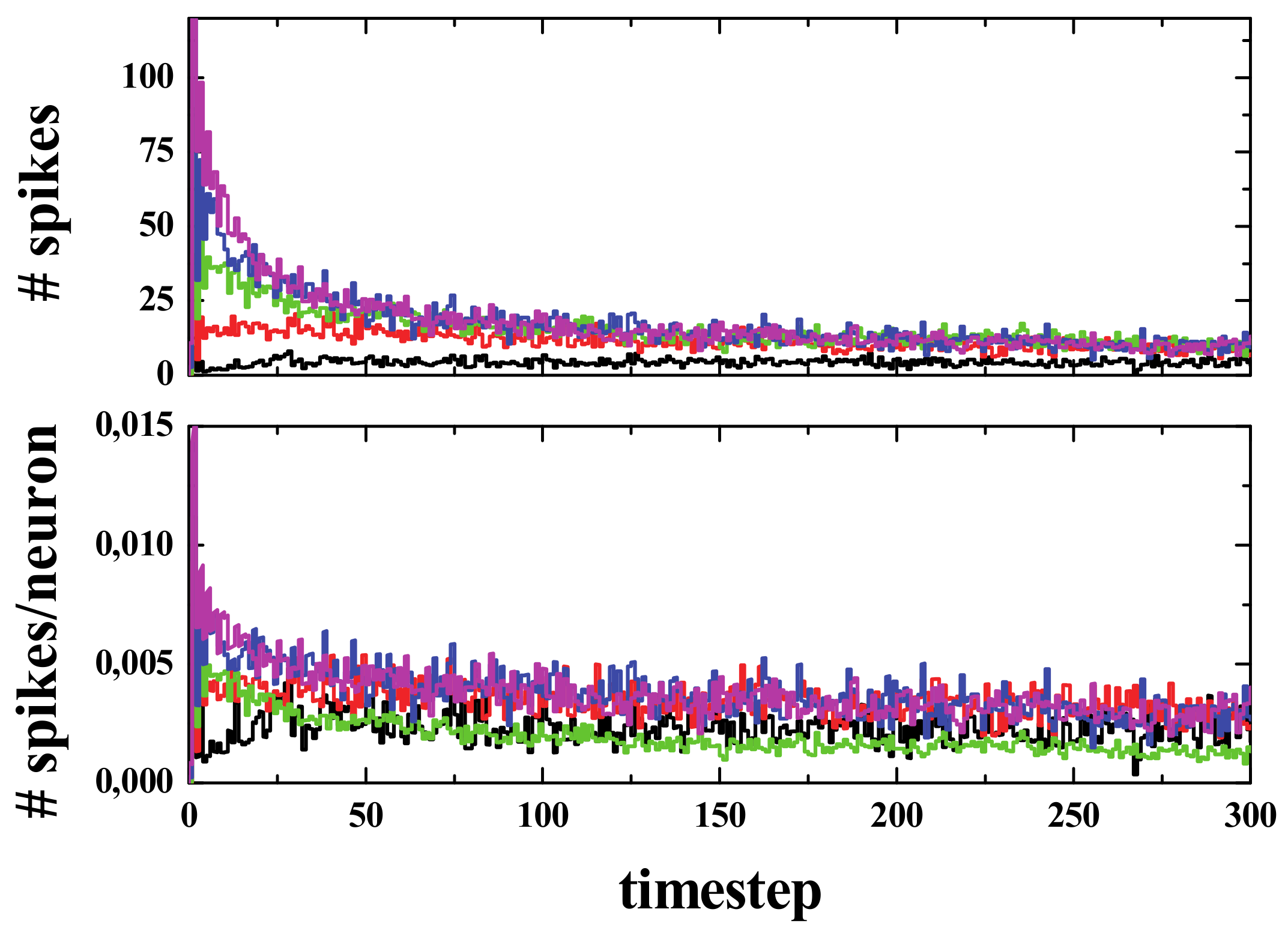
Simulating the acorn was interesting to show the expected differences once the spiking rule was modified; however, the results obtained using the acorn may be not valid in general. If the simulations were carried out with various initial random configurations with spiking rule R3, the number of spikes decays fast (see Figure 11, Top panel), and when the number of spikes is divided by the population (that decays exponentially), the resulting behavior of the spikes per neuron versus time is a small decrease in the very first stages of the simulation, only around the first 50 steps, as can be seen in Figure 11’s bottom panel, followed by an almost constant value in the next steps.

Apart from the very first stage of the simulation, we observed an average of 0.005 spikes (or firing neurons) per active neurons as time progressed. This can be compared to the results of a more realistic model like the one presented in Reference [68]. In that study (See Figure 2), the number of firing excitatory neurons is given. The value was about 400–500 firing neurons within a total of a million neurons, i.e., only 0.04–0.05%. It is also important to note that this result corresponded to a typical test with normal non-periodic behavior. Periodic states with high activity are associated with epileptic episodes [68].

Can this simple model of spiking activity be compared to real spiking activity in a real brain? How many spikes should we have per time and area? We have a certain number of spikes (per time, per area, etc.). It remains to be confirmed if this number is too low or too high compared to the usual number of spikes per neuron in the brain (or some part of it, depending on the activity).

5. Defects and Percolation

A simple ingredient that can be added to the present model is the presence of defects, i.e., cells that are inactive, neither dead nor alive, but are totally inactive all the time. These defects act as boundaries, i.e., they cannot become alive and are not counted when the GoL rules are applied. By doing so, we can study how these defects affect the propagation of life (i.e., a signal) as studied earlier. The basic idea or question behind this is: Is it possible to associate the presence of defects, defined in this way, to dead neurons that are present in neuronal diseases like Alzheimer or autism? [75,76,77,78].

We set up two communities separated by an empty space to study how the two communities mixed and/or interacted. In this way, we assumed that the two communities represented two parts of the brain (how big or small is an important question), which were somewhere disconnected (i.e., the part of the brain in between two active areas is in total rest state). We observed how they connected, i.e., we could define some kind of connectivity and studied this connectivity and its dependence to the initial density of active cells and other parameters.

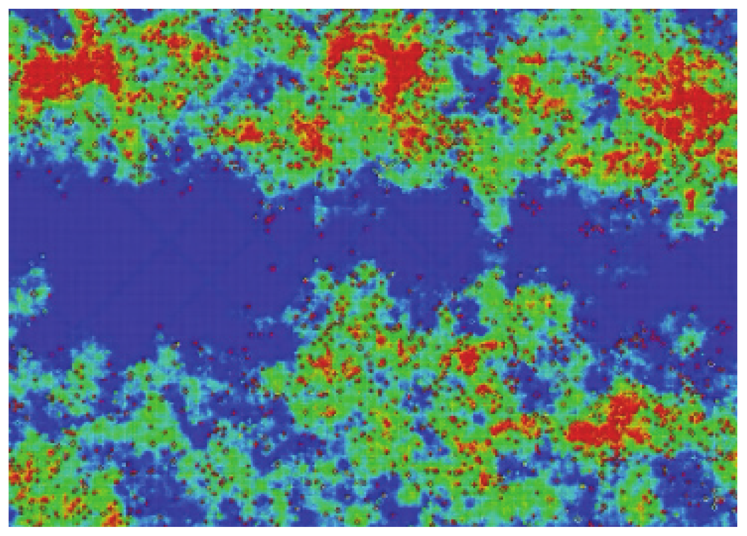
Figure 12 shows the result of one of our simulations of this interaction. The sample size N × M was 100 × 300 (vertical by horizontal), meaning that the empty space between the two communities (i.e., the gap), N/3, was 33 cells. The initial density was 20% in the top and bottom regions (33 × 300 cells each). In the presented case, the number of defects was 2% in the middle region.

As can be seen, after some steps (350 steps, 35 secs in the video), both communities interact. For clarity’s sake, when this occurs, we plotted the resulting “life” in yellow. A simple way to quantify the interaction is to study only the density of “yellow neurons,” as we will see later. Henceforth, the density of active neurons after the interaction of the two separated communities will be referred to as “mixed density.”

However, to analyze the effect of defects on the transmission of information or in the communication of the two parts of the “brain”, let us understand the effect on the transmission or propagation of life. If the simulation was run with an initial density of life plus a percentage of randomly distributed defects, what is observed is a clear decrease in the time needed to reach equilibrium. This can be observed in the density and active area curves, since both reach the final value in a few steps compared to the 0% defects case (See Figure 13).

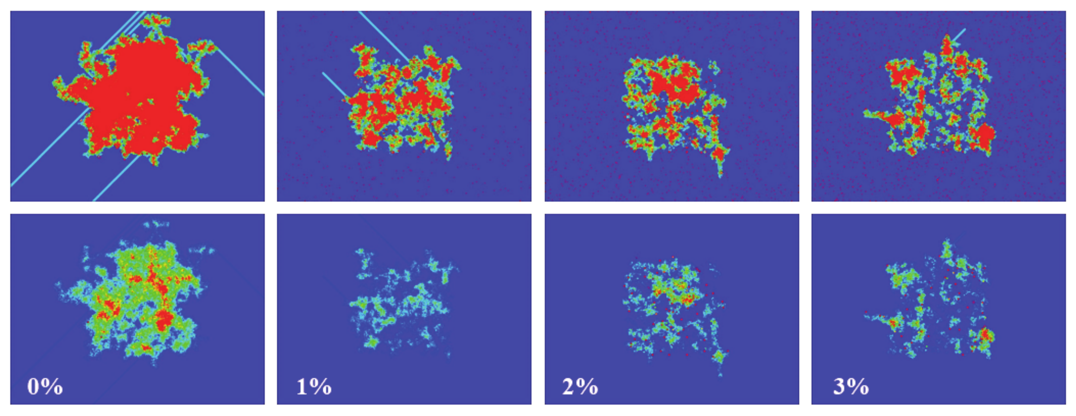
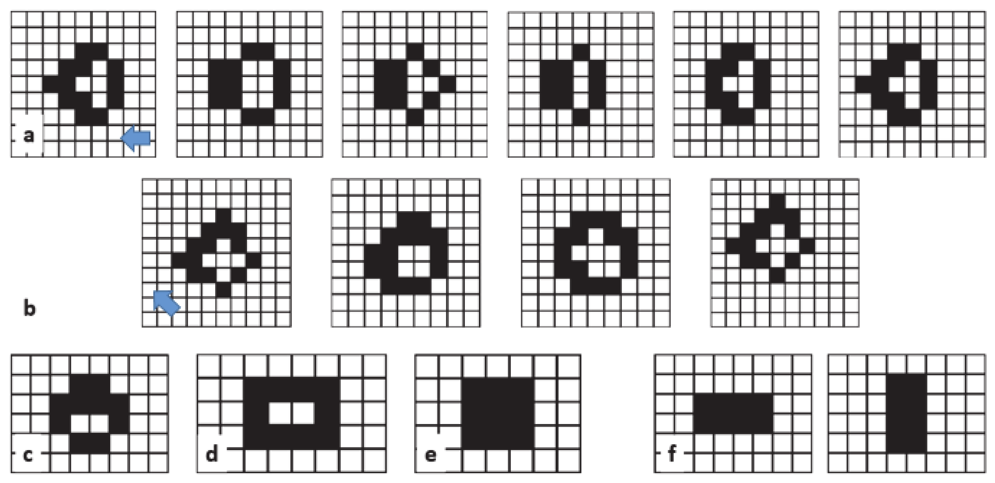
To show how defects affect the signal propagation, we presented four different simulations with an initial density of 15% in the center of the box, and with defects being randomly distributed across the computational domain. The percentage of defects ranged from 0% to 3% (from left to right, see Figure 14). As can be seen, the higher the number of defects, the smaller the activated area, and the same applies for the spiked area (bottom panel). In the top panel, it can also be seen how the defects block the paths of gliders (for 1% and 3% defects).

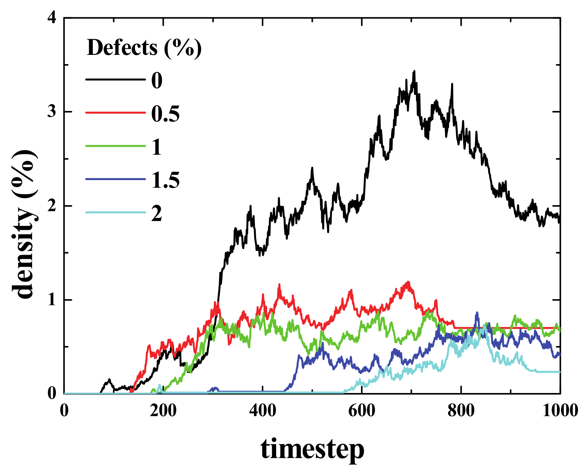
Figure 15 shows the “mixed density” for 5 simulations that were performed for two initially separated regions with initial densities, ρ_i = 20% each, for different densities of defects in the middle region (i.e., the same configuration as described for the simulations presented in Figure 13). The result was not absolute (or was relative) in two ways. First, it presented only single simulations and not averaged curves. For the same conditions, the results changed significantly from one simulation to another, and in some cases, both communities would not interact at all. The idea was to demonstrate that the lower the number of defects, the easier it becomes for the two regions (upper and lower) to interact (i.e., lesser time is needed for the mixed density to become different from zero). Moreover, the interaction becomes stronger, if we consider the area under the density curve as a measure of strength (See Video 4 in the supplementary material).

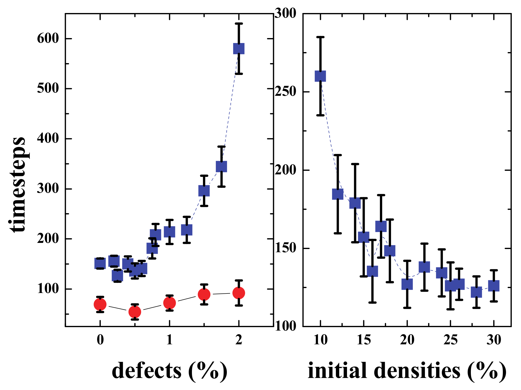
The connectivity was achieved in several timesteps that depended on the densities of the upper and lower regions (See Figure 16, right panel). For low densities, the time was larger, and then for densities ≥ than 20%, it was approximately 125 steps, the gap distance was 100 cells, meaning that the communities “moved” towards each other with a velocity v = 50/125 = 0.4 grid-cells/timestep. Then for a given density (20% in this case), the time needed to interact will depend on the percentage of defects present in the middle region (Figure 16 left). When the percentage of defects is less than or equal to 0.75%, the effect is almost negligible; however, for bigger percentages, the time clearly increases, and when the defects reach more than 2% of the grid in the middle region, the signal is almost blocked.

It must be noted that the values presented in Figure 16 are obviously geometry-dependent. As already mentioned, the sample size is N×M (vertical by horizontal). If the gap (N/3 in our simulations, though it can be any other fraction of N) is very big compared to N, the two communities are unlikely to interact, except via gliders (or other “ships”), and when the gap is small the interaction will be fast. Note that, as shown in Figure 14, the gliders may be hindered by a single defect. If the size of the two communities (in terms of the fraction of N) is not very big, then it is more unlikely to create “traveling groups” that will end up connecting both sides.

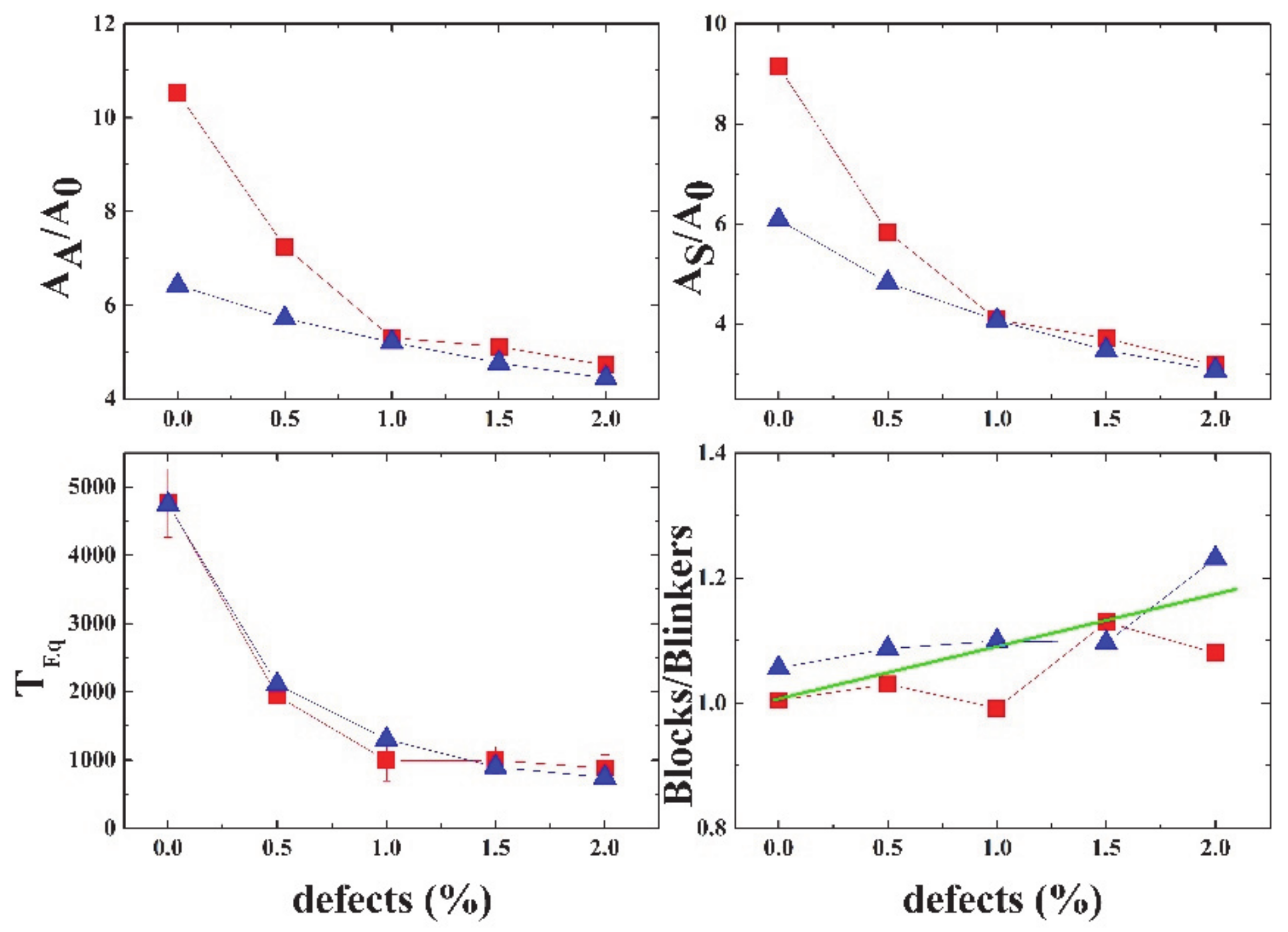
Figure 17 shows a summary of the different properties of Life, depending on the percentage of defects in the grid. The equilibration time decays exponentially with the percentage of defects.

In this part, we have established a second idea that deserves further study. This simple model with the addition of defects may be utilized to study neural network dysfunctions in the excitatory and inhibitory circuits that have been proposed as a mechanism in Alzheimer’s disease [75,76,77,78].

6. Extensions of Game of Life

To conclude, as mentioned earlier, the number of nearest neighbor (NN) cells may be easily modified in the 2-dimensinal GoL. Counting second NN cells would take us to 24 NN, whilst counting third NN cells would take us to 48 NN and so on. However, that would make the model much more expensive computationally, and not only that, but the rules would have to be changed to have “Life,” i.e., gliders and other interesting features observed in Conway’s GoL [79,80]. Finding the correct rules for different neighborhoods was not trivial, but after some trial and error we found a possible interesting extension: B789/S69 (in the notation used by the Golly/RLE open-source cellular automaton package), where 789 is the interval of fertility and 69 is the interval of survival.

Figure 18 shows the most common clusters in the equilibrium state of the extended GoL B789/S69 CA. Another interesting “animal” found in this CA was the “orbiter” (See Video 5 in the supplementary material), a configuration that turns over itself in 10 steps. At this point, a similar analysis of density, activated area, etc., could be carried out. In Figure 19, the density and activated area versus time are presented. As can be seen, the qualitative behavior was similar but the timescales were different. Further analysis is possible, but it is beyond the scope of this study.

We have shown that we can move from the original rules (B3/S23) to B789/S69 if we move from the first NN to the second NN, (i.e., from r = 1 to r = 2). Hence, it is natural to think that, for r = 3, r = 4, etc., it will be “always” possible to find a new GoL. However, would that model be a more accurate representation of some aspects of brain dynamics? This is a question that is not trivial to answer.

7. Conclusions

The GoL based model seems unrealistic at first glance, to be applied to the modeling of brain dynamics. However, there are some similarities with other well-known models. For instance, the stochastic rate model proposed by Benayoun et al [81] treats neurons as coupled, continuous-time, two-state Markov processes. Briefly, in that model, neurons are 2-state random processes. Each neuron can exist in either the active state, representing a neuron firing an action potential and its accompanying refractory period, or a quiescent state, representing a neuron at rest [82].

The advantage of our approach lies in the fact that its simplicity makes it computationally cheap, so that one million neurons can be modelled in a single non-expensive computer. Even more, within our model, simulations containing several millions of neurons are feasible without the use of supercomputers. In comparison, as described in Reference [68], for simulations of a million neurons (because the degree of the node, k, in their simulations is k = 300), distributed computing techniques are needed. A model somewhat more realistic than ours, but not as complex as the one proposed by Acedo et al. [68], should be explored.

The GoL can be an interesting model to understand the many problems related to signal or activity propagation in brain dynamics. When the grid is filled with defects (cells that are always inactive), the transmission is clearly damped with the addition of a very small percentage of defects (2%). This could be related to neuronal damage and accumulation of amyloid-β plaques and neurofibrillary tangles, as in Alzheimer’s disease [82]. Even a small percentage of damage impairs memory retrieval and other higher functions in patients and this is a feature of the disorder which could be studied with simple models such as cellular automata.

However, eight neighbors only in plane simulations (2D) are likely to be a crude oversimplification of the problem. A more realistic model would be a 3D Game of Life. Here more questions arise. Which 3D game of life? Several possible rules in 3D can be defined as “good life” [83]. In our opinion the GoL, both in 2D and 3D, deserves further attention, as well as the possibility of some kind of connection between the overall behavior of Life (2D or 3D) and brain dynamics. We believe that the GoL can play an important role in theoretical neuroscience. Clearly, besides being a simplification of the problem, it provides a theoretical framework on which more refined and realistic models can be built. In that direction, we have presented some simple analysis regarding the behavior of the GoL and how to use those ideas as tools to better understand the different aspects of brain dynamics, namely, sampling time, signal (or information) spreading or transmission, spikes, and defects. All these ideas can be combined or used in different scenarios (different topologies, for instance small world networks [50] or GoL in 3D [84]), or variants (synchronous–asynchronous) of the GoL [51,52,53] and combinations.

More interesting questions arise. Can we associate the final clusters (periodic or not, etc.) with some information storage? If so, periodic and stable (period 1) clusters correspond to short and long-term memory (or vice versa)? Recent studies [84] have challenged traditional theories of memory consolidation (i.e., the transfer of information to different parts of the brain for long term storage). They argue that memories form simultaneously in both the prefrontal cortex and the hippocampus (rather than the hippocampus only) and they gradually become stronger in the cortex and weaker in the hippocampus (rather than being transferred from the hippocampus to the neocortex, with only traces remaining in the hippocampus). Our model may be utilized to help determine how cortical and hippocampal regions communicate, to understand how the cortical memory cells maturation process occurs. Moreover, it may help to answer the question of whether memories fade completely from the hippocampal region or if traces remain to be occasionally retrieved.

Finally, another interesting experiment would be to check our results in much bigger samples, 100 times bigger, or more (10⁸ or 10⁹ neurons). As Anderson said “More is different” [85], so the results regarding the defects can be very size dependent.