Evolution of an Exponential Polynomial Family of Discrete Dynamical Systems

Abstract

In this paper, we introduce and analyze a family of exponential polynomial discrete dynamical systems that can be considered as functional perturbations of a linear dynamical system. The stability analysis of equilibria of this family is performed by considering three different parametric scenarios, from which we show the intricate and complex dynamical behavior of their orbits.

1. Introduction

One of the most important properties of a discrete dynamical system (DDS) is its asymptotic behavior. Most systems exhibit diverse types of transient behavior, followed by convergence to an invariant attracting region in space. It is interesting to note that the transient behavior is defined as the behavior of the orbits before they settle in the attracting set, but no one seems to explain or give conditions when this phenomenon has expired [1,2]. The study of discrete systems requires appropriate analysis methods to extract and characterize their transient behaviors. Such analysis should allow both the classification of the transient motion and the parametric variation. Different efforts to develop analytical methods have been made in fields such as biology [3,4,5,6], physics [7,8,9,10,11], engineering [12,13], and ecology [14,15]. Even in medicine, epilepsy may be considered as a transient periodic phenomenon [16,17]. In economics, there are conditions for practical asymptotic stability and approximately optimal transient performance [18]. However, the methods developed are usually applied to describe specific behaviors. In consequence, these methods are rather particular and can hardly be applied to other different systems. Moreover, some methods are not well-developed or may fail to notice important factors, such as the slow convergence of the orbits at points of slow convergence that includes bifurcation points (see References [19,20]). Thus, in addition to practical implications, the present study aims to gain insights by analyzing a particular but novel family of discrete dynamical systems.

Our goal in this work was to introduce and study a family of discrete systems that exhibits a large variety of transient behaviors with slow convergence not at specific points but for most parametric values. Such a family is given by exponential polynomials that act as iteration functions for such systems [21,22]. It is known that real exponential polynomials often appear as solutions of differential equations and also in theoretical applications, as in transcendental number theory, where they appear as auxiliary functions [23]. In our context, the inclusion of these functions generates a complicated behavior of the system orbits and leads to controversial dilemmas between theory and practice. The analysis of these exponential polynomial dynamical systems also shows how relationships between different terms of the iteration function give rise to a complex collective behavior of the system. Moreover, even when the analysis of a nonlinear discrete system is done correctly, the numerical evaluation of its orbits needs to be consistent with the theory. Here, we show that transient behavior does not correspond to asymptotic theoretical behavior and also contradicts theory showing false equilibria and also displaying unstable features of the system. Additionally, the usual local linearization around equilibria makes sense only when the fixed points can be calculated and needs to reflect the correctness and meaningful of the numerical evaluations, which, in practice, is far from true for exponential polynomials. We explain this new paradox and give implications of paramount importance in the study of nonlinear discrete dynamical systems. It is important to remark that the equations from which models of exponential polynomial systems are developed generally derive from diverse areas, such as population models, models for infectious diseases, and so forth.

This paper is organized as follows: In Section 2, we introduce exponential polynomials in order to define the family of discrete dynamical systems of our interest, and we also provide its relationship with known discrete systems. In Section 3, the stability analysis of equilibria for this family is performed by dividing it into three scenarios: A perturbed linear case, a basic exponential polynomial case defined a posteriori, and, finally, a mixed case. Next, in Section 4 we discuss the transient behavior of the basic exponential polynomial case, since in practical situations, it presents a fictitious asymptotic behavior with geometric characteristics similar to the unstable equilibria. The general conclusions of this work are summarized in Section 5. All numerical calculations in this work were done using our own codes written in the high-level programming language C with an Intel Xeon(R) CPU X5670 @ 2.93GHz × 6 processor.

2. Exponential Polynomial Family of DDS

The goal of this section is to introduce exponential polynomial discrete dynamical systems. In order to achieve this goal, our first step is to define the corresponding iteration functions for those systems. Thus, we have the following definition:

Definition 1.

An exponential polynomial function with polynomial coefficients and exponents is a function $f:\mathbb{R}\to \mathbb{R}$ of the form:

$$f\left(x\right)=p_1\left(x\right)e^{q_1\left(x\right)}+p_2\left(x\right)e^{q_2\left(x\right)}+\cdots +p_k\left(x\right)e^{q_k\left(x\right)},$$

(1)

where k is a fixed natural number and $p_j$ and $q_j$ are polynomials $j=1,2,\cdots ,k$, with at least one pair $p_j,q_j$, for some j, of nonconstant polynomials.

An exponential polynomial will be called a basic exponential polynomial when $k=1$. Functions of Equation (1) are typical solutions of linear differential equations. Moreover, they arise in different areas of applied and theoretical mathematics, for example, in neural network models with delays, in statistical mechanics, and in approximation theory (see References [24,25]). A review of exponential polynomials with a list of their properties can be found in Reference [26]. Leaving aside these specific applications, we focused specifically on the basic properties of the asymptotic behavior of parametric families of exponential polynomial discrete dynamical systems, which we define as follows:

Definition 2.

An exponential polynomial discrete dynamical system is a system of the form:

$$x_{n+1}=f(\lambda ,x_n),$$

where f is an exponential polynomial function and λ is a parameter family.

A treatment of these general dynamical systems is important and so far has not yet been fully implemented. Therefore, as a first step in this direction, we direct our efforts to analyze a very particular exponential family in order to show their diverse and intricate dynamical behavior.

Consider the family of exponential polynomial discrete dynamical systems given by:

$$x_{n+1}=f(\alpha ,\beta ,x_n)=\beta x_n+(2-x_n)e^{-\alpha {(x_n-1)}^2},$$

(2)

where the parameters satisfy $\beta \in [0,1],$$\alpha \ge 0$ and also $x_n\ge 0.$ System (2) generalizes typical linear discrete dynamical systems, known in several applications as exponential growth models with constant growth rates. The new system incorporates a new term that for small values of $\alpha$ can be considered as a small perturbation term, which biologically models a period of abundance of resources for the population. Notice how the function f is basically linear on x, except that it has a localized bump at $x\approx 1$. Additionally, the function f can be considered as a modification of a unimodal function, see Figure 1, where a linear growth replaces the typical downhill behavior. The importance of unimodal systems resides in their very similar dynamical behavior (see References [27,28,29]).

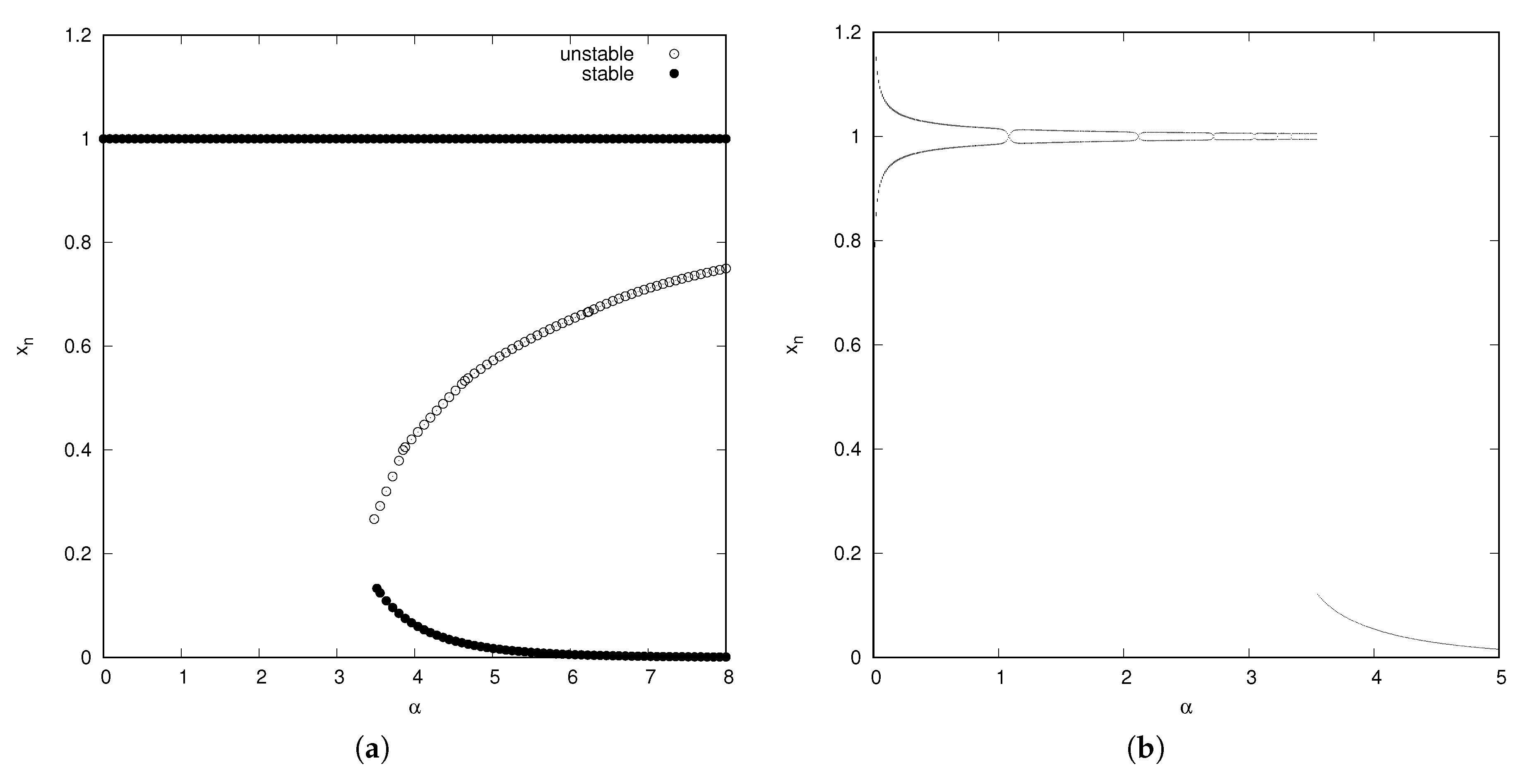
3. Analysis of the Family

Let us analyze the family of systems (Equation (2)) by classifying its equilibria along with their stability properties. The fixed points of Equation (2) satisfy the equation:

$$(\beta -1)x+(2-x)e^{-\alpha {(x-1)}^2}=0.$$

(3)

In order to focus on the intricacies of the number of roots of Equation (3) and their stability properties, we divided its analysis into three cases, namely, $\beta =1,$ which corresponds to a perturbed linear case, a basic exponential polynomial case given by $\beta =0$, and, finally, a mixed case with $\beta \in (0,1).$ Let us start with the first case.

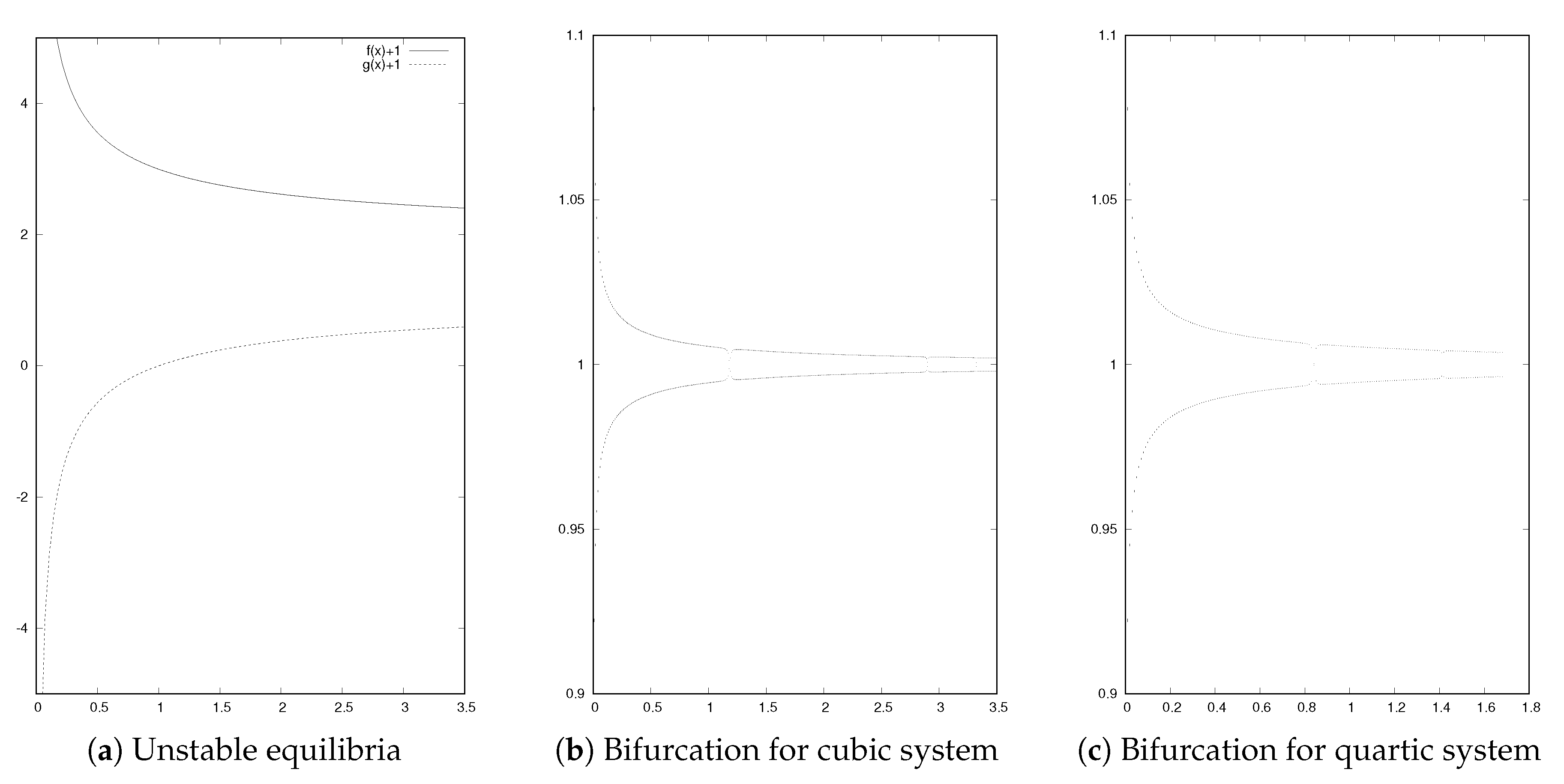
3.1. Perturbed Linear Case, $\beta =1$

This particular case allows us to analyze a more general discrete dynamical system than System (2), namely:

$$x_{n+1}=x_n+P\left(x_n\right)e^{-\alpha Q\left(x_n\right)},$$

where P and Q are polynomials. The fixed points of this new system are given by the roots of $P\left(x\right)$. Assume that Q is nonnegative and P has different roots:

$$r_0<r_1<r_2<\cdots <r_m,$$

satisfying ${\left.\frac{\left|P\right(r_j\left)\right|}{|r-r_j|}\right|}_{r=r_j}<1$ for $j=0,1,\cdots ,m.$ With these assumptions, we have the following result:

Theorem 1.

If ${(-1)}^m\frac{d^{m}P\left(x\right)}{d{x}^m}<0,$ then the system $x_{n+1}=F\left(x_n\right)=x_n+P\left(x_n\right)e^{-\alpha Q\left(x_n\right)}$ has stable fixed points at roots of P with even subindexes $x=r_j,$$j=0,2,4,\dots$ and unstable fixed points at roots of P with odd subindexes $x=r_j,$ $j=1,3,5,\dots$ for all positive values of $\alpha .$ Otherwise, the fixed points change stability, that is, roots with even (odd) subindexes are unstable (stable).

Proof. 

Notice that $F^{\prime }\left(r_j\right)=1+P^{\prime }\left(r_j\right)e^{-\alpha Q\left(r_j\right)}=1+{\left.\frac{P\left(r_j\right)}{(r-r_j)}\right|}_{r=r_j}{e}^{-\alpha Q\left(r_j\right)}.$ ☐

In particular, System (2) has only one fixed point, given by $x=2,$ for every value of $\alpha .$ That is, a branch of fixed points that is constant for every value of $\alpha$. A subregion of its basin of attraction is shown on Figure 2; notice that the system for $\alpha >3.8$ requires more iterations to converge to the fixed point for initial conditions satisfying $x_0<2$. Since $\frac{\partial f}{\partial x}(\alpha ,1,2)=1-e^{-\alpha }<1,$ the fixed point is always stable for all nonnegative values of $\alpha$, which means that the local asymptotic behavior of System (2) is trivial; its orbits converge to this fixed point or diverge to infinity. What about in practical applications, though?

In order to answer this question, we made use of bifurcation diagrams which display properties of the asymptotic solution of a dynamical system as a function of $\alpha$, allowing one to see at a glance where qualitative changes in the asymptotic solution occur. Let us observe the bifurcation diagram for System (2) with $\beta =1$ given in Figure 3a, where the initial condition is $x_0=0.05$ and the first 3000 iterations are discarded for each value of $\alpha .$ Here, the fixed point $x=2$ seems to be stable only for values of $\alpha$ in (0, 5.56). Let us observe that after the value $\alpha =5.66$, the branch of fixed points decreases down to the value of 1.982. We also obtained the same qualitative behavior when we varied the initial conditions, see Figure 3. For large $\alpha$, the fixed point is only weakly attracting. In this respect, Figure 2 seems irrelevant, but the novelty of this figure is that it shows unreal fixed points, namely, those appearing after the value $\alpha =5.66$.

How can we explain this controversial phenomenon? Here is where the fact that we are dealing with an exponential polynomial as iteration function plays a significant role, meaning that the phenomenon of slowing down takes place [30]. Notice that for $\alpha \gg 1$, the system behaves as $x_{n+1}=x_n+ϵ\left(x_n\right),$ $ϵ\left(x_n\right)$ being a small perturbation depending on $x_n$. Thus, a large number of iterations is required before transient responses have died out. Also notice that the correct asymptotic value depends on the initial condition. In Figure 3b, we show the previous behavior, but we increased the number of iterations up to 8000 and then plotted the next one hundred iterations. Clearly, the numerical asymptotic behavior is correct up to $\alpha =6.55$, whereas with 3000 iterations, it was correct only up to $\alpha =5.56.$ We carried out different simulations in order to obtain how the correct behavior depends on $\alpha$ and on initial conditions, from our results, we conclude that:

Theorem 2.

The system $x_{n+1}=x_n+(2-x_n)e^{-\alpha {(x_n-1)}^2}$ has a stable fixed point at $x=2$ for all positive values of $\alpha .$

This previous result is straightforward to verify, but, as we found out previously, in numerical calculations, the fixed point seems to vary with $\alpha .$ Therefore, special care must be taken to make sure that the orbits settle in the attracting fixed point. We have the following heuristic, which was found by bounding the number of iterations for $\alpha \in (0,8]$ by numerical means:

Remark 1.

In order to have “practical” convergence to the fixed point, that is, convergence with a tolerance of ${10}^{-7}$ for $\alpha \in (0,8]$ at least $\left[1000e^{0.3{(4+ϵ)}^2}\right]$ iterations must be performed with an initial value of $2-ϵ.$

3.2. Basic Exponential Polynomial Case, $\beta =0.$

Let us consider the basic exponential polynomial case, namely, the case when $\beta =0.$ For this case, the number of fixed points of System (2) depends on $\alpha$. For all values of $\alpha ,$ $x=1$ is a branch of fixed points. Since $\frac{\partial f}{\partial x}(\alpha ,0,1)=-1$, and computing the Schwarzian derivative of f (see References [31,32]), which is given in this case by $-\frac{{\partial }^{3}f}{\partial x^3}(\alpha ,0,1)-1.5{\left[\frac{{\partial }^{2}f}{\partial x^2}(\alpha ,0,1)\right]}^2=-6\alpha (\alpha +1)$, it follows that $x=1$ is locally stable for $\alpha >0.$ For $\alpha ⪆3.432987771$, there is another branch of fixed points which can not be obtained in an explicit analytical form. In Figure 5a, we plot the locus of fixed points that satisfy Equation (3), which consists of a horizontal line at $x=1$ and a c-shaped curve with one branch that approaches asymptotically to zero, and the other branch approaches one as $\alpha$ goes to infinity. Stability is shown with black circles and nonstability with white circles. Therefore, there are three fixed points for every value of $\alpha \ge 3.432987771$. Before we continue analyzing the fixed points of the system, we state the following two definitions from Reference [32]:

Definition 3.

Let $x_{n+1}=f(\alpha ,x_n)$ be a discrete dynamical system with a fixed point $x_f=0$ that is attracting from the left (or from the right). The point $({\alpha }_0,x_f)$ is r-slow if there exists a real number $r>1$ such that:

$$\left|f({\alpha }_0,x)-x\right|=\mathcal{O}\left(x^r\right),as x\to 0.$$

This definition is closely related to the concept of asymptotic expansions: A function $g\left(x\right)$ is asymptotic to a power series if, for fixed N and sufficiently small x:

$$g\left(x\right)-{\displaystyle \sum _{j=0}^N}{a}_j{x}^j=\mathcal{O}\left(x^{N+1}\right).$$

In our case, $g\left(x\right)=f({\alpha }_0,x),$ $N=1,$ $a_0=0$ and $a_1=1$, and we are replacing the natural number $N+1$ by a real number r. However, Definition 3 can not be used as a precise classification of slow discrete dynamical systems, since the order of a function usually only provides an upper bound on its growth rate. To avoid this inconvenience and provide a more precise classification of slowness, the following new definition is used:

Definition 4.

Let $x_{n+1}=f(\alpha ,x_n)$ be a discrete dynamical system with a r-slow point $({\alpha }_0,x_f)$. The slow point belongs to the η class of slowness if:

$$\eta =max\{r\in \mathbb{R}|({\alpha }_0,x_f\left({\alpha }_0\right))is r-slow\}.$$

In our case, the fixed point $x=1$ with arbitrary $\alpha$ is characterized as a slow fixed point belonging to the $\eta =2$ class of slowness class, meaning that its rate of convergence is similar to the oscillating system $x_{n+1}=-x_n+x_n^2.$ Thus, we expect that convergence for this system to the fixed point will require at least ${10}^5$ iterations for all initial points in the range [0, 0.99]. More concretely, as an example for a tolerance of ${10}^{-3}$ (a number relatively small), the minimum number of required iterations is 249,733 for $\alpha \in (0,1]$ with initial contition $x_0=0.5$, see Figure 4. Let us recall that for the case $\beta =1$, the required number of iterations used in the examples was in the order of ${10}^4$ iterations within a tolerance of ${10}^{-6}$.

In Figure 5b, we show a bifurcation diagram, where the lower branch of the curve is stable, whereas the upper branch is unstable. Notice that in the same figure, for $1<\alpha <3.43$, there is a transient behavior (a “ghost” solution), a behavior that will be discussed in the next section. Thus, we obtain the following theoretical result:

Theorem 3.

The system $x_{n+1}=(2-x_n)e^{-\alpha {(x_n-1)}^2}$ has a fixed point at $x=1$ for all values of $\alpha ,$ which is locally stable for $\alpha >0$. For $\alpha ⪆3.432987771$, the system has two equilibria, the larger one unstable and the smaller one stable. This last equilibrium point approaches zero as α approaches ∞.

By numerical evaluation of the orbits, we obtain (see Figure 5b):

Remark 2.

The system $x_{n+1}=(2-x_n)e^{-\alpha {(x_n-1)}^2}$ has oscillatory behavior for all initial conditions close to $x=1$ and $\alpha ⪅3.432987771.$ The oscillation consists of a 2 periodic orbit.

3.3. Mixed Case $\beta \in (0,1)$

So far, we have analyzed the two boundary values of $\beta$. For $\beta \in (0,1),$ $x=1$ is not longer a fixed point; instead, there are two branches of fixed points which are similar to those given in Figure 5a. The first branch consists of a decreasing curve that starts at the point $(0,\frac{2}{2-\beta })$ in the plane $x-\alpha$ and approaches decreasingly asymptotically to $x_f=1$ as $\alpha$ goes to infinity. The second branch is similar to the c-shaped one for the case of $\beta =0,$ meaning that for $\alpha \in [0,b(\beta \left)\right]$, there is a unique fixed point, where the values of the function $b\left(\beta \right)$ are given in Figure 6a.

Along the first branch, the equilibrium remains stable for $\alpha \in (0,\gamma (\beta \left)\right),$ where the values of function $\gamma \left(\beta \right)$ are also shown in Figure 6a. After that, the branch of equilibrium points becomes unstable, giving rise to a two periodic stable branch, which loses its stability at $b\left(\beta \right)$ for small initial conditions; for larger initial conditions, the two periodic branch bifurcates again to a fourth periodic branch and so on. For $\alpha \in \left(b\right(\beta ),\infty )$, there are three fixed points, and only the smallest one is locally stable.

Notice that the smallest fixed point approaches zero when $\alpha$ goes to infinity, making the discrete system approach a unimodal system, which means that for larger values of $\alpha ,$ the asymptotic behavior of the system is independent of initial conditions. It is important to remark that this scenario is the only case where stable periodicity is present. Moreover, the equilibria can not be shown explicitly.

Let us now vary parameter $\beta$ in search of chaotic behavior. When parameter $\beta$ is small (less than 0.26), the system basically behaves as in the previous scenario, meaning that the system is robust under such perturbation. However, as $\beta$ increases, the system behaves totally different. Such a parameter increase triggers in the system a period doubling sequence to chaos similar to the behavior of the classical logistic discrete dynamical system. This chaotic behavior is present for all values of $\beta \in ({\beta }_0,1)$, where ${\beta }_0\approx 0.26$. The values of parameter $\alpha$ where chaos is present depends on parameter $\beta$, as increasing $\beta$ also increases the values of $\alpha$ (see Figure 6b,c).

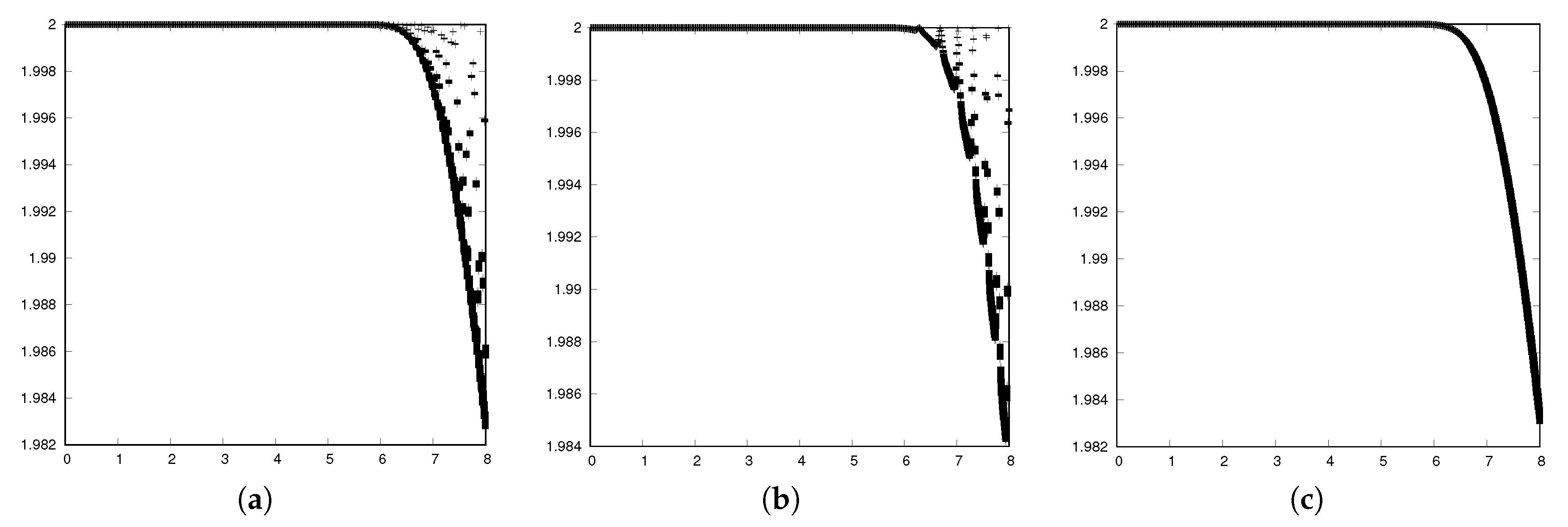
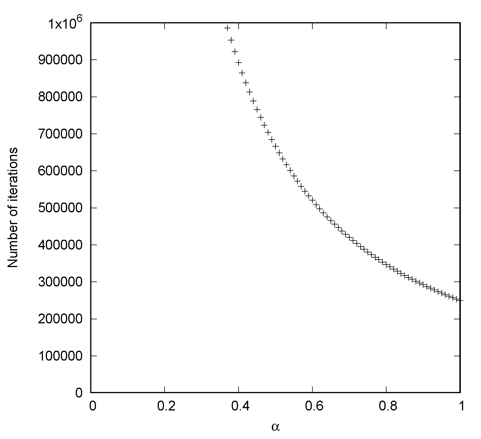
4. Transient Behavior for the Case $\mathit{\beta }=\mathbf{0}$

From now on, we will center our attention to the case when $\beta =0.$ Figure 7a is a bifurcation diagram, which is a zoom of Figure 5b, obtained by choosing the initial condition $x_0=0.3$ and plotting two hundred iterates after the first one thousand iterations have been discarded. Now, if instead of discarding the first one thousand iterations, we wait longer and discard the first five thousand iterations, we obtain the bifurcation diagram given in Figure 7b. From these two diagrams, we notice that there are some distinctive features with complicated behavior. First, the discrete system is very slow in the sense of having a slow fixed point belonging to the $\eta =2$ class of slowness class, as was defined previously. Thus, we would like to analyze the characteristic exponents associated with this system at all values of $\alpha$, especially those where we have that the “links” of the chain in the bifurcation diagrams are connected.

Let us define characteristic exponents to our system as defined by Hao [30]. Let $x_f$ be a fixed point of the system $x_{n+1}=F(\alpha ,x_n)$. Let $x_n=x_f+{ϵ}_n$ and assume that $|{ϵ}_n|$ decays as $exp(-n/\tau ),$ that is, we used the exponential function as a function of comparison. Then, we may define the time of convergence as:

$$\tau =-{\left(ln\left|\frac{\partial F}{\partial x}(\alpha ,x_f)\right|\right)}^{-1},$$

(4)

and define the critical exponent, $\Delta ,$ as the smallest power of the nonzero term in the Taylor series of $ln|\frac{\partial F}{\partial x}(\alpha ,x_f)|$ around the point $|\alpha -{\alpha }_0|,$ where ${\alpha }_0$ satisfies $|F^{\prime }({\alpha }_0,xf)|=1$. Hao discovered the exponent with value $\Delta =1$ for discrete dynamical systems. In our particular case, $ln|\frac{\partial F}{\partial x}(\alpha ,x_f)|\equiv 0.$ Therefore, the value of $\Delta$ is not even defined, which shows that our system is special and thus, it is neccesary to introduce new comparision functions in order to define a more general concept of exponent characteristics.

We already know that the behavior presented in the bifurcation diagram is not asymptotically correct, since the orbits must approach $x=1$. Thus, our goal now is to discover why such a behavior is present in the numerical simulations. Let us consider System (2) again with $\beta =0$:

$$x_{n+1}=(2-x_n)e^{-\alpha {(x_n-1)}^2}=(2-x_n){\displaystyle \sum _{k=0}^{\infty }}\frac{{(-1)}^k{\alpha }^k}{k!}{(x_n-1)}^{2k}.$$

If we truncated the previous series just to get only two terms from the series and substituting $x_n=y_n+1$, then we get the following cubic system:

$$y_{n+1}=-y_n+\alpha y_n^2(y_n-1).$$

which has zero as an equilibrium point (same as the nontruncated case) and two extra fixed points at $y=\frac{\alpha \pm \sqrt{\alpha (\alpha +8)}}{2\alpha }.$ Those are spurious equilibria for the nontruncated case. The Schwarzian derivative evaluated at zero is given by $-6\alpha (1+\alpha )$, which is negative for all nonnegative values of $\alpha$. Therefore, zero is locally stable for all $\alpha >0.$ However, the two other equilibrium points are unstable. The fact that zero is also a slow equilibrium point belonging to the $\eta =2$ class of slowness class explains why the system does not show signs of convergence to the stable equilibrium point. To give a better understanding of this slow behavior, one may compare this system to $x_{n+1}=x_{n}cos\left(\sqrt{x_n}\right)$. Both systems have the same value of slowness class. Using asymptotic analysis and telescopic cancellation, we can show that $x_n=\frac{1}{2n}+\mathcal{O}(n^{2}log\left(n\right))$, which explains the slow behavior. Notice also that the shape of the spurious equilibria corresponds to the shape of the behavior illustrated on Figure 8a. Bifurcation diagrams for the cubic system and for a quartic system are given in Figure 8b,c.

The distinctive points that simulate links (points of breakdown in the pace of convergence) correspond to eventually periodic points (see Reference [19]), and they generate a converging sequence ${\left\{{\alpha }_m\right\}}_{m=1}^{\infty }$ to the value 3.43298771..., which is the value where the second branch of fixed points arises. Each value ${\alpha }_m$ is characterized for a fixed initial condition $x_0$ by ${\alpha }_m=f^{-1}({\alpha }_{m-1},x_o)$ with ${\alpha }_1=2-x_0/(ln|2-x_0\left|\right).$ This sequence is well defined because f is a decreasing function on $\alpha$ and convergent because it is increasing and bounded. The limit is independent of initial conditions for appropriate connected sets that include the fixed point, and therefore, it inherits universal properties. Therefore, the system also shows universal properties that are characteristic of unimodal maps, and they also appear in applications with chaotic oscillations in mechanical systems.

5. Conclusions

We have discovered and established that polynomial discrete systems are complicated to analyze and most of the time, even the equilibria are impossible to express explicitly. These systems may exhibit transient behavior that does not correspond to the asymptotic behavior, a characteristic that may lead to wrong results if one is using only numerical calculations due to the impossibility of carry out an analytical process.

References

1. Arenas, A.J.; González-Parra, G.; Chen-Charpentier, B.M. A nonstandard numerical scheme of predictor– corrector type for epidemic models. Comput. Math. Appl. 2010, 59, 3740–3749. [Google Scholar] [CrossRef]
2. Kojouharov, H.V.; Dimitrov, D.T. Compatible Discretizations for Continuous Dynamical Systems. AIP Conf. Proc. 2008, 1067, 28–37. [Google Scholar]
3. Shreiber, D.I.; Barocas, V.H.; Tranquillo, R.T. Temporal variations in cell migration and traction during fibroblast-mediated gel compaction. Biophys. J. 2003, 84, 4102–4114. [Google Scholar] [CrossRef]
4. Zaliapin, I.; Semenova, I.; Kashina, A.; Rodionov, V. Multiscale trend analysis of microtubule transport in melanophores. Biophys. J. 2005, 88, 4008–4016. [Google Scholar] [CrossRef] [PubMed]
5. Simson, R.; Sheets, E.D.; Jacobson, K. Detection of temporary lateral confinement of membrane proteins using single-particle tracking analysis. Biophys. J. 1995, 69, 989–993. [Google Scholar] [CrossRef] [Green Version]
6. Fujiwara, T.; Ritchie, K.; Murakoshi, H.; Jacobson, K.; Kusumi, A. Phospholipids undergo hop diffusion in compartmentalized cell membrane. J. Cell Biol. 2002, 157, 1071–1081. [Google Scholar] [CrossRef]
7. Fiutak, J.; Mizerski, J.Z. Transient behaviour of laser. Phys. B 1980, 39, 347–352. [Google Scholar] [CrossRef]
8. Tang, C.; Telle, J.; Ghizoni, C. Transient effects in wavelength-modulated dye lasers. Appl. Phys. Lett. 1975, 26, 534–537. [Google Scholar] [CrossRef]
9. Krapivsky, P.L.; Redner, S.; Ben-Naim, E. A Kinetic View of Statistical Physics; Cambridge University Press: Cambridge, UK, 2010. [Google Scholar]
10. Castellano, C.; Fortunato, S.; Loreto, V. Statistical physics of social dynamics. Rev. Mod. Phys. 2009, 81, 591. [Google Scholar] [CrossRef]
11. Chowdhury, D.; Santen, L.; Schadschneider, A. Statistical Physics of Vehicular Traffic and Some Related Systems. Phys. Rep. 2000, 329, 199–329. [Google Scholar] [CrossRef]
12. Hinton, E. The dynamic transient analysis of axisymmetric circular plates by finite element method. J. Sound Vib. 1976, 46, 465–472. [Google Scholar] [CrossRef]
13. Kunow-Baumhauer, A. The response of a beam subjected to a transient pressure wave load. J. Sound Vib. 1984, 92, 491–506. [Google Scholar] [CrossRef]
14. Hastings, A. Transients: The key to long-term ecological understanding? Trends. Ecol. Evol. 2004, 19, 39–45. [Google Scholar] [CrossRef] [PubMed]
15. Van Geest, G.; Coops, H.; Scheffer, M.; van Nes, E. Long Transients Near the Ghost of a Stable State in Eutrophic Shallow Lakes with Fluctuating Water Levels. Ecosystems 2007, 10, 37–47. [Google Scholar] [CrossRef] [Green Version]
16. Schaffer, W.M.; Kendall, B.; Tidd, C.W.; Olsen, L.F. Transient periodicity and episodic predictability in biological dynamics. IMA J. Math. Appl. Med. Biol. 1993, 10, 227–247. [Google Scholar] [CrossRef]
17. Fisher, R.S.; Boas, W.E.; Blume, W.; Elger, C.; Genton, P.; Lee, P.; Engel, J. Epileptic Seizures and Epilepsy: Definitions Proposed by the International League Against Epilepsy (ILAE) and the International Bureau for Epilepsy (IBE). Epilepsia 2005, 46, 470–472. [Google Scholar] [CrossRef] [Green Version]
18. Grüne, L.; Stieler, M. Asymptotic stability and transient optimality of economic MPC without terminal conditions. J. Process Control 2014, 24, 1187–1196. [Google Scholar] [CrossRef] [Green Version]
19. Solis, F.; Jódar, L. Nonisolated slow convergence in discrete dynamical systems. Appl. Math. Lett. 2004, 17, 597–599. [Google Scholar] [CrossRef] [Green Version]
20. Solis, F.; Felipe, R. Slow convergence of Maps. Nonlinear Stud. 2001, 8, 389–392. [Google Scholar]
21. Weidner, P. The Durand-Kerner method for trigonometric and exponential polynomials. Computing 1988, 40, 175–179. [Google Scholar] [CrossRef]
22. Schock, E. Approximate solution of ill-posed equations: Arbitrarily slow convergence vs. superconvergence. In Constructive Methods for the Practical Treatment of Integral Equations; Birkhäuser: Basel, Switzerland, 1985; pp. 234–243. [Google Scholar]
23. Braun, M. Differential Equations and Their Applications: An Introduction to Applied Mathematics; Springer: New York, NY, USA, 2013; Volume 15. [Google Scholar]
24. Dunham, C.B. Chebyshev approximation by exponential-polynomial sums. J. Comput. Appl. Math. 1979, 5, 53–57. [Google Scholar] [CrossRef] [Green Version]
25. Viswanathan, K.S. Statistical mechanics of a one-dimensional lattice gas with exponential-polynomial interactions. Comm. Math. Phys. 1976, 47, 131–141. [Google Scholar] [CrossRef]
26. Boyadzhiev, K.N. Exponential Polynomials, Stirling Numbers, and Evaluation of Some Gamma Integrals. Abstr. Appl. Anal. 2009, 2009, 168672. [Google Scholar] [CrossRef]
27. Mayoral, E.; Robledo, A. Multifractality and nonextensivity at the edge of chaos of unimodal maps. Phys. A 2004, 340, 219–226. [Google Scholar] [CrossRef] [Green Version]
28. Andrecut, M.; Ali, M.K. Robust chaos in smooth unimodal maps. Phys. Rev. E 2001, 64, 025203–025205. [Google Scholar] [CrossRef] [PubMed]
29. Jensen, R.V.; Ma, L.K.H. Nonuniversal behavior of asymmetric unimodal maps. Phys. Rev. A 1985, 31, 3993–3995. [Google Scholar] [CrossRef]
30. Hao, B.L. Universal Slowing-Down Exponent Near Periodic-Doubling Bifurcation Points. Phys. Lett. A 1981, 86, 267–268. [Google Scholar] [CrossRef]
31. San Martín, J.; Porter, M.A. Convergence Time towards Periodic Orbits in Discrete Dynamical Systems. PLoS ONE 2014, 9, e92652. [Google Scholar] [CrossRef] [PubMed] [Green Version]
32. Solis, F.; Chen, B.; Kojouharov, H. A classification of slow convergence near parametric periodic points of discrete dynamical systems. Int. J. Comput. Math. 2016, 93, 1011–1021. [Google Scholar] [CrossRef]
Figure 1. Graphs of the iteration function f ( α , β , x ) with α = 4 and with different values of β .
Mca 24 00013 g001
Figure 2. Basin of attraction of the fixed point x = 2 for α ( 0 , 7 ) and initial conditions x 0 [ 1.5 , 2.2 ] . Colors denotes the number of iterations within a tolerance of 10 3 .
Mca 24 00013 g002
Figure 3. Bifurcation diagram of System (2) with initial conditions (a) 0.05, (b) 0.19, (c) 1.7. Horizontal axis is α and vertical axis is x n . n > 3000 for (a) and n > 8000 for (b,c).
Mca 24 00013 g003
Figure 4. Number of iterations required to obtain convergence to the fixed point given a tolerance of 10 3 for α ( 0 , 1 ) and initial condition x 0 = 0.5 .
Mca 24 00013 g004
Figure 5. (a) Fixed points for System (2) when β = 0 . (b) Bifurcation diagram with initial condition x 0 = 0.3 and 1000 initial iterations discarded.
Mca 24 00013 g005
Figure 6. (a) Graph of b ( β ) . (b) Bifurcation diagram for β = 0.3 . (c) Bifurcation diagram for β = 0.6 .
Mca 24 00013 g006
Figure 7. Bifurcation diagrams for β = 0 and initial condition x 0 = 0.3 . Horizontal axis is α and vertical axis is x n . (a) First 1000 iterations discarded. (b) First 5000 iterations discarded. (c) Both diagrams (a) and (b).
Mca 24 00013 g007
Figure 8. Bifurcation diagrams for β = 0 and initial condition x 0 = 0.3 . Horizontal axis is α and vertical axis is x n .
Mca 24 00013 g008