Minimizing an Insurer’s Ultimate Ruin Probability by Reinsurance and Investments

Abstract

In this paper, we work with a diffusion-perturbed risk model comprising a surplus generating process and an investment return process. The investment return process is of standard a Black–Scholes type, that is, it comprises a single risk-free asset that earns interest at a constant rate and a single risky asset whose price process is modelled by a geometric Brownian motion. Additionally, the company is allowed to purchase noncheap proportional reinsurance priced via the expected value principle. Using the Hamilton–Jacobi–Bellman (HJB) approach, we derive a second-order Volterra integrodifferential equation which we transform into a linear Volterra integral equation of the second kind. We proceed to solve this integral equation numerically using the block-by-block method for the optimal reinsurance retention level that minimizes the ultimate ruin probability. The numerical results based on light- and heavy-tailed individual claim amount distributions show that proportional reinsurance and investments play a vital role in enhancing the survival of insurance companies. But the ruin probability exhibits sensitivity to the volatility of the stock price.

1. Introduction

The problem of minimizing the ruin probability, when the insurance company is allowed to invest part of its surplus in the money and stock markets and to reduce its risk by entering into proportional reinsurance treaties, has been extensively studied in different forms since the ground-breaking work of Bachelier [1]. Liang and Guo [2] found that the minimal ruin probability maximizes the adjustment coefficient $\gamma$ under proportional reinsurance and that it satisfies the Lundberg inequality $\psi \left(u\right)\le {\mathrm{e}}^{-\gamma u}$. Wang [3] considered the case of multiple risky assets in an optimal investment problem for an insurer whose surplus evolves according to a jump-diffusion process, while Liang and Guo [4] considered the optimal reinsurance problem by combining quota-share and excess-of-loss reinsurance. The authors derived explicit expressions for the value function and the optimal strategies.

Kasozi et al. [5] studied the problem of controlling ultimate ruin probability by quota-share reinsurance arrangements for an insurer that is allowed to invest part of the surplus in a risk-free and risky asset. They found that, for selected parameter values, the optimal quota-share retention lies in the interval $(0.2,0.4)$, i.e., the company should cede between 60% and $80\%$ of its risks to a reinsurer. This study also found that the ruin probabilities increase when stock prices become more volatile. However, while [5] assumed cheap reinsurance, in this paper we use noncheap reinsurance. Zhou et al. [6] investigated the optimal proportional reinsurance and investment problem for a jump-diffusion surplus process in a constant elasticity of variance (CEV) stock market.

Liu and Yang [7] revisited the model in Hipp and Plum [8] by incorporating a risk-free interest rate. Since they could not obtain closed-form solutions in this case, they provided numerical results for optimal strategies for maximizing the survival probability under different claim-size distribution assumptions. Schmidli [9] proved the existence and uniqueness of a solution of the ruin probability minimization problem in a model compounded by investment and dynamic proportional reinsurance for the case $\lambda >0$ and $\sigma =0$, i.e., when there is no diffusion and when F has a bounded density. But while [9] uses proportional reinsurance in minimizing ruin probabilities in the Cramér–Lundberg model, this paper considers proportional reinsurance and investments of Black–Scholes type in the diffusion-perturbed model.

With the objective of determining the optimal investment and reinsurance strategies, Liang and Young [10] studied the problem of minimizing the probability of ruin in the presence of per-loss reinsurance for an insurance company whose risk process follows a compound Poisson process or its diffusion approximation. Assuming that the financial market in which the company invests follows the Black–Scholes model, and under minimal assumptions regarding admissible reinsurance forms, ref. [10] showed that the optimal per-loss reinsurance policy is excess-of-loss reinsurance. They found that for cheap reinsurance under both models, full reinsurance is never optimal, a result consistent with Mossin [11]. While under the compound Poisson model it is optimal not to buy reinsurance when the surplus is sufficiently low, for the diffusion approximation model the insurer always buys some amount of reinsurance but the optimal retention is inversely proportional to the surplus. This is also true of the optimal investment level as it decreases with an increase in the surplus. However, ref. [10] concerned itself with excess-of-loss reinsurance while this paper explores optimality of noncheap proportional reinsurance and employs different numerical methods from those of [10].

Zhu et al. [12] studied the optimal proportional reinsurance and investment problem in a general jump-diffusion financial market. With the objective of maximizing the expected exponential utility of terminal wealth, they added a general jump to the price of the risky asset, so that the financial market follows a general jump-diffusion model. They also incorporated a reasonable constraint on the proportional reinsurance strategy, thus making the model more reasonable and realistic, and derived closed-form expressions for the value function and optimal strategy. Glineur and Walhin [13] revisited de Finetti’s retention problem for proportional reinsurance by applying the convex optimization method. The authors extended the result to variable quota-share and surplus reinsurance with table of lines and showed, by means of a numerical example, that neither variable quota share reinsurance nor surplus reinsurance with table of lines may be considered as optimal reinsurance structures. They were able to determine the optimal quota-share and surplus reinsurance strategies. However, the numerical example also led them to the conclusion that there exists no general rule asserting superiority of either quota-share-type or surplus-type reinsurance above the other.

An insurance company is said to have experienced ruin when its surplus becomes negative, thus making it impossible for the company to meet its financial obligations (e.g., claims). The time of ruin is the first time that the cedent’s surplus process enters $(-\infty ,0)$ and the associated probability is referred to as the ultimate ruin probability. Ruin is a technical term which does not necessarily mean that the company is bankrupt, but rather that bankruptcy is at hand and that the company should therefore be prompted to take action to improve its solvency status. Thus, insurance companies customarily take precautions to avoid ruin. These precautions are referred to as control variables and include investments, capital injections or refinancing, portfolio selection, volume control through the setting of premiums and reinsurance arrangements, to mention but a few. This study focuses on reinsurance as a risk control mechanism for a company that also invests part of its surplus in risk-free and risky assets.

According to Jang and Kim [14], insurance companies generally face two sources of risk, viz., an insolvency risk that arises from unexpectedly large insurance claims, and a market risk that arises from risky investments in financial markets. Reinsurance can help mitigate the insolvency risk, while investing in some risk-free assets such as short-term bonds and money market funds could reduce the market risk. Reinsurance is the transfer of risk from a direct insurer (the cedent) to a second insurance carrier (the reinsurer). It serves the purpose of offering protection to cedents against very large individual claims or fluctuations in their aggregate portfolio of risks, as well as diversifying the financial losses caused by it. Reinsurance therefore allows the cedent to pass on some of its risk to the reinsurer but at the expense of a portion of the aggregate premiums receivable from the policyholders [15].

Mikosch [16] has pointed out that reinsurance treaties are of two types; random walk type reinsurance which includes proportional, excess-of-loss and stop-loss reinsurance, and extreme value type reinsurance which includes the largest claims and ECOMOR reinsurance (excédent du coût moyen relatif or ‘excess of the average cost’). Proportional, or pro rata, reinsurance is a common form of reinsurance for claims of ‘moderate’ size, and requires the reinsurer to cover a fraction of each claim equal to the fraction of total premiums ceded to the reinsurer. Proportional reinsurance treaties are traditionally subdivided into two forms; quota-share and surplus reinsurance. Quota-share reinsurance is a common type of proportional reinsurance in which the cedent and the reinsurer agree to share claims and premiums in the same proportion which remains constant throughout the portfolio [17]. With surplus reinsurance the reinsurer agrees to accept an individual risk with sum insured in excess of the direct retention limit set by the cedent [18].

It has been noted in [19] that proportional reinsurance is the easiest way of covering an insurance portfolio. This paper focuses on quota-share (QS) proportional reinsurance due to its simplicity, but other forms of reinsurance could also be used. In addition, the reinsurer pays a ‘ceding commission’ to the cedent to compensate for the costs of underwriting the ceded business. This commission is ignored in this study. Thus, if a cedent enters into a quota-share reinsurance treaty with a reinsurer, then they will share claims and premiums according to a retention level $k\in [0,1]$. For every claim X that occurs at the time where the surplus prior to the claim payment is u, the cedent pays $kX$ while the reinsurer pays $(1-k)X$. Similarly, for every premium amount c received by the insurer, $c^R=(1-k)c$ is paid to the reinsurer and $c^k=c-c^R$ is retained by the cedent. Since the factor $(1-k)$ represents the proportion of claims or premiums ceded to the reinsurer, it is called the cession level. It should be noted that for cheap reinsurance $c^k=kc$.

It has been argued in the literature that the Cramér–Lundberg model is somewhat inadequate for modelling real-world insurance processes (see, e.g., [20,21]). The limitations of this model quickly led to its generalizations (e.g., in [22,23,24]), even at the cost of tractability. The more complex the model gets, the more difficult its analysis and the drawing of conclusions becomes. In this paper, we make generalizations to the well known Cramér–Lundberg model by adding a diffusion term and also allowing the company to invest in the financial markets with returns of a Black–Scholes type. Thus, this paper focuses on ultimate ruin and considers proportional reinsurance coupled with investments as mechanisms for reducing the insurer’s ultimate ruin probability. Reinsurance can protect insurers against potentially large losses, while investment of insurance premiums enables insurers to achieve certain management objectives, some of the most common of which are the minimization of the ruin probability, maximization of expected utility and mean-variance criteria. Li et al. [25] have pointed out that insurance companies commonly employ integrated reinsurance and investment strategies to increase their underwriting capacity, stabilize underwriting results, protect themselves against catastrophic losses, and achieve financial growth.

The models studied in this paper result in Volterra integral equations of the second kind (VIE-2s). As Press et al. [26] have pointed out, there is general consensus that the block-by-block method, first proposed by Young [27], is the best of the higher order methods for solving VIE-2s. The block-by-block methods are essentially extrapolation procedures which produce a block of values at a time. They are advantageous over linear multistep and step-by-step methods in that they can be of higher order and still be self-starting. Apart from not requiring special starting procedures or values, block-by-block methods have a simple structure, allow for easy switching of step-size and have the ability to compute several values of the unknown function at the same time [28,29]. In addition, the block-by-block method is chosen in this paper over such methods as saddlepoint approximation, importance sampling simulation, upper and lower bounds, Fast-Fourier Transform (FFT) and diagonally implicit multistep block [30,31,32] because it is a fourth-order method while most of the other methods are of order less than four. In fact, some of the methods mentioned above are used for directly computing ruin probabilities and not for solving integrodifferential or integral equations.

Other methods have been used to solve integrodifferential equations arising in engineering such as the local Galerkin integral equation and thin plate spline collocation methods for solving second-order Volterra integrodifferential equations (VIDEs) with time-periodic coefficients [33,34]. Both of these methods are meshless and therefore do not require any background interpolation. As for the collocation method proposed by Cardone et al. [35], although it has the advantages of variable step-size implementation, high order of convergence, strong stability and a high degree of flexibility, it suffers from the order-reduction phenomenon when applied to stiff problems since it does not have a uniform order of convergence.

In the literature, two-, three- and four-block block-by-block methods have been used to solve Volterra integral equations (e.g., [36] for non-linear VIE-2s, [37] for a system of linear VIE-2s). More recently, Kasozi and Paulsen [38] used the two-block block-by-block method to study the flow of dividends under a constant interest force. They derived a linear VIE-2 and applied a fourth-order block by-block method of Paulsen et al. [39] in conjunction with Simpson’s rule to solve the Volterra integral equation for the optimal dividend barrier. In another study, Kasozi and Paulsen [40] applied a fourth-order block-by-block method to the numerical solution of the Volterra integral equation (VIE) for ultimate ruin in the Cramér–Lundberg model compounded by a constant force of interest. More pertinent literature on the block-by-block method is available, for example, in [41,42].

The remainder of the paper is organized as follows. In Section 2, we present the models to be studied and the underlying assumptions. In Section 3, we give the Hamilton–Jacobi–Bellman (HJB) equation and verification theorems for the ruin probabilities under proportional reinsurance, as well as the corresponding Volterra integrodifferential and integral equations. Section 4 contains a presentation of numerical results and examples based on light- and heavy-tailed individual claim-size distributions. Finally, in Section 5 we give some concluding remarks and possible extensions to this work.

2. The Models

To give a rigorous mathematical formulation of the problem, we assumed that all stochastic quantities are defined on a complete filtered probability space $(\mathsf{\Omega },\mathcal{F},$ ${\left\{{\mathcal{F}}_t\right\}}_{t\in {\mathbb{R}}^{+}},\mathbb{P})$ satisfying the usual conditions, i.e., the filtration ${\left\{{\mathcal{F}}_t\right\}}_{t\in {\mathbb{R}}^{+}}$, which represents the information available at time t and forms the basis for all decision-making, is right-continuous and $\mathbb{P}$-complete. Right-continuity is necessary for ensuring that the ruin time defined later in this section is a stopping time. The risk process considered in this paper is made up of two important processes; the insurance process and the investment-generating process. In the absence of reinsurance, the insurance process ${\left\{P_t\right\}}_{t\in {\mathbb{R}}^{+}}$ is given by the diffusion-perturbed model

$$P_t=ct+{\sigma }_1{W}_{1,t}-S_t,t\ge 0,$$

(1)

where the process $S_t$, defined as

$$S_t=\left\{\begin{array}{cc}{\sum }_{i=1}^{N_t}{X}_i\hfill & \mathrm{if} N_t>0\hfill \\ 0\hfill & \mathrm{if} N_t=0\hfill \end{array}\right.,$$

is a compound Poisson process representing the aggregate claims made by policyholders. Here, the premiums are assumed to be calculated according to the expected value premium principle and to be collected continuously over time at a constant rate $c=(1+\eta )\lambda \mu >0$, where $\eta >0$ is the relative safety loading of the insurer. $W_1$ is a one-dimensional standard Brownian motion independent of the compound Poisson process $S_t$, $\left\{N_t\right\}$ is a homogeneous Poisson process with constant intensity $\lambda$ and the claim sizes ${\left\{X_i\right\}}_{i\in \mathbb{N}}$ are a sequence of strictly positive i.i.d. random variables. We assumed that the processes ${\left\{X_i\right\}}_{i\in \mathbb{N}}$, ${\left\{N_t\right\}}_{t\in {\mathbb{R}}^{+}}$ and ${\left\{W_{1,t}\right\}}_{t\in {\mathbb{R}}^{+}}$ were mutually independent. We denoted by F the distribution function of $X_i$, by $\mu =\mathbb{E}\left[X_i\right]$ its first moment and by $M_X\left(t\right)=\mathbb{E}\left[e^{t{X}_i}\right]$ its moment-generating function. We assumed that $F\left(0\right)=0$ and that at least one of ${\sigma }_1$ or $\lambda$ was non-zero.

The diffusion term ${\sigma }_1{W}_1$ in the basic model (1) has been interpreted in a two-fold manner in the literature. On the one hand, ${\sigma }_1{W}_1$ could be understood as standing for the uncertainty or random fluctuations associated with the insurance process at time t (the U-S case). This means that the aggregate claims up to time t are given by the compound Poisson process $S_t$. This is the interpretation assumed in this paper. On the other hand, ${\sigma }_1{W}_1$ could represent the additional small claims which account for uncertainty associated with the insurance market or the economic environment (the A-C case), so that the aggregate claims process is $S_t-{\sigma }_1{W}_{1,t}$ (see, e.g., [6]). It should be noted that, given an initial surplus u, when there is no volatility in the surplus and claim amounts (i.e., when ${\sigma }_1=0$), Equation (1) becomes the well-known classical risk process (or the Cramér–Lundberg model).

Given that the insurer controls its insurance risk by taking QS proportional reinsurance at a retention level $k\in [0,1]$, the insurance process in the presence of QS reinsurance is now

$$P_t^k=c^{k}t+k{\sigma }_1{W}_{1,t}-k{S}_t$$

(2)

with dynamics

$$d{P}_t^k=c^{k}dt+k{\sigma }_{1}d{W}_{1,t}-kd{S}_t.$$

(3)

If $k=0$ then there is full reinsurance, i.e., the entire portfolio of risks is ceded to the reinsurer, whereas if $k=1$ then there is no reinsurance. The case $k=1$ is precisely the model considered in [39,43]. In this study, we assumed noncheap reinsurance, meaning that the reinsurer used a higher safety loading than the insurer. Otherwise, the insurance company can take full reinsurance and receive a positive return without any risk, which is undesirable from the reinsurer’s standpoint, as was demonstrated in [44]. Thus, if $c^R=(1-k)(1+\theta )\lambda \mu$ is the reinsurance premium to be paid for the QS reinsurance, then the insurance premium rate is $c^k=c-c^R=[k(1+\theta )-(\theta -\eta )]\lambda \mu$, where $\theta \in (\eta ,\infty )$ is the reinsurer’s safety loading. In order for the net profit condition (NPC) to be fulfilled, that is,

$$\left[k\right(1+\theta )-(\theta -\eta \left)\right]\lambda \mu -k\lambda \mu >0,$$

we need

$$\begin{array}{c}\hfill k>\underline{k}=1-\frac{\eta }{\theta },\end{array}$$

(4)

otherwise ruin is certain for any initial capital $u>0$. Note that in noncheap reinsurance the fraction of the premiums diverted to the reinsurer is larger than that of each claim covered by the reinsurer. The classical risk process with noncheap reinsurance was also studied by, among others, Ma et al. [45] who obtained the minimal probability of ruin as well as the optimal proportional reinsurance strategy using the dynamic programming approach, while cheap reinsurance (i.e., $\theta =\eta$) was considered in Schmidli [46] who allowed for investment in a risky asset and obtained, by means of an HJB equation, the optimal reinsurance and investment strategies for minimizing the ultimate ruin probability.

Suppose the insurer invests part of its surplus, into say, a risk-free asset (a bond) and a risky asset (stocks) as in [7]. Let the return on investments process be:

$$R_t=rt+{\sigma }_2{W}_{2,t},t\ge 0,R_0=0,$$

(5)

where r is the risk-free interest rate, so that $R_t=rt$ implies that one unit invested now will be worth $e^{rt}$ at time t; $W_2$ is another one-dimensional Brownian motion independent of the surplus-generating process P and ${\sigma }_2$ is the volatility of the stock price, so that the diffusion term ${\sigma }_2{W}_2$ accounts for random fluctuations in the investment returns. Equation (5) is actually the famous Black–Scholes option pricing formula according to which the price of a stock is assumed to follow the stochastic differential equation

$$Y_t=Y_0+{\int }_0^t{Y}_{s}d{R}_s,$$

(6)

where $Y_0$ is the stock price at $t=0.$ The process Y is a geometric Brownian motion. The solution to (6) is the value of the stock at time t and is given by $Y_t=Y_{0}exp\{(r-\frac{1}{2}{\sigma }_2^2)t+{\sigma }_2{W}_{2,t}\}$.

The risk process is therefore made up of a combination of the surplus-generating process compounded by proportional reinsurance (2) and the investment-generating process (5). Thus, the insurance portfolio is represented by the risk process $U^k={\left\{U_t^k\right\}}_{t\in {\mathbb{R}}^{+}}$ which has dynamics

$$d{U}_t^k=d{P}_t^k+U_{t^{-}}^{k}d{R}_t.$$

(7)

A reinsurance strategy k is said to be admissible if it is ${\mathcal{F}}_t$-progressively measurable and takes values from the set $[0,1]$. Thus, given an admissible reinsurance strategy $k\in [0,1]$, and assuming that the mutually independent processes P and R belong to the rather general class of semimartingales, then under some weak additional assumptions the risk process $U^k$ is mathematically the solution of the linear stochastic differential equation (SDE)

$$U_t^k=u+P_t^k+{\int }_0^t{U}_{s^{-}}^{k}d{R}_s,$$

(8)

where $U_0^k=u>0$ is the initial surplus of the insurance company, $P_t^k$ is the basic insurance (or surplus-generating) process in Equation (2), $R_t$ the investment-generating process in Equation (5) and $U_{t^{-}}^k$ denotes the insurer’s surplus (incorporating both proportional reinsurance and investments) just prior to time t. Paulsen [47], gave the solution of (8) as

$$U_t^k={\overline{R}}_t\left(u+{\int }_0^t{\overline{R}}_s^{-1}d{P}_s^k\right),$$

(9)

where

$${\overline{R}}_t=exp\left\{\left(r-\frac{1}{2}{\sigma }_2^2\right)t+{\sigma }_2{W}_{2,t}\right\},t\ge 0$$

is the geometric Brownian motion so extensively used in mathematical finance and is the solution of the SDE $d{\overline{R}}_t\stackrel{It\widehat{o}}{=}r{\overline{R}}_{t}dt+{\sigma }_2{\overline{R}}_{t}d{W}_{2,t}$, with ${\overline{R}}_0=1$.

Since both P and R have stationary independent increments, $U_t$ is a homogeneous strong Markov process. We defined the value function of this optimization problem as

$$\begin{array}{c}\hfill {\psi }^k\left(u\right)=\mathbb{P}(U_t^k\le 0\mathrm{for}\mathrm{some}t\ge 0|U_0^k=u)=\mathbb{P}({\tau }^k<\infty |U_0^k=u),\end{array}$$

where ${\psi }^k\left(u\right)$ is the ultimate ruin probability under the reinsurance policy k when the initial surplus is u and ${\tau }^k=inf\{t>0|U_t^k<0\}$ is the time of ruin, with ${\tau }^k=\infty$ if $U_t^k$ remains positive. Then the objective is to find the optimal value function, i.e., the minimal ruin probability

$$\begin{array}{c}\hfill \psi \left(u\right)=\underset{k\in [0,1]}{inf}{\psi }^k\left(u\right)\end{array}$$

(10)

and the optimal policy $k^{*}$ such that ${\psi }^{k^{*}}\left(u\right)=\psi \left(u\right)$, considered optimal if $k^{*}$ minimizes the ruin probability. Since the ultimate survival probability ${\varphi }^k\left(u\right)=\mathbb{P}({\tau }^k=\infty |U_0^k=u)=1-{\psi }^k\left(u\right)$, we may alternatively find the value of $k^{*}$ which maximizes $\varphi \left(u\right)$, so that the optimal value function becomes

$$\begin{array}{c}\hfill \varphi \left(u\right)=\underset{k\in [0,1]}{sup}{\varphi }^k\left(u\right).\end{array}$$

(11)

3. HJB, Integrodifferential and Integral Equations

In this section, we derived the HJB equation for the problem and the corresponding integrodifferential and integral equations. By Itô’s formula, the infinitesimal generator of the process $U_t^k$ in Equation (8) is given by the integrodifferential operator

$$\begin{array}{c}\hfill \mathcal{A}g\left(u\right)=\frac{1}{2}\left({\sigma }_2^2{u}^2+k^2{\sigma }_1^2\right)g^{″}\left(u\right)+(ru+c^k)g^{\prime }\left(u\right)+\lambda {\int }_0^{\infty }\left(g(u-kx)-g\left(u\right)\right)dF\left(x\right).\end{array}$$

(12)

Since the investment-generating process $R_t$ is governed by (5), it follows that under weak assumptions the ruin probability $\psi \left(u\right)$ is twice continuously differentiable on $(0,\infty )$ and is a solution to the equation (see [48])

$$\mathcal{A}\psi \left(u\right)=-\lambda \overline{F}\left(u\right),$$

(13)

where $\overline{F}\left(u\right)=1-F\left(u\right)$, with boundary conditions ${lim}_{u\to \infty }\psi \left(u\right)=0$ and $\psi \left(u\right)=1$ if ${\sigma }_1>0$ (see Theorem 1 below). Sometimes it is more convenient, as we did in this paper, to work with the survival probability $\varphi \left(u\right)=1-\psi \left(u\right)$, in which case (13) becomes

$$\mathcal{A}\varphi \left(u\right)=0.$$

The integrodifferential operator (12) does not easily give rise to closed-form solutions, hence the need for the use of numerical methods. The following theorem is proved in [48].

Theorem 1.

Let ${\tau }^k=inf\{t>0|U_t^k<0\}$ be the ruin time, with ${\tau }^k=\infty$ if $U_t^k\ge 0\forall t$. Assume that the equation $\mathcal{A}\varphi \left(u\right)=0$ has a bounded, twice continuously differentiable solution (once continuously differentiable if ${\sigma }_1={\sigma }_2=0$) that satisfies the boundary conditions

$$\begin{array}{c}\hfill \varphi \left(u\right)=0\mathrm{on}u<0,\\ \hfill \varphi \left(0\right)=0\mathrm{if}{\sigma }_1^2>0,\\ \hfill \underset{u\to \infty }{lim}\varphi \left(u\right)=1.\end{array}$$

(14)

Then $\varphi \left(u\right)=1-\psi \left(u\right)$ is the survival probability.

We now present the HJB equation for this optimization problem.

Theorem 2.

Assume that the survival probability $\varphi \left(u\right)$ defined by (11) is twice continuously differentiable on $(0,\infty )$. Then, for $u>0$, $\varphi \left(u\right)$ satisfies the HJB equation

$$\begin{array}{c}\hfill \underset{k\in [0,1]}{sup}\left\{\mathcal{A}\varphi \left(u\right)\right\}=0,\end{array}$$

(15)

where $\mathcal{A}$ is the infinitesimal generator (12) of the process $U_t^k$.

Proof. 

See [49]. ☐

The function $\varphi \left(u\right)$ will satisfy the HJB Equation (15) only if it is strictly increasing, strictly concave, twice continuously differentiable and satisfies $\varphi \left(u\right)\to 1$ for $u\to \infty$[8]. In the following, therefore, $\varphi \left(u\right)$ will be assumed to be strictly increasing. This is consistent with the smoothness assumption and the intuition that the more wealth there is (through investment), the higher the probability of survival of the insurance company. It will also be assumed that $\varphi \left(u\right)$ is concave. To ensure smoothness and concavity, the claim density function must be locally-bounded [7].

The following verification theorem, whose proof is similar to that of Theorem 2 in Kasumo et al. [44], is essential for solving the associated control problem as it leads to the integrodifferential equation for the problem.

Theorem 3.

Suppose $\mathsf{\Phi }\in C^2$ is an increasing strictly concave function satisfying the HJB Equation (15) subject to the boundary conditions

$$\begin{array}{c}\hfill \mathsf{\Phi }\left(u\right)=0\mathrm{on}u<0\\ \hfill \mathsf{\Phi }\left(0\right)=0\mathrm{if}{\sigma }^2>0\\ \hfill \underset{u\to \infty }{lim}\mathsf{\Phi }\left(u\right)=1\end{array}$$

for $0<u\le \infty$. Then the maximal survival probability $\varphi \left(u\right)$ given by (11) coincides with Φ. Furthermore, if $k^{*}$ satisfies

$$\frac{1}{2}\left({\sigma }_2^2{u}^2+{k^{*}}^2{\sigma }_1^2\right){\mathsf{\Phi }}^{{}^{″}}\left(u\right)+(ru+c^{k^{*}}){\mathsf{\Phi }}^{{}^{\prime }}\left(u\right)+\lambda \left[{\int }_0^u\mathsf{\Phi }\left(u-k^{*}x\right)dF\left(x\right)-\mathsf{\Phi }\left(u\right)\right]=0$$

(16)

when $0\le u<\infty$, where $c^{k^{*}}=[k^{*}(1+\theta )-(\theta -\eta )]\lambda \mu$, then the policy $k^{*}$ is an optimal policy, that is, $\mathsf{\Phi }\left(u\right)=\varphi \left(u\right)={\varphi }^{k^{*}}\left(u\right)$.

The integrodifferential equation for the survival probability $\varphi \left(u\right)$, which follows immediately from Theorem 3, is of the form $\mathcal{A}\varphi \left(u\right)=0$ (since, by Equation (14), $\varphi \left(u\right)=0$ for $u<0$), where $\mathcal{A}$ is the infinitesimal generator (12) of the underlying risk process, that is,

$$\frac{1}{2}\left({\sigma }_2^2{u}^2+k^2{\sigma }_1^2\right){\varphi }^{{}^{″}}\left(u\right)+(ru+c^k){\varphi }^{{}^{\prime }}\left(u\right)+\lambda {\int }_0^u\varphi (u-kx)dF\left(x\right)-\lambda \varphi \left(u\right)=0,$$

(17)

for $0<u\le \infty$. Equation (17) is a second-order Volterra integrodifferential equation (VIDE) which is easily transformed, using successive integration by parts, into a linear Volterra integral equation of the second kind to be solved in this study. This leads to the following theorem which is our main result.

Theorem 4.

The integrodifferential Equation (17) can be represented as a VIE-2

$$\varphi \left(u\right)+{\int }_0^{u}K(u,x)\varphi \left(x\right)dx=\alpha \left(u\right),$$

(18)

with $u\in [0,\infty )$, where $K:[0,\infty )\times [0,\infty )\to \mathbb{R}$ and $\alpha :[0,\infty )\to \mathbb{R}$ are two known continuous functions, $\varphi :[0,\infty )\to \mathbb{R}$ is the unknown function to be determined, and

1.

For the case without diffusion (i.e., when ${\sigma }_1^2={\sigma }_2^2=0$), the kernel and forcing function are given, respectively, by

$$\begin{array}{c}\hfill K(u,x)=-\frac{r+\lambda \overline{F}(u-kx)}{ru+c^k},\\ \hfill \alpha \left(u\right)=\frac{c^k}{ru+c^k}\varphi \left(0\right),\end{array}$$

(19)

with $\overline{F}\left(x\right)=1-F\left(x\right)$.

2.

For the case with diffusion (i.e., when ${\sigma }_1^2+{\sigma }_2^2>0$), the kernel and forcing function are, respectively,

$$\begin{array}{c}\hfill K(u,x)=2\frac{(2r-3{\sigma }_2^2+\lambda )kx+c^k+\lambda G(u-kx)-(r-{\sigma }_2^2+\lambda )u}{{\sigma }_2^2{u}^2+k^2{\sigma }_1^2},\\ \hfill \alpha \left(u\right)=\left\{\begin{array}{cc}\frac{2c^k}{{\sigma }_2^{2}u}\varphi \left(0\right)\hfill & \mathit{if} {\sigma }_1^2=0,\hfill \\ \frac{{\sigma }_1^{2}u}{{\sigma }_2^2{u}^2+k^2{\sigma }_1^2}{\varphi }^{\prime }\left(0\right)\hfill & \mathit{if} {\sigma }_1^2>0,\hfill \end{array}\right.\end{array}$$

(20)

with $G\left(x\right)={\int }_0^{x}F\left(v\right)dv$

Setting $k=1$ in both of the above cases gives the VIE-2 for the case without reinsurance, while setting ${\sigma }_2^2=r=0$ leads to the VIE-2 for the case without investments.

Proof. 

We began by proving the diffusion case (Case 2) before dealing with the case without diffusion (Case 1). Integrating Equation (17) by parts with respect to u on $[0,z]$ gives

$$\begin{array}{ccc}\hfill 0& =& \frac{1}{2}{\int }_0^z\left({\sigma }_2^2{u}^2+k^2{\sigma }_1^2\right){\varphi }^{″}\left(u\right)du+{\int }_0^z(ru+c^k){\varphi }^{\prime }\left(u\right)du-\lambda {\int }_0^z\varphi \left(u\right)du\hfill \\ & & +\lambda {\int }_0^z{\int }_0^u\varphi (u-kx)dF\left(x\right)du\hfill \\ & =& \frac{1}{2}\left({\sigma }_2^2{z}^2+k^2{\sigma }_1^2\right){\varphi }^{\prime }\left(z\right)-\frac{1}{2}{\sigma }_1^2{\varphi }^{\prime }\left(0\right)+{\int }_0^z[(r-{\sigma }_R^2)u+c^k]{\varphi }^{\prime }\left(u\right)du-\lambda {\int }_0^z\varphi \left(u\right)du\hfill \\ & & +\lambda {\int }_0^z{\int }_0^u\varphi \left(\nu \right)f(u-\nu )d\nu du(\nu :=u-kx).\hfill \end{array}$$

(21)

Evaluating the third term in (21) by integrating by parts yields

$$\begin{array}{ccc}\hfill 0& =& \frac{1}{2}\left({\sigma }_2^2{z}^2+k^2{\sigma }_1^2\right){\varphi }^{\prime }\left(z\right)-\frac{1}{2}{\sigma }_1^2{\varphi }^{\prime }\left(0\right)+[(r-{\sigma }_2^2)z+c^k]\varphi \left(z\right)-c^k\varphi \left(0\right)\hfill \\ & & -(r-{\sigma }_2^2+\lambda ){\int }_0^z\varphi \left(\nu \right)d\nu +\lambda {\int }_0^{z}F(z-\nu )\varphi \left(\nu \right)d\nu .\hfill \end{array}$$

Integrating (22) by parts over $[0,u]$ with respect to z gives

$$\begin{array}{ccc}\hfill 0& =& {\int }_0^u\frac{1}{2}\left({\sigma }_2^2{z}^2+k^2{\sigma }_1^2\right){\varphi }^{\prime }\left(z\right)dz+{\int }_0^u[(r-{\sigma }_2^2)z+c^k]\varphi \left(z\right)dz-\left(\frac{1}{2}{\sigma }_1^2{\varphi }^{\prime }\left(0\right)+c^k\varphi \left(0\right)\right)u\hfill \\ & & -(r-{\sigma }_2^2+\lambda ){\int }_0^u{\int }_0^z\varphi \left(\nu \right)d\nu dz+\lambda {\int }_0^u{\int }_0^{z}F(z-\nu )\varphi \left(\nu \right)d\nu dz\hfill \\ & =& {\left.\frac{1}{2}\left({\sigma }_2^2{z}^2+k^2{\sigma }_1^2\right){\varphi }^{\prime }\left(z\right)\right|}_0^u-{\sigma }_2^2{\int }_0^{u}z\varphi \left(z\right)du+{\int }_0^u[(r-{\sigma }_2^2)z+c^k]\varphi \left(z\right)dz\hfill \\ & & -\left(\frac{1}{2}{\sigma }_1^2{\varphi }^{\prime }\left(0\right)+c^k\varphi \left(0\right)\right)u-(r-{\sigma }_2^2+\lambda ){\int }_0^u{\int }_{\nu }^{u}dz\varphi \left(\nu \right)d\nu +\lambda {\int }_0^u{\int }_{\nu }^{u}F(z-\nu )dz\varphi \left(\nu \right)d\nu .\hfill \end{array}$$

(22)

The above is obtained by simplifying the double integrals in the last two terms by using integration by parts again and switching the order of integration using Fubini’s Theorem [50]. Recall that $F\left(0\right)=0$ and $F\left(x^{-}\right)=F\left(x\right)$ for $x\in \mathbb{R}$, F being absolutely continuous with respect to Lebesgue measure. Thus, simplifying further and replacing z with x yields

$$\begin{array}{ccc}\hfill 0& =& \frac{1}{2}\left({\sigma }_2^2{u}^2+k^2{\sigma }_1^2\right)\varphi \left(u\right)-\frac{1}{2}{\sigma }_1^2(\varphi \left(0\right)+u{\varphi }^{\prime }\left(0\right))-c^{k}u\varphi \left(0\right)\hfill \\ & & +{\int }_0^u\left[\left(2r-3{\sigma }_2^2+\lambda \right)x+c^k+\lambda G(u-x)-\left(r-{\sigma }_2^2+\lambda \right)u\right]\varphi \left(x\right)dx.\hfill \end{array}$$

(23)

where $G\left(x\right)={\int }_0^{x}F\left(v\right)dv$. Equation (23) can be written as

$$\begin{array}{ccc}\hfill \varphi \left(u\right)& +& 2{\int }_0^u\frac{\left(2r-3{\sigma }_2^2+\lambda \right)x+c^k+\lambda G(u-x)-\left(r-{\sigma }_2^2+\lambda \right)u}{{\sigma }_2^2{u}^2+k^2{\sigma }_1^2}\varphi \left(x\right)dx\hfill \\ & =& \frac{{\sigma }_1^2(\varphi \left(0\right)+u{\varphi }^{\prime }\left(0\right))+2c^{k}u\varphi \left(0\right)}{{\sigma }_2^2{u}^2+k^2{\sigma }_1^2}\hfill \end{array}$$

(24)

which is a VIE-2. Replacing x with $kx$ gives the kernel and forcing function for the diffusion case (Equations (18) and (20)). The case without diffusion is really the Cramér–Lundberg model with a reinsurance retention and a constant force of interest, that is, the integrodifferential equation (IDE) is

$$\begin{array}{c}\hfill (ru+c^k){\varphi }^{\prime }\left(u\right)+\lambda {\int }_0^u[\varphi (u-kx)-\varphi \left(u\right)]dF\left(x\right)=0.\end{array}$$

(25)

It is known that $\varphi \left(u\right)=0$ for $u<0$, and that ${lim}_{u\to \infty }\varphi \left(u\right)=1$. Integrating (25) by parts on $[0,z]$ with respect to u and replacing x with $kx$ transforms the IDE into a VIE of the second kind with kernel and forcing function for the case without diffusion as given by Equations (18) and (19) above. ☐

4. Numerical Results

We now present some numerical results and study the impact of the volatility of stock prices on the ruin probability. To find the survival probabilities $\varphi \left(u\right)$, we took advantage of the fourth-order block-by-block method in conjunction with Simpson’s Rule of integration to solve the VIE (18). This method, which produces solutions in blocks of two values, is fully developed in [39] and appears in several papers, e.g., [5,38,49]. Linz [36] has shown that the block-by-block method always converges and has an order of convergence of four (see also [51]). This method reduces the VIE-2 into a system of algebraic equations which are solved by matrix methods to obtain the blocks (for details, see [49]).

Typical choices for light- and heavy-tailed claim-size distributions are the exponential and Pareto distributions, respectively. The merits of using these two distributions for modelling insurance claims are briefly well articulated in [52]. Exp($\beta$) refers to the exponential density $f\left(x\right)=\beta {\mathrm{e}}^{-\beta x}$. The exponential distribution has distribution function $F\left(x\right)=1-{\mathrm{e}}^{-\beta x}$ from which the tail distribution is $\overline{F}\left(x\right)=1-F\left(x\right)={\mathrm{e}}^{-\beta x}$. Its mean excess function is $e_F\left(x\right)=\frac{1}{\beta }$, so that $G\left(x\right)=x-\frac{1}{\beta }F\left(x\right)$. The Pareto distribution is commonly used for modelling large claims. The probability density function of the Pareto distribution is $f\left(x\right)=\frac{\alpha {\kappa }^{\alpha }}{{\left(\kappa +x\right)}^{\alpha +1}}$ where $\alpha >0$, $\kappa =\alpha -1>0$ and the distribution function $F\left(x\right)=1-{\left(\frac{\kappa }{\kappa +x}\right)}^{\alpha }$. Hence the tail distribution is $\overline{F}\left(x\right)={\left(\frac{\kappa }{\kappa +x}\right)}^{\alpha }$. Also, $G\left(x\right)=x-1+{\left(\frac{\kappa }{\kappa +x}\right)}^{\kappa }$. Note also that the Pareto distribution has a mean excess function $e_F\left(x\right)=\frac{\kappa +x}{\alpha -1}$ (or $1+\frac{x}{\kappa }$), meaning that $G\left(x\right)$ can alternatively be written as $x-\left(1+\frac{x}{\kappa }\right)F\left(x\right)$.

A step-size of $h=0.01$ was used throughout. All numerical simulations in this section were performed using a Samsung Series 3 PC with an Intel Celeron CPU 847 at 1.10 GHz and 6.0 GB internal memory. The block-by-block method was implemented using the FORTRAN programming language and taking advantage of its double precision feature to obtain satisfactory accuracy. Slower programs such as R, MATLAB, Maple or Mathematica could, of course, have been used but at the expense of considerably longer computing time. Although Theorem 4 deals with the survival probability $\varphi \left(u\right)$ as the value function, the programs have been adjusted to output infinite ruin probabilities (since $\psi \left(u\right)=1-\varphi \left(u\right)$). Since the block-by-block method does not require special starting procedures or values, it can be initiated using any value of $\varphi \left(0\right)$. The values stabilize at $g(\infty )$ which is used for scaling the probabilities. For $\varphi (\overline{u}-999h)$ to be virtually equal to 1, the corresponding upper bound $\overline{u}$ should be sufficiently large. Without reinsurance, the results for ruin probabilities have been published widely (see, e.g., [39] and the references therein). The graphs were constructed using MATLAB R2016a. Five cases will now be presented by way of illustration. Without loss of generality, we used the parameter values shown in

Table 1. Model parameter values.

Parameter	Value	Source/Reference
$\theta$	0.8	Cheng and Zhao [53]
$\eta$	0.5	Cheng and Zhao [53]
${\sigma }_1$	0.001	Kasozi et al. [5]
${\sigma }_2$	0.001	Kasozi et al. [5]
r	0.05	Kasozi et al. [5]
$\lambda$	2	Kasumo et al. [44]
$\mu$	1.5	Estimated

in the numerical examples that follow.

From the net profit condition (4), we must use QS retention values k in the set $(\underline{k},1]$, where $\underline{k}=1-\frac{\eta }{\theta }=1-\frac{0.5}{0.8}=0.375$. In addition, we took $\beta =0.5$ as the parameter of the exponential distribution, and $\alpha =3,\kappa =2$ as the parameters of the Pareto distribution.

4.1. Proportional Reinsurance in the Cramér–Lundberg Model

When ${\sigma }_1^2={\sigma }_2^2=r=0$ and $0\le k\le 1$, then the SDE (8) takes the form of the classical risk process compounded by proportional reinsurance

$$U_t^k=u+c^{k}t-\sum _{i=1}^{N_t}k{X}_i.$$

By Itô’s formula, the infinitesimal generator for the process $U^k$ is given by

$$\mathcal{A}g\left(u\right)=c^k{g}^{\prime }\left(u\right)+\lambda {\int }_0^u[g(u-kx)-g\left(u\right)]dF\left(x\right)$$

from which the VIDE corresponding to the survival probability $\varphi \left(u\right)$ follows as

$$c^k{\varphi }^{\prime }\left(u\right)+\lambda {\int }_0^u[\varphi (u-kx)-\varphi \left(u\right)]dF\left(x\right)=0.$$

(26)

This VIDE reduces to an ordinary VIE of the second kind with kernel $K(u,x)=-\frac{\lambda \overline{F}(u-kx)}{c^k}$, where $\overline{F}\left(x\right)=1-F\left(x\right)$, and forcing function $\alpha \left(u\right)=\varphi \left(0\right)$. This is simply Equations (18) and (19) with $r=0$.

Example 1.

Exponential distribution with $\lambda =2,\beta =0.5,\mu =1.5,\theta =0.8,\eta =0.5$.

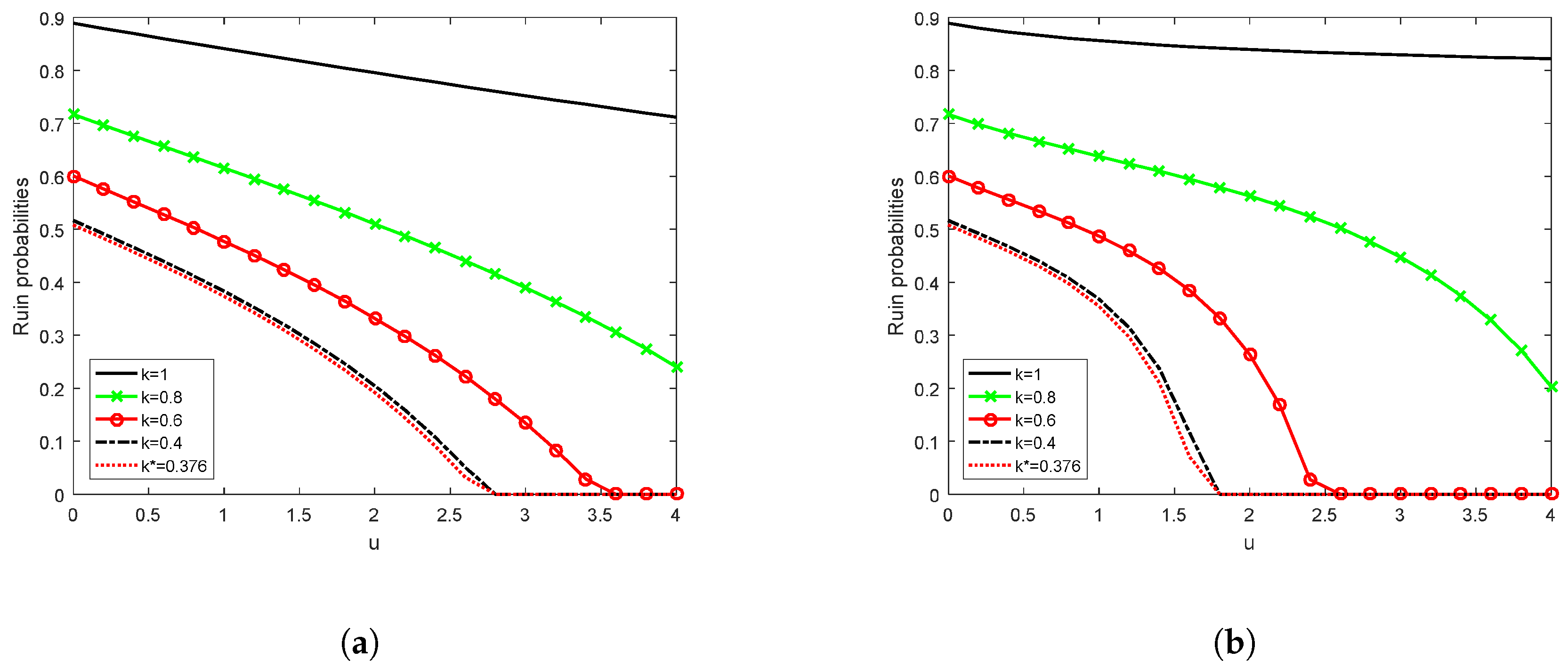
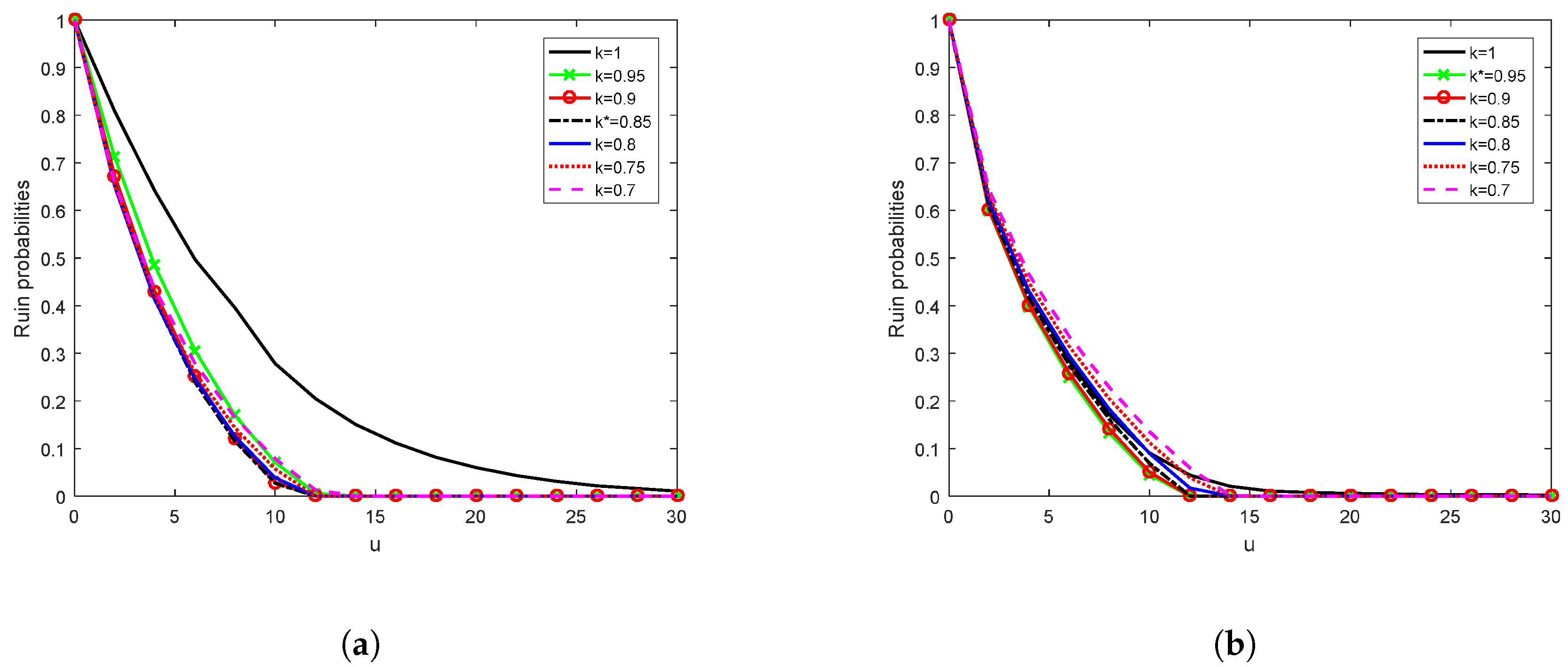
Since the ruin probability is a function of the initial surpus u, we observe from Figure 1a that the ruin probability reduces as the initial surplus increases. We also noted that the higher the cession level $1-k$ for QS reinsurance, the lower the ruin probability. From the results presented in Figure 1, we see that the lowest value of k that satisfies the NPC (4) and at the same time gives the minimal ultimate ruin probability is $0.376$. Thus, the optimal retention for QS reinsurance is $k^{*}=0.376$. This means that the company should cede about $62.4\%$ of its risks to a reinsurer.

Example 2.

Pareto distribution with $\lambda =2,\alpha =3,\kappa =2,\theta =0.8,\eta =0.5$.

The ultimate ruin probabilities for large claims reduce more when QS reinsurance is applied to the portfolio of risks as shown in Figure 1b. As for the small claim case, the optimal QS retention level in the large claim case is $k^{*}=0.376$. Thus, for large claims the insurer must cede about $62.4\%$ of its risks to a reinsurer as well.

4.2. Proportional Reinsurance in the Cramér–Lundberg Model under Interest Force

Here we considered the case when ${\sigma }_1^2={\sigma }_2^2=0$, $r>0$ and $0\le k\le 1$ which lead to the Cramér–Lundberg Model (CLM) compounded by proportional reinsurance and a constant force of interest

$$U_t^k=u+c^{k}t-\sum _{i=1}^{N_t}k{X}_i+r{\int }_0^t{U}_{s}ds.$$

The survival probability satisfies the VIDE

$$(ru+c^k){\varphi }^{\prime }\left(u\right)+\lambda {\int }_0^u[\varphi (u-kx)-\varphi \left(u\right)]dF\left(x\right)=0,$$

(27)

which reduces to a linear VIE of the second kind with kernel and forcing function given in (19).

Example 3.

Exponential distribution with $\lambda =2,\beta =0.5,\mu =1.5,\theta =0.8,\eta =0.5,r=0.05$.

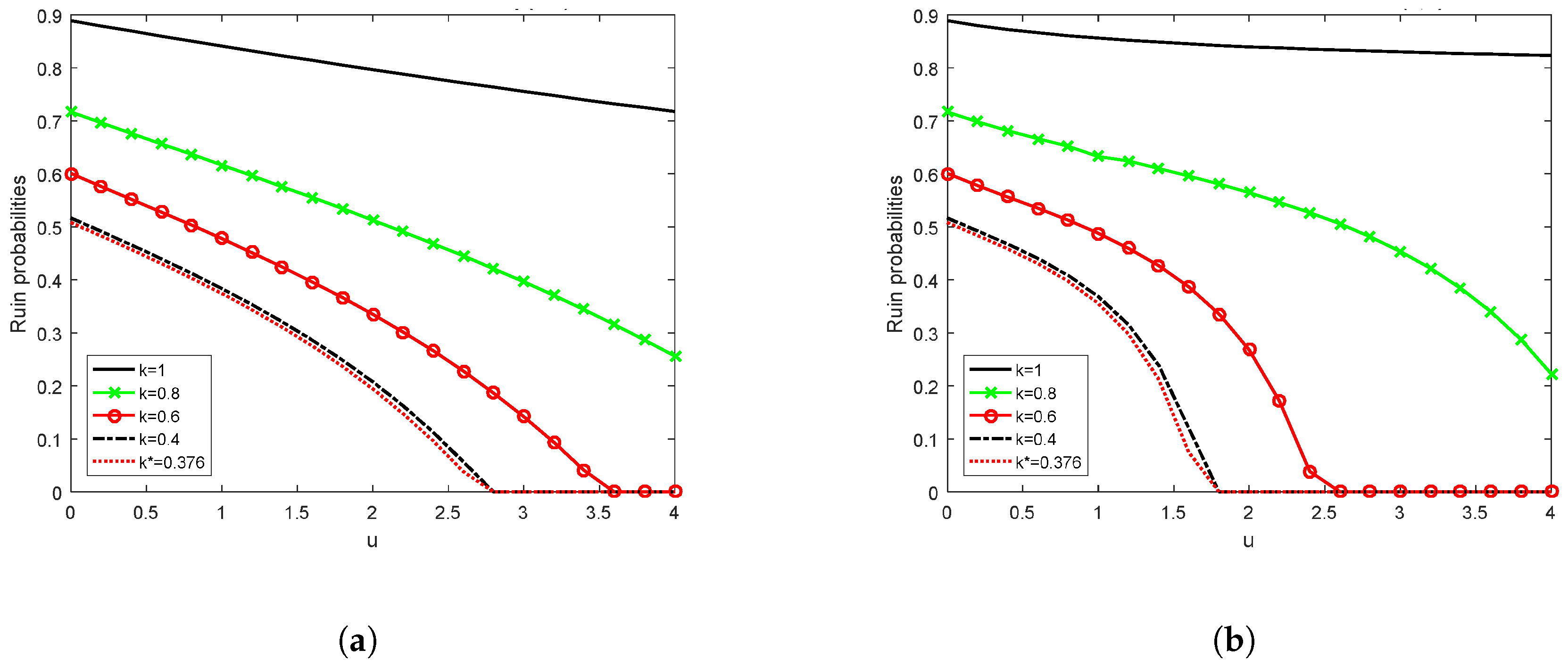
The comments made under Example 1 apply here as well and the optimal QS reinsurance policy in this case is again $k^{*}=0.376$ (see Figure 2a). Though investing part of its surplus in a risk-free asset might provide the insurance company with the flexibility to operate with a lower optimal ruin probability, the company must still reinsure $62.4\%$ of its business as ceding a higher percentage would violate the NPC (Equation (4)).

Example 4.

Pareto distribution with $\lambda =2,\alpha =3,\kappa =2,\mu =1.5,\theta =0.8,\eta =0.5,r=0.05$.

The comments made under Example 2 apply to this case also. Again, the optimal QS reinsurance policy is $k^{*}=0.376$ as shown in Figure 2b. For large claims in the CLM under a constant force of interest, the insurance company must again buy cover for $62.4\%$ of its risks from a reinsurance company.

4.3. Proportional Reinsurance in the Diffusion-Perturbed Model

When ${\sigma }_1^2>0$, ${\sigma }_2^2=r=0$ and $0\le k\le 1$, then we had the diffusion-perturbed model (DPM) compounded by proportional reinsurance

$$U_t^k=u+c^{k}t+k{\sigma }_1{W}_{1,t}-\sum _{i=1}^{N_t}k{X}_i.$$

In this case, the associated VIE has kernel and forcing function given, respectively, by $K(u,x)=\frac{2[c^k-\lambda (u-kx)+\lambda G(u-kx)]}{k^2{\sigma }_1^2}$ and $\alpha \left(u\right)=\frac{u}{k^2}{\varphi }^{\prime }\left(0\right)$. This is simply (20) with ${\sigma }_2^2=r=0$.

Example 5.

Exponential distribution with $\lambda =2,\beta =0.5,\mu =1.5,\theta =0.8,\eta =0.5,r={\sigma }_2=0$, ${\sigma }_1=0.001$.

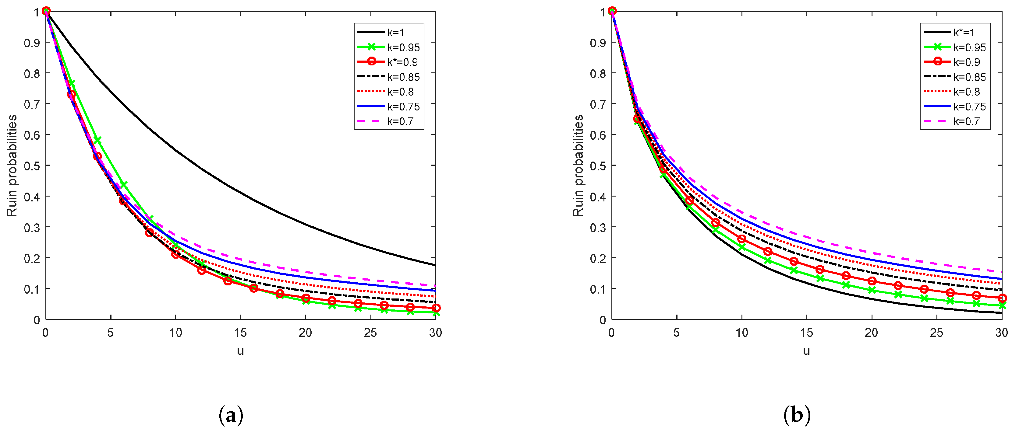
It can be seen from Figure 3a that $k^{*}\approx 0.9$ for $u\in [0,15]$ and $k^{*}=0.95$ for $u\in (15,\infty )$. This means that in the DPM, the insurer should cede $10\%$ of its risks if $u\le 15$ and only $5\%$ if $u>15$. In fact, going by the graph for $k=1$, it is expected that when u is sufficiently large, it is optimal for the company not to reinsure, i.e., $k^{*}=1$.

Example 6.

Pareto distribution with $\lambda =2,\alpha =3,\kappa =2,\theta =0.8,\eta =0.5,r={\sigma }_2=0,{\sigma }_1=0.001$.

For the large claim case in the DPM, the ruin probabilities increase instead of reducing with the application of proportional reinsurance, as can be seen from Figure 3b. We can therefore conclude that it is optimal not to reinsure, i.e., $k^{*}=1$.

4.4. Proportional Reinsurance in the Perturbed Model under Interest Force

This is the case when ${\sigma }_1^2>0$, ${\sigma }_2^2=0$, $r>0$ and $0\le k\le 1$, then we had the DPM compounded by proportional reinsurance and a constant force of interest

$$U_t^k=u+c^{k}t+k{\sigma }_1{W}_{1,t}-\sum _{i=1}^{N_t}k{X}_i+r{\int }_0^t{U}_{s}ds.$$

The corresponding VIE has kernel and forcing function given in (20) with ${\sigma }_2^2=0$.

Example 7.

Exponential distribution with $\lambda =2,\beta =0.5,\mu =1.5,\theta =0.8,\eta =0.5,r=0.05,{\sigma }_1=0.001,{\sigma }_2=0$.

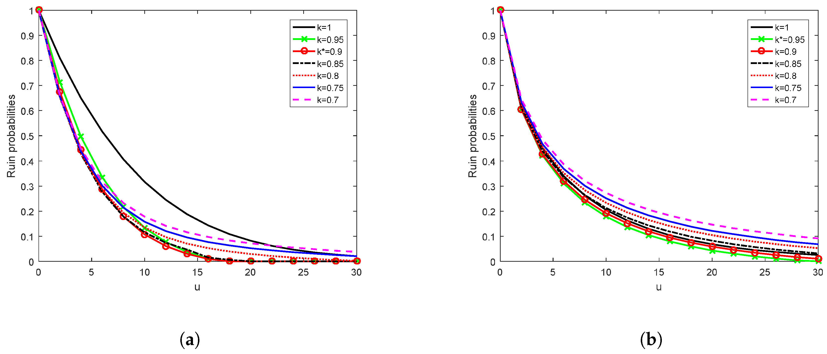
For the DPM under interest force, it is evident from Figure 4a that for exponentially distributed claim sizes the optimal QS reinsurance retention $k^{*}\in (0.85,0.9)$ since the graph for $k=0.85$ is slightly higher for the first time than that for $k=0.9$. Thus, the optimal policy is to reinsure $10\%$ of the risks, i.e., $k^{*}\approx 0.9$.

Example 8.

Pareto distribution with $\lambda =2,\alpha =3,\kappa =2,\theta =0.8,\eta =0.5,r=0.05,{\sigma }_1=0.001,{\sigma }_2=0$.

For the large claim case in the DPM with interest force, Figure 4b shows that the optimal QS retention $k^{*}\in (0.9,0.95)$ since the graph for $k=0.9$ is higher for the first time than that for $k=0.95$. In this case, the company should cede only about $5\%$ of its risks to a reinsurer since $k^{*}\approx 0.95$.

4.5. Proportional Reinsurance with Investments of Black–Scholes Type

When we had stochastic return on investments, the model takes the form

$$U_t^k=u+{\int }_0^t\left(r{U}_s^k+c^k\right)ds+{\int }_0^t\sqrt{{\sigma }_1^2+{\sigma }_2^2{\left(U_s^k\right)}^2}d{W}_s-S_t,U_0^k=u>0.$$

Theorem 2, together with the integrodifferential operator (12), gives the corresponding integrodifferential equation for the survival probability $\varphi \left(u\right)$ as

$$\begin{array}{c}\hfill \frac{1}{2}({\sigma }_2^2{u}^2+k^2{\sigma }_1^2){\varphi }^{{}^{″}}\left(u\right)+(ru+c^k){\varphi }^{{}^{\prime }}\left(u\right)+\lambda {\int }_0^u\varphi (u-kx)dF\left(x\right)-\lambda \varphi \left(u\right)=0\end{array}$$

(28)

for $0\le u\le \infty$, which is a second-order Volterra integrodifferential equation (VIDE). Repeated integration by parts transforms this into a VIE of the second kind with kernel and forcing function as given in (20).

Example 9.

Exponential distribution with $\lambda =2,\beta =0.5,\mu =1.5,\theta =0.8,\eta =0.5,r=0.05,{\sigma }_1={\sigma }_2=0.001$.

This is the small claim case assuming that, in addition to purchasing noncheap proportional reinsurance, the insurance company invests part of its surplus in risk-free and risky assets according to the Black–Scholes options pricing formula. As shown in Figure 5a, the optimal QS retention $k^{*}\in (0.8,0.85)$. From the graph, we see that $k^{*}\approx 0.85$, meaning that the company should reinsure about $15\%$ of its risks.

Example 10.

Pareto distribution with $\lambda =2,\alpha =3,\kappa =2,\theta =0.8,\eta =0.5,r=0.05,{\sigma }_1={\sigma }_2=0.001$.

For the large claim case in the model involving investments of Black–Scholes type, $k^{*}\in (0.9,0.95)$ as shown in Figure 5b. In fact, $k^{*}\approx 0.95$, meaning that the company needs to transfer only $5\%$ of its portfolio of risks to a reinsurer.

4.6. Sensitivity of Ruin Probability to Volatility of Stock Prices

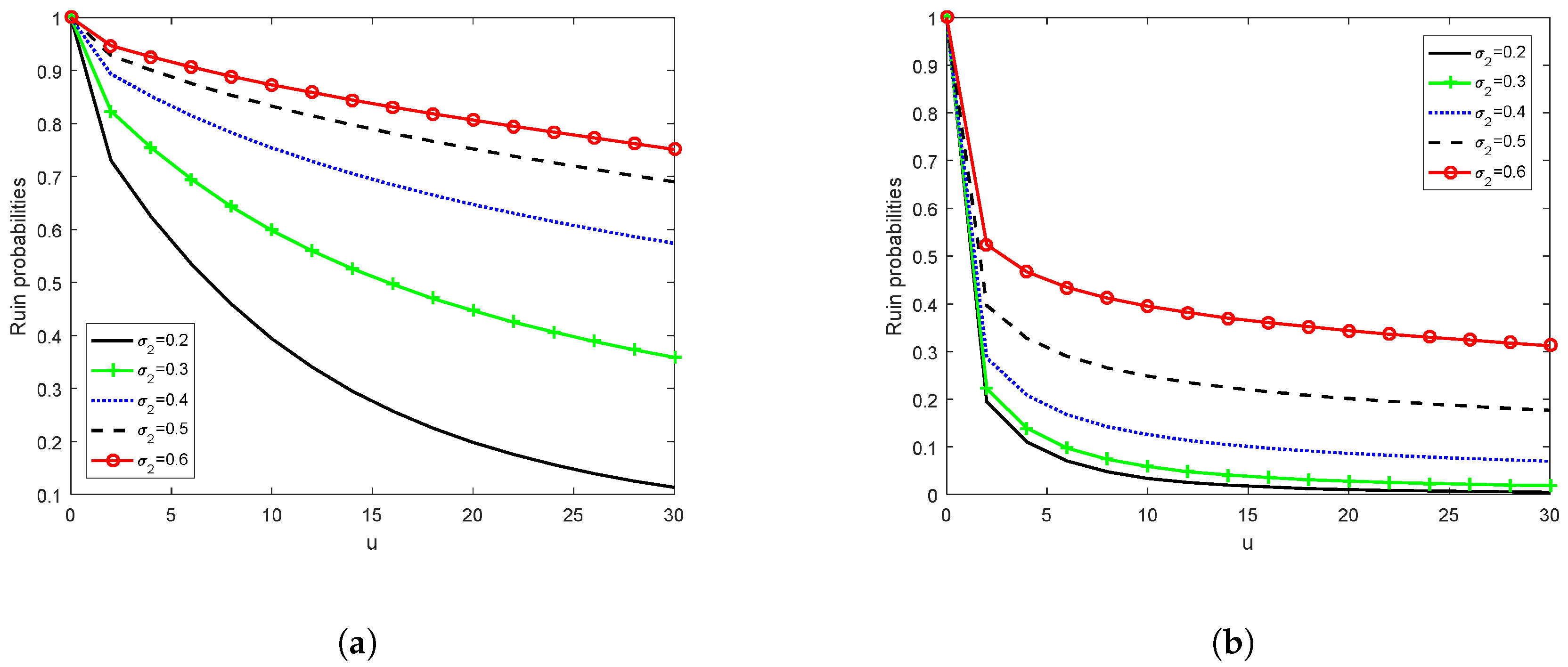
Figure 6 shows the effect of volatility of stock prices on the ultimate ruin probability. Evidently, as stock prices become more volatile (that is, as ${\sigma }_2$ increases), the ruin probability also increases, and vice versa. Volatility is actually a measure of the riskiness of a stock. If the volatility of the stock price increases but the expected rate of return of the stock stays the same, then the insurer will find the reward for accepting the risk unattractive and would rather invest less in stocks and more in bonds. Conversely, a decrease in the volatility of the stock price enables the insurer to receive the same return but with a lower risk. For this reason, the company will find that it makes economic sense to invest in the stock. This applies to both the exponential and Pareto distributions as Figure 6 shows.

However, we also observe from Figure 6 that the ruin probabilities for large claims are much lower than those for small claims.

5. Conclusions

It is evident from the research findings that in the CLM, the ruin probabilities keep reducing as k reduces up to the smallest k that satisfies the NPC, so that the optimal QS retention level for both small and large claim cases in the CLM with and without a constant force of interest is $k^{*}=0.376$. However, for the DPM the ruin probabilities keep reducing up to a given retention level, after which they begin to increase. This is true for both small and large claim cases. This means that the optimal retention level for proportional reinsurance lies somewhere around the point at which the ruin probabilities begin to rise again after consistently falling with a reduction in k. This is in line with our expectation that the ruin probabilities should keep reducing as the quota-share retention level reduces and then start rising again after a certain k, giving an indication of where the optimal retention $k^{*}$ lies. The results from the previous section indicate that proportional reinsurance does have a positive impact on the survival of insurance companies as it minimizes their ultimate ruin probabilities.

Overall, the results for the DPM show that in the small claim case the optimal policy is $k^{*}\ge 0.85$, while in the large claim case it is $k^{*}\ge 0.95$. This means that an insurance company should reinsure up to about $15\%$ of its portfolio in the small claim case and only up to about $5\%$ of its risks in the large claim case. The reason for this difference is that since large claims are also extremal and therefore rare the company can afford to retain more of its large-scale risks.

The results presented in this paper indicate that investment of the surplus plays an important role in the survival of insurance companies as it significantly drives down the ultimate ruin probabilities. Noncheap proportional reinsurance also has an impact on the minimization of the ultimate ruin probabilities of insurance companies, thus enhancing their chances of survival in the market. Possible extensions of this work include the use of other forms of reinsurance arrangements (e.g., surplus, excess-of-loss or stop-loss), introduction of jumps in the investment process and use of other controls such as capital injections and portfolio selection.

References

- Bachelier, L. The theory of speculation. Annales Scientifiques de l’École Normale Supérieure 1900, 17, 21–86. [Google Scholar] [CrossRef]
- Liang, Z.B.; Guo, J.Y. Upper bound for ruin probabilities under optimal investment and proportional reinsurance. Appl. Stoch. Model. Bus. Ind. 2008, 24, 109–128. [Google Scholar] [CrossRef]
- Wang, N. Optimal investment for an insurer with exponential utility preferences. Insur. Math. Econ. 2007, 40, 77–84. [Google Scholar] [CrossRef]
- Liang, Z.B.; Guo, J.Y. Optimal combining quota-share and excess of loss reinsurance to maximize the expected utility. J. Appl. Math. Comput. 2011, 36, 11–25. [Google Scholar] [CrossRef]
- Kasozi, J.; Mahera, C.W.; Mayambala, F. Controlling ultimate ruin probability by quota-share reinsurance arrangements. Int. J. Appl. Math. Stat. 2013, 49, 1–15. [Google Scholar]
- Zhou, J.; Deng, Y.; Huang, Y.; Yang, X. Optimal proportional reinsurance and investment for a constant elasticity of variance model under variance principle. Acta Math. Sci. 2015, 35, 303–312. [Google Scholar] [CrossRef]
- Liu, C.S.; Yang, H. Optimal investment for an insurer to minimize its ruin probability. N. Am. Actuar. J. 2004, 8, 11–31. [Google Scholar] [CrossRef]
- Hipp, C.; Plum, M. Optimal investment for insurers. Insur. Math. Econ. 2000, 27, 215–228. [Google Scholar] [CrossRef] [Green Version]
- Schmidli, H. On minimizing the ruin probability by investment and reinsurance. Ann. Appl. Probab. 2002, 12, 890–907. [Google Scholar] [CrossRef]
- Liang, X.; Young, V.R. Minimizing the probability of ruin: Optimal per-loss reinsurance. Insur. Math. Econ. 2018, 82, 181–190. [Google Scholar] [CrossRef]
- Mossin, J. Aspects of rational insurance purchasing. J. Political Econ. 1968, 76, 553–568. [Google Scholar] [CrossRef]
- Zhu, H.; Huang, Y.; Zhou, J.; Yang, X.; Deng, C. Optimal proportional reinsurance and investment problem with constraints on risk control in a general diffusion financial market. ANZIAM J. 2016, 57, 352–368. [Google Scholar]
- Glineur, F.; Walhin, J.F. de Finetti’s retention problem for proportional reinsurance revisited. Math. Stat. 2006, 3, 451–462. [Google Scholar] [CrossRef]
- Jang, B.-G.; Kim, K.T. Optimal reinsurance and asset allocation under regime switching. J. Bank. Financ. 2015, 56, 37–47. [Google Scholar] [CrossRef]
- Zhang, X.; Liang, Z. Optimal layer reinsurance on the maximization of the adjustment coefficient. Numer. Algebra Control Optim. 2016, 6, 21–34. [Google Scholar] [CrossRef] [Green Version]
- Mikosch, T. Non-Life Insurance Mathematics: An Introduction with Stochastic Processes; Springer: Berlin/Heidelberg, Germany, 2004. [Google Scholar]
- Dam, D.K.; Chung, N.Q. On finite-time ruin probabilities in a risk model under quota share reinsurance. Appl. Math. Sci. 2017, 11, 2609–2629. [Google Scholar] [CrossRef]
- Ladoucette, S.A.; Teugels, J.L. Risk Measures for a Combination of Quota-Share and Drop Down Excess-Of-Loss Rinsurance Treaties. 2004. Available online: http://www.eurandom.nl/ (accessed on 15 December 2018).
- Lampaert, I.; Walhin, J.F. On the optimality of proportional reinsurance. Scand. Actuar. J. 2005, 2005, 225–239. [Google Scholar] [CrossRef] [Green Version]
- Hipp, C. Stochastic control with application in insurance. In Stochastic Methods in Finance; Springer: Berlin/Heidelberg, Germany, 2004; pp. 127–164. [Google Scholar]
- Taylor, G.; Buchanan, R. The Management of Solvency. In Classical Insurance Solvency Theory; Cummins, J.D., Derrig, R.A., Eds.; Kluwer Academic Publishers: Boston, MA, USA, 1988; pp. 49–151. [Google Scholar]
- Dufresne, F.; Gerber, H. Risk theory for the compound Poisson process that is perturbed by diffusion. Insur. Math. Econ. 1991, 10, 51–59. [Google Scholar] [CrossRef]
- Morales, M. On the expected discounted penalty function for a perturbed risk process driven by a subordinator. Insur. Math. Econ. 2007, 40, 293–301. [Google Scholar] [CrossRef]
- Sarkar, J.; Sen, A. Weak convergence approach to compound Poisson risk processes perturbed by diffusion. Insur. Math. Econ. 2005, 36, 421–432. [Google Scholar] [CrossRef]
- Li, D.; Li, D.; Young, V.R. Optimality of excess-loss reinsurance under the mean-variance criterion. Insur. Math. Econ. 2017, 75, 82–89. [Google Scholar] [CrossRef]
- Press, W.H.; Teukolsky, S.A.; Vetterling, W.T.; Flannery, B.P. Numerical Recipes in FORTRAN 77: The Art of Scientific Computing, 2nd ed.; Cambridge University Press: Cambridge, UK, 1992. [Google Scholar]
- Young, A. The application of approximate product-integration to the numerical solution of integral equations. Proc. R. Soc. Lond. Ser. A 1954, 224, 561–573. [Google Scholar]
- Katani, R.; Shahmorad, S. The block-by-block method with Romberg quadrature for the solution of nonlinear Volterra integral equations on large intervals. Ukr. Math. J. 2012, 64, 1050–1063. [Google Scholar] [CrossRef]
- Linz, P. Analytical and Numerical Methods for Volterra Equations; Society for Industrial and Applied Mathematics: Philadelphia, PA, USA, 1985. [Google Scholar]
- Baharum, N.A.; Majid, Z.A.; Senu, N. Solving Volterra integrodifferential equations via diagonally implicit multistep block method. Int. J. Math. Math. Sci. 2018, 2018, 7392452. [Google Scholar] [CrossRef]
- Gatto, R.; Baumgartner, B. Saddlepoint approximations to the probability of ruin in finite time for the compound Poisson risk process perturbed by diffusion. Methodol. Comput. Appl. Probab. 2016, 18, 217–235. [Google Scholar] [CrossRef]
- Gatto, R.; Mosimann, M. Four approaches to compute the probability of ruin in the compound Poisson risk process with diffusion. Math. Comput. Model. 2012, 55, 1169–1185. [Google Scholar] [CrossRef]
- Assari, P. The thin plate spline collocation method for solving integro-differential equations arisen from the charged particle motion in oscillating magnetic fields. Eng. Comput. 2018, 35, 1706–1726. [Google Scholar] [CrossRef]
- Assari, P.; Dehghan, M. A local Galerkin integral equation method for solving integro-differential equations arising in oscillating magnetic fields. Mediterr. J. Math. 2018, 15, 90. [Google Scholar] [CrossRef]
- Cardone, A.; Conte, D.; D’Ambrosio, R.; Paternoster, B. Collocation methods for Volterra integral and integro-differential equations: A review. Axioms 2018, 7, 45. [Google Scholar] [CrossRef]
- Linz, P. A method for solving nonlinear Volterra integral equations of the second kind. Math. Comput. 1969, 23, 595–599. [Google Scholar] [CrossRef]
- Saify, S.A.A. Numerical Methods for a System of Linear Volterra Integral Equations. Master’s Thesis, University of Technology, Baghdad, Iraq, 2005. [Google Scholar]
- Kasozi, J.; Paulsen, J. Flow of dividends under a constant force of interest. Am. J. Appl. Sci. 2005, 2, 1389–1394. [Google Scholar] [CrossRef]
- Paulsen, J.; Kasozi, J.; Steigen, A. A numerical method to find the probability of ultimate ruin in the classical risk model with stochastic return on investments. Insur. Math. Econ. 2005, 36, 399–420. [Google Scholar] [CrossRef]
- Kasozi, J.; Paulsen, J. Numerical Ultimate Ruin Probabilities under Interest Force. J. Math. Stat. 2005, 1, 246–251. [Google Scholar] [CrossRef]
- Paulsen, J. Optimal dividend payouts for diffusions with solvency constraints. Financ. Stoch. 2003, 7, 457–473. [Google Scholar] [CrossRef]
- Paulsen, J.; Gjessing, H.K. Optimal choice of dividend barriers for a risk process with stochastic return on investments. Insur. Math. Econ. 1997, 20, 215–223. [Google Scholar] [CrossRef]
- Paulsen, J. Ruin models with investment income. Probab. Surv. 2008, 5, 416–434. [Google Scholar] [CrossRef]
- Kasumo, C.; Kasozi, J.; Kuznetsov, D. On minimizing the ultimate ruin probability of an insurer by reinsurance. J. Appl. Math. 2018, 2018, 9180780. [Google Scholar] [CrossRef]
- Ma, J.; Bai, L.; Liu, J. Minimizing the probability of ruin under interest force. Appl. Math. Sci. 2008, 17, 843–851. [Google Scholar]
- Schmidli, H. Optimal proportional reinsurance policies in a dynamic setting. Scand. Actuar. J. 2001, 1, 55–68. [Google Scholar] [CrossRef]
- Paulsen, J. Risk theory in a stochastic economic environment. Stoch. Proc. Appl. 1993, 46, 327–361. [Google Scholar] [CrossRef] [Green Version]
- Paulsen, J.; Gjessing, H.K. Ruin Theory with stochastic return on investments. Adv. Appl. Probab. 1997, 29, 965–985. [Google Scholar] [CrossRef]
- Kasumo, C. Minimizing the Probability of Ultimate Ruin by Proportional Reinsurance and Investment. Master’s Thesis, University of Dar es Salaam, Dar es Salaam, Tanzania, 2011. [Google Scholar]
- Schmidli, H. Stochastic Control in Insurance; Springer: London, UK, 2008. [Google Scholar]
- Huang, J.; Tang, Y.; Vázquez, L. Convergence analysis of a block-by-block method for fractional differential equations. Numer. Math. Theor. Methods Appl. 2012, 5, 229–241. [Google Scholar] [CrossRef]
- Kasumo, C.; Kasozi, J.; Kuznetsov, D. Dividend maximization in a diffusion-perturbed classical risk process compounded by proportional and excess-of-loss reinsurance. Int. J. Appl. Math. Stat. 2018, 57, 68–83. [Google Scholar]
- Cheng, G.; Zhao, Y. Optimal risk and dividend strategies with transaction costs and terminal value. Econ. Model. 2016, 54, 522–536. [Google Scholar] [CrossRef]
Figure 1.
Ultimate ruin probabilities for the Cramér–Lundberg Model (CLM) compounded by proportional reinsurance; (a) CLM with quota-share (QS) reinsurance, Exp(0.5) claims; (b) CLM with QS reinsurance, Par(3,2) claims.
Figure 2.
Ultimate ruin probabilities for the CLM compounded by proportional reinsurance and a constant force of interest; (a) CLM with interest force, Exp(0.5) claims; (b) CLM with interest force, Par(3,2) claims.
Figure 3.
Ultimate ruin probabilities for the diffusion-perturbed model (DPM) compounded by proportional reinsurance; (a) DPM with QS reinsurance, Exp(0.5) claims; (b) DPM with QS reinsurance, Par(3,2) claims.
Figure 4.
Ultimate ruin probabilities for the DPM compounded by proportional reinsurance and a constant force of interest; (a) DPM with interest force, Exp(0.5) claims; (b) DPM with interest force, Par(3,2) claims.
Figure 5.
Ultimate ruin probabilities for the DPM compounded by proportional reinsurance and investments of Black–Scholes type; (a) DPM with stochastic interest, Exp(0.5) claims; (b) DPM with stochastic interest, Par(3,2) claims.
Figure 6.
Effects of volatility of stock prices on the ultimate ruin probability in the small and large claim cases; (a) Effect of volatility coefficient on , Exp(0.5) claims; (b) Effect of volatility coefficient on , Par(3,2) claims.
© 2019 by the author. Licensee MDPI, Basel, Switzerland. This article is an open access article distributed under the terms and conditions of the Creative Commons Attribution (CC BY) license (http://creativecommons.org/licenses/by/4.0/).
Share and Cite
MDPI and ACS Style
Kasumo, C. Minimizing an Insurer’s Ultimate Ruin Probability by Reinsurance and Investments. Math. Comput. Appl. 2019, 24, 21. https://doi.org/10.3390/mca24010021
AMA Style
Kasumo C. Minimizing an Insurer’s Ultimate Ruin Probability by Reinsurance and Investments. Mathematical and Computational Applications. 2019; 24(1):21. https://doi.org/10.3390/mca24010021
Chicago/Turabian StyleKasumo, Christian. 2019. "Minimizing an Insurer’s Ultimate Ruin Probability by Reinsurance and Investments" Mathematical and Computational Applications 24, no. 1: 21. https://doi.org/10.3390/mca24010021